1. Introduction
Satellite synthetic aperture radar interferometry (InSAR) is a powerful method for deriving the surface flow pattern and surface elevation of ice sheets and glaciers. Measurements from ascending and descending satellite tracks give two relations between the three components of the surface velocity vector (Reference Joughin, Kwok and FahnestockJoughin and others, 1996). In order to directly measure the full three-dimensional velocity vector, three look directions are required. With the exception of a 6 day period of the RADARSAT Antarctic Mapping Mission1 (Reference Gray, Mattar, Vachon and SteinGray and others, 1998), measurements from three look directions have not been achieved with the satellite systems presently available, which have only provided measurements from two look directions. In order to remedy this shortcoming, an assumption of surface-parallel flow (SPF) has often been used as an approximation to establish a third relationship needed to derive all three components of the velocity vector (Reference Joughin, Kwok and FahnestockJoughin and others, 1998; Reference Mohr, Reeh and MadsenMohr and others, 1998).
Reference Reeh, Madsen and MohrReeh and others (1999a) discussed this assumption, which neglects the influence of local mass balance and a possible contribution to the vertical velocity arising if the glacier is not in steady state. They derived a relationship between the surface velocity components by applying the principle of mass conservation (MC) locally to a vertical column through the glacier. This relationship, valid for both steady-state and non-steady-state conditions, depends on quantities such as ice thickness, the depth distributions of snow/ice density and horizontal velocity, and the local specific mass balance (accumulation or ablation).
In this paper, we derive three-dimensional surface velocities of Storstrømmen, a large outlet glacier from the East Greenland ice sheet located at 77°10′ N, 22°30′ W (see insert in Fig. 1), by combining InSAR measured velocity components from ascending and descending orbits with the MC relationship. We compare the derived velocities to the InSAR velocities previously obtained by Reference Mohr, Reeh and MadsenMohr and others (1998) using the SPF condition and to velocities measured by in situ GPS observations. An analysis of the accuracy of the derived velocities is given by Reference Mohr, Reeh and MadsenMohr and others (2003).

Fig. 1 Map of the Storstrømmen study area. In the light shaded area, ERS-1/-2 InSAR measurements from both ascending and descending orbits are available, supplying two relations between the three surface-velocity components. Arrows marked a and d indicate look direction from ascending and descending orbits, respectively. In the dark shaded area, ice-thickness measurements are also available, permitting set-up of a third relationship between the velocity components. Inside this area, the three velocity components can therefore be derived. The dotted line is the flight track of airborne ice-radar measurements. The large black dots with numbers show the locations of stakes used for in situ GPS velocity measurements.
2. Storstrømmen Glacier
The drainage basin of Storstrømmen extends to Summit, the highest point of the Greenland ice sheet. The area of the drainage basin is approximately 55 000 km2 and the total accumulation in the basin amounts to about 9.8 km3 a−1 (Reference Reeh, Mayer, Miller, Thomsen and WeidickReeh and others 1999b). The extent of the ablation area of Storstrømmen is almost 100 km from south to north. In the east–west direction the width of the ablation area is 20–50 km.
Between 1978 and 1984 the front of Storstrømmen advanced by >10 km. During this surge, the average velocity in the front region of the glacier reached 4 km a−1 as compared to a normal flow rate on the order of 100 ma−1 (Reference Reeh, Bøggild and OerterReeh and others, 1994; Reference Jung-RothenhäuslerJung-Rothenhäusler, 1998). The advance was accompanied by a substantial redistribution of ice along the glacier. In the upper part of the ablation region, surface elevations in 1993 (9 years after the surge) were up to 80 m lower than in 1978. In the lower part of the ablation region, on the other hand, surface elevations in 1993 were up to 80 m higher than in 1978 (Reference Reeh, Bøggild, Jung-Rothenhäusler and OerterReeh and others, 1995; Reference Jung-RothenhäuslerJung-Rothenhäusler, 1998).
At present, Storstrømmen is in a phase of recovery after the surge, and substantial transient ice-thickness and ice-flow changes are occurring (Reference Reeh, Bøggild, Jung-Rothenhäusler and OerterReeh and others, 1995; Reference Jung-RothenhäuslerJung-Rothenhäusler, 1998). Presently, the flow of ice into the glacier complex Storstrømmen–Kofoed Hansen Bræ (the latter is the northeast branch of the glacier system) is effectively blocked by two plugs of nearly stagnant ice (Reference Mohr, Reeh and MadsenMohr and others, 1998). As a consequence, the ice is presently piling up in the region behind the stagnant ice plugs, which, on the other hand, are subject to substantial thinning due to ice ablation. Global positioning system (GPS) measurements in the period 1992–95 show a general, annual decrease of the horizontal surface velocities outside the stagnant ice plugs on the order of 10 m a−2. The GPS measurements also show that summer velocities are larger than the annual means (Reference Mohr, Reeh and MadsenMohr and others, 1998), probably due to meltwater penetrating to the glacier bottom, thereby increasing sliding.
3. Equations for Determining the Ice-velocity Vector
InSAR measurements from ascending and descending orbits provide two relations between the components of the ice-flow velocity vector ![]() :
:
where indices e, n, and u denote east, north and up components, and v
a and v
d denote the components of the velocity vector projected onto the radar line-of-sight directions ![]() and
and ![]() from the ascending and descending orbits, respectively.
from the ascending and descending orbits, respectively.
If a digital elevation model (DEM) of the ice surface is available, each of Equations (1a) and (1b) can be derived from one interferogram, and v a or v d represents the velocity component in the repeat interval (e.g. 1 day for European Remote-sensing Satellite (ERS-1/-2) tandem data). In our Storstrømmen study, a DEM is not used to remove the topography component from the interferometric phase, and Equations (1a) and (1b) are derived by differencing pairs of interferograms with the underlying assumption that the velocity component has the same magnitude in the repeat periods of the two interferograms. In general, glacier flow changes with time, and this is also the case for Storstrømmen. The effect of non-steady-state flow on SAR velocity components derived by differencing pairs of interferograms is discussed by Reference Mohr, Madsen and SteinMohr and Madsen (1999) and, in more detail, by Reference Mohr, Reeh and MadsenMohr and others (2003). They show that, choosing interferograms with the same temporal baseline and spatial baselines of opposite sign, the derived velocity component (ascending or descending) is a weighted average of the velocities corresponding to the acquisition times of the two interferograms, with larger weight to the velocity at the time of the acquisition with the shorter spatial baseline.
Equations (1a) and (1b) provide two equations between the three components of the surface velocity vector. A third equation can be established either on the basis of the kinematic boundary condition at the glacier surface, or by assuming that the horizontal direction of the ice motion is known.
3.1. Known direction of ice motion
If the horizontal direction of the ice motion ![]() is known, a third equation, only involving the horizontal surface velocity
is known, a third equation, only involving the horizontal surface velocity ![]() applies:
applies:
In interior ice-sheet regions, ice flow is approximately in the direction of the maximum surface slope. Hence
where the surface gradient must be derived from an ice-sheet surface smoothed by a low-pass filter that suppresses undulations with wavelengths less than several multiples of the local ice thickness. A low-pass filter with a smoothing distance on the order of 10 times the ice thickness should be applied. Near the ice margin, where bottom sliding may constitute a significant fraction of the motion, Equation (3) may not apply. However, on valley glaciers or ice margins, the horizontal flow direction can often be determined approximately from surface flow features (e.g. derived from satellite imagery) or from the direction of confining valley walls. In this case, Equation (2) can be used directly as the third equation.
3.2. Surface boundary condition
Alternatively, a third equation can be established by using the kinematic boundary condition at the glacier surface relating the instantaneous rate of change of surface elevation ∂S/∂t to the ice-particle velocity vector ![]() and the instantaneous specific mass balance b
S(t) (positive as accumulation, negative as ablation measured in metres snow/ice per unit time) (Reference Reeh, Madsen and MohrReeh and others, 1999a):
and the instantaneous specific mass balance b
S(t) (positive as accumulation, negative as ablation measured in metres snow/ice per unit time) (Reference Reeh, Madsen and MohrReeh and others, 1999a):
where ![]() is the surface normal vector and t is time.
is the surface normal vector and t is time.
In order to apply this equation to derive the velocity components, the lefthand side must be known from either direct measurement or calculation. In general, all three members of Equation (1c) change with time. Ideally, the lefthand side of Equation (1c) should therefore be determined as a mean value over the acquisition periods of the interferograms used for deriving Equations (1a) and (1b). In the real world, measurements of ∂S/∂t and b S(t) are based on observations over a certain time interval Δt = t 2 − t 1 that, in general, is considerably longer than the relevant InSAR acquisition periods, and often does not even encompass those periods. Application of Equation (1c) therefore implies assumptions that seldom are exactly fulfilled.
To account for the fact that, in practice, the lefthand side of Equation (1c) is based on measurements over a certain period of time, we integrate Equation (1c) with respect to time:

from which
where underlined quantities represent average values over the time period Δt that usually is on the order of magnitude of 1 year. Here we shall assume that Δt is 1 year.
Many glaciers and ice-sheet margins display significant seasonal variations of surface velocity, with generally higher velocities in the summer than in the winter. As a first approximation, we shall assume that only the magnitude of the velocity vector varies seasonally but that the flow pattern (the particle paths) remains unchanged, i.e. ![]() , where f(t) is a seasonal variable subject to the condition
, where f(t) is a seasonal variable subject to the condition ![]() . Assuming that seasonal variations of n
s can be neglected, we then obtain
. Assuming that seasonal variations of n
s can be neglected, we then obtain
For a glacier in steady state we have by definition (S 2 − S 1)/Δt = 0, and the equation above is therefore reduced to
where b s denotes the mean annual specific mass balance measure in metres snow/ice per year.
Equation (1d) is often further simplified by assuming SPF:
Reference Reeh, Madsen and MohrReeh and others (1999a) discussed the application of Equations (1d) and (1e) and concluded that it is not always satisfactory to apply these equations. They suggested using a relation derived from the MC principle valid for both steady-state and non-steady-state conditions. In the ablation zone of a grounded glacier with negligible bottom melting, this equation reads
where h is ice thickness and ![]() is a velocity profile factor. u denotes the magnitude of the two-dimensional, horizontal velocity vector
is a velocity profile factor. u denotes the magnitude of the two-dimensional, horizontal velocity vector ![]() . Subscript S refers to the glacier surface, and underline denotes column mean value.
. Subscript S refers to the glacier surface, and underline denotes column mean value. ![]() is the two-dimensional horizontal gradient operator. In a Cartesian coordinate system (x, y) we have
is the two-dimensional horizontal gradient operator. In a Cartesian coordinate system (x, y) we have ![]() .
.
Reference Reeh, Madsen and MohrReeh and others (1999a) made the assumption that the velocity profile factor was only weakly dependent on x and y, and consequently F was moved outside the gradient operator. Certainly, in our application of Equation (1f) to the Storstrømmen example, we use a constant value of F = 0.95. However, in the error assessment (Reference Mohr, Reeh and MadsenMohr and others, 2003) spatial variation of F is considered. To maintain consistency, we therefore keep F inside the gradient operator in Equation (1f).
There are several reasons to use Equation (1f) to derive the velocity field of Storstrømmen instead of one of the simpler Equations (1d), (2) or (3). Storstrømmen is presently in a post-surge state (non-steady-state), making Equation (1d) a problematic choice. Moreover, in extended areas of Storstrømmen, the flow direction deviates significantly from the local surface gradient (Reference Mohr, Reeh and MadsenMohr and others,1998), impeding estimation of reliable flow directions. Finally, a prerequisite for applying Equation (1f) is fulfilled for Storstrømmen as the ice-thickness distribution is known from airborne ice-sounding radar measurements.
In component form, Equations (1a), (1b) and (1f) may be written:
ψ and θ are azimuth and angle of incidence (relative to a level surface) of the radar look direction. ψ is measured relative to east in the counterclockwise direction. Subscripts a and d refer to ascending and descending orbit tracks, respectively. Note that for a right-looking radar, ψ is equivalent to the ground-track angle measured relative to north in a clockwise direction.
The SAR processing algorithm (Mohr and others,1997) provides the coefficients to v e, v n and v u on the lefthand sides of Equations (4a), (4b) and (4f) in a regular geographical coordinate grid. If the glacier thickness h and the velocity-profile factor F (see below) are also known at the grid-points, the three components of the velocity vector can be determined unambiguously by an iterative procedure.
It is worth noticing that, for points with θ a ≈ θ d , we have ψ d ≈ 180 − ψ a. In this case, the east component of the velocity v e can be found directly from the line-of-sight velocities v a and v d (Reference Mohr, Madsen and SteinMohr and Madsen, 1999; Reference Mohr, Reeh and MadsenMohr and others, 2003). For our Storstrømmen example, the symmetry condition is fulfilled sufficiently well to allow such a direct calculation of v e. However, in order to determine the north and up components of the velocity, the third equation is required.
4. Method of Solution
The equation system (4a, b, f) is solved iteratively using the following procedure which proved to converge rapidly: Initially, the righthand side of Equation (4f) is put equal to zero, and the system of three linear equations is solved at each gridpoint. This corresponds to the hitherto applied procedure of assuming SPF. Next, the horizontal ice-flux components are calculated at each gridpoint as Fhv e and Fhv n, respectively, and the flux divergence is calculated by summing the relevant derivatives. Using this flux-divergence term as the righthand side of Equation (4f), an improved solution to the system of equations can be found. Due to the magnification of errors, generally related to the process of forming derivatives numerically, the derived flux-divergence field displays large fluctuations on length scales comparable to the grid spacing of 500 m by 500 m. Such high-frequency oscillations of the flux-divergence field are not physically acceptable. Moreover, application of the raw flux-divergence field will cause the iteration process to diverge. For these reasons, the flux-divergence field is smoothed by low-pass filtering (using a simple, 21 times 21 points box filter) before being used on the righthand side of Equation (4f) for the next step of the iteration procedure. With this smoothing, only three to four iteration cycles are needed in order to obtain a stable velocity solution. Reference Kamb and EchelmeyerKamb and Echelmeyer (1986) show that a triangular filter rather than a box (rectangular) filter is preferable when dealing with the influence on glacier flow of longitudinal stress variations caused by local slope and ice-thickness changes. This may also be true for our case of smoothing the flux-divergence field. However, replacing the box filter with a triangular filter does not significantly change the derived velocities. Moreover, the error analysis presented by Reference Mohr, Reeh and MadsenMohr and others (2003) is simplified by the use of a rectangular filter. An analysis of the criterion for stability of the solution is beyond the scope of the present paper. However, it can be noted that, even after 200 iteration cycles, no sign of instability was detected.
5. Measurements
The measurements on Storstrømmen used in this study comprise global positioning system (GPS) positions of stakes drilled into the glacier, elevation and line-of-sight velocity measurements from interferometric radar, and ice-thickness data from low-frequency airborne ice-sounding radar. The areas covered by the different measurements are shown on the map in Figure 1.
5.1. GPS stake position measurements
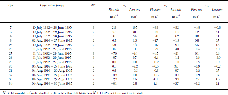
Fieldwork on Storstrømmen was carried out during the six seasons 1989–95 by the Alfred-Wegener-Institut für Polar und Meeresforschung (AWI), Bremerhaven, Germany, and the Danish Polar Center, Copenhagen, Denmark (Reference Oerter, Bøggild, Jung-Rothenhäusler and ReehOerter and others, 1995; Reference Reeh, Bøggild, Jung-Rothenhäusler and OerterReeh and others, 1995). Positions of 23 stakes (14 inside the study area) drilled into the ice surface were repeatedly measured with Transit satellite Doppler surveying (1989–90) and differential GPS (1992–95). Velocities derived from these measurements were previously used to validate the horizontal InSAR velocities determined by Reference Mohr, Reeh and MadsenMohr and others (1998) using the assumption of surface-parallel flow. In this study, we only use velocities derived from the more accurate GPS measurements (see Table 1). A comparison of the columns in the table showing first and last observations suggests a long-term decreasing trend of the horizontal velocities of points outside the stagnant region of the glacier. This trend is confirmed by the results of the Doppler survey.
Table 1 In situ GPS velocity measurements on Storstrømmen

5.2. Extrapolation of GPS data
The GPS data have therefore been re-analyzed in order to account for temporal long-term trends. This is important because the SAR images were acquired in winter 1995/96 (see section 5.3), i.e. half a year after the last GPS observations.
The temporal variation of the GPS velocities is illustrated in Figure 2, using the motion of pole 7 as an example (for location, see Fig. 1). The step-curves in Figure 2 show the variation of the west–east, south–north and vertical velocity components of pole 7. The velocity components (mean values over the observation periods) are plotted vs the distance accomplished by the pole from August 1989 to June 1995. Observation-day numbers, counted from 1 January 1989, are written along the step-curves, showing that all velocities are averaged over an interval of at least 1 year. The velocity components display a clear trend as well as a fluctuation around the trend lines (dashed lines in Fig. 2). Observations from two summer periods (not shown in Fig. 2), one at the beginning and one at the end of the 5 year observation period, gave velocities that are 30–40% higher than the mean velocities in the adjacent intervals, probably because of meltwater penetrating to the glacier bottom, thereby enhancing sliding. We therefore conclude that, quite likely, the fluctuations of the mean velocities around the trend lines are caused by seasonal velocity variations, as the observed mean velocities are composed of different fractions of summer and winter velocities.

Fig. 2 Variation of the velocity components of pole 7 on Storstrømmen (for location see Fig. 1). The step-curves show mean values over the intervals between Transit Doppler and GPS observations. Observation-day numbers counted from 1 January 1989 are written along the step-curves. Heavy curves labelled “mass conservation” and light curves labelled “surface-parallel-flow” show the spatial variation of the velocity components along the path followed by the pole during the observation period. The curves represent spatial velocity distributions at the time of the InSAR measurement, i.e. 1 February 1996, corresponding to day number 2586 since 1 January 1989. The MC curves are derived from the InSAR velocity maps shown in Figure 4a–c. The SPF curves are derived from similar maps of SPF velocities. Dashed lines are least-squares linear fits to the GPS velocity measurements between day 1287 and day 2370 used to extrapolate the GPS velocities to the estimated position of the pole (distance = 1565 m) on 1 February 1996 (day 2586).
As discussed by Reference Mohr, Reeh and MadsenMohr and others (1998, Reference Mohr, Reeh and Madsen2003), it is reasonable to assume that during winter (September–May), when there is no melting at the surface, the only velocity change is due to the decreasing trend associated with the post-surge, long-term adjustment of ice dynamics. In the non-stagnant regions of the glacier, the corresponding decrease of velocity during the InSAR observation period is 2–3 m a−1. For the validation of the InSAR-derived velocities, we need GPS velocities of the poles on 1 February 1996, the “date”of the InSAR measurement (see section 5.3). These velocities are determined by linear extrapolation if three or more GPS observations are available, or by averaging two observations. If linear extrapolation is used, the correspondig error limits (standard deviation) are calculated as ![]() , where σ
m and σ
b are standard deviations of the mean and slope of the regression line, and t
E and t
m are the time of extrapolation (1 February 1996, i.e. day 2856) and the mean time of the observation period, respectively. In the case of averaging, we use σ
E = σ
m.
, where σ
m and σ
b are standard deviations of the mean and slope of the regression line, and t
E and t
m are the time of extrapolation (1 February 1996, i.e. day 2856) and the mean time of the observation period, respectively. In the case of averaging, we use σ
E = σ
m.
5.3. Interferometric satellite SAR measurement
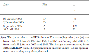
The interferometric SAR measurements of Storstrømmen are based on the ERS-1/-2 tandem data summarized in Table 2. A double-differencing technique is applied, and elevations as well as line-of-sight displacement are derived for both ascending- and descending-orbit data. The elevations used for calculation of surface slopes are based on ascending-orbit data only, due to the superior spatial baseline conditions as compared to the dataset from the descending orbits (see Table 2). The elevations are expected to have an overall accuracy on the order of 10 m (Reference Mohr, Reeh and MadsenMohr and others, 2003).
Table 2 Characteristics of ERS-1/-2 tandem data

A detailed description of the InSAR data and the data processing is given by Reference Mohr, Reeh and MadsenMohr and others (1998) and Mohr and others (1997), respectively. An analysis of the accuracy of the derived velocity solution is presented by Reference Mohr, Reeh and MadsenMohr and others (2003). The error analysis deals with interferometric path-length distortions originating from the atmosphere and an uneven dry snow cover; with baseline calibration errors; with errors due to non-stationary flow; and with errors caused by errors of surface slope, ice thickness and velocity-profile factor F. The major error source for the east component of velocity is shown to be the atmospheric disturbances including the indirect effect of spatially varying baseline errors. For the north and up velocity components that cannot be derived from the interferometric measurements alone, errors of surface slope, ice thickness and the F factor also contribute significantly. It is not possible to provide a single number for the accuracy of the velocities, as the error depends on quantities such as distance from ground-control points and ice thickness. Maps showing the estimated distribution of the errors of the velocity components are provided by Reference Mohr, Reeh and MadsenMohr and others (2003).
As mentioned previously, the line-of-sight velocities derived from descending- and ascending-orbit data represent velocities on different days, i.e. approximately 2 December 1995 and 10 April 1996, respectively. During the intervening period, the velocities in the non-stagnant region of Storstrømmen changed by 2–3 m a−1 (see section 5.2). The error analysis shows that, if we choose 1 February 1996 (the mid-point of the above interval) as the “date” of the InSAR velocity observation, then the temporal velocity change will only result in small errors of the derived InSAR velocities as compared to the atmosphere and baseline errors.
5.4. Airborne ice-thickness radar measurement
The ice thickness was measured at an airborne ice-sounding radar survey of Storstrømmen in August 1993. The measurements were performed using the Technical University of Denmark 60 MHz ice radar (Reference Christensen, Gundestrup, Nilsson and GudmandsenChristensen and others, 1970, Reference Christensen, Reeh, Forsberg, Jörgensen, Skou and Woelders2000) flown on a Greenland Air Twin Otter aircraft positioned by means of differential GPS measurements. Altogether 560 km of surface-elevation and ice-thickness profiles were obtained from the ablation zone of Storstrømmen (see map in Fig. 1). Combining these data with a DEM of the ice-free land surrounding the glacier, a digital grid model of the ice-thickness distribution of Storstrømmen was established. A contoured version of this model is shown in Figure 3.

Fig. 3 Ice-thickness distribution of Storstrømmen derived from airborne ice-sounding radar measurements in August 1993 along the flight track shown as a heavy black line.
Ice-thickness errors include radar noise, smoothing errors, bias due to the radar detecting the echo from the closest (not the nadir) point of the bottom, and grid interpolation errors. For details, the reader is referred to Reference Mohr, Reeh and MadsenMohr and others (2003).
5.5. The velocity-profile factor F
Observations and ice-sheet dynamic model studies suggest values of F between 0.9 and 1 (Reference Reeh and GundestrupReeh and Gundestrup, 1985; Reference Thomas, Csathó, Gogineni, Jezek and KuivinenThomas and others, 1998). Two different processes may cause variations of F. The observed increase of the ratio of summer velocity to mean annual velocity along Storstrømmen indicates that basal sliding constitutes an increasing fraction of the forward motion of the glacier when the glacier terminus is approached. During the summer months, the ratio between sliding velocity and mean column velocity, and consequently the F factor, will therefore increase along the glacier. A variation from F = 0.9 (no bottom sliding) to F = 1.0 (fully developed bottom sliding) can be expected. The InSAR velocities are measured in the winter, when observations indicate that basal sliding is less developed. Nevertheless, for the assessment of the flux-divergence error term, we use a constant F = 0.95 and assume a bias of ±0.05 (see Reference Mohr, Reeh and MadsenMohr and others, 2003).
Flow over basal irregularities also causes variation of the F factor, from large values over basal highs to smaller values over basal lows. As explained by Reference Mohr, Reeh and MadsenMohr and others (2003), such F variations reduce the contribution to the grid-interpolation error of the flux-divergence term from unknown ice-thickness variations.
6. Results
The velocity components derived by using the MC condition are shown in Figure 4a–c. Deviations between these velocity components and the corresponding velocity components derived with the SPF assumption are shown on the maps in Figure 4d–f. Application of the MC condition implies significant changes of the vertical velocity component of up to 5 m a−1 or more. The south–north velocity component is changed by up to 30 m a−1 (20%), whereas the west–east component is essentially unchanged. As mentioned previously, this is in accordance with the finding by Reference Mohr, Madsen and SteinMohr and Madsen (1999) that only the north–south component of the horizontal flow vector derived from ascending- and descending-orbit data is influenced by terrain slope and submergence/emergence velocities.

Fig. 4 (a–c) Surface velocity (m a−1) of Storstrømmen derived from InSAR measurements by using the MC principle. (d–f) Difference (m a−1) between MC velocities and SPF velocities. (a, d) West–east velocity; (b, e) south–north velocity; (c, f) up velocity.
The glaciological implications of the derived velocity fields are discussed elsewhere (Reference ReehReeh and others, 2002). Here we shall only briefly discuss the “difference” map for the vertical velocity component shown in Figure 4f. This difference, representing the horizontal flux-divergence term, is identical to the so-called emergence/submergence velocity (Reference PatersonPaterson, 1994, p. 258). It measures the local upward or downward flow of ice relative to the glacier surface. The large positive emergence velocities displayed in the upper, central part of the map are not compensated by ablation, which in this area is on the order of magnitude of 1 m a−1 of ice (Reference Oerter, Bøggild, Jung-Rothenhäusler and ReehOerter and others, 1995). Consequently, the glacier is thickening in this region at a rate of several metres per year. In contrast, the southern and northeastern parts of the glacier display negative emergence velocities. There, an annual ablation rate in the range 1.5–2 m enhances glacier thinning. This pattern of thickness change, tending to regenerate the glacier surface elevations that occurred prior to the surge, is typical for a glacier in its post-surge stage.
6.1. Comparison with GPS observations
The trends of the velocity components illustrated for pole 7 by the dashed lines in Figure 2 may result from two different processes: they may be due either to “long-term” temporal velocity variations or to movement of the pole through a spatially varying velocity field. How much each of these processes contributes to the trends can be studied by comparing the observed GPS velocity variations with the InSAR-derived velocity distributions along the path followed by the pole during the GPS observation period. These distributions represent the spatial variations of the velocity components at the time of the InSAR measurement (1 February 1996). For each velocity component, two InSAR curves are shown in Figure 2: one is derived from the MC maps in Figure 4a–c, the other from similar SPF maps (not shown in Fig. 4). The differences between the GPS and MC curves represent the temporal change of the velocity components from the time of the GPS velocity observation to 1 February 1996. If there were no seasonal variations of the velocity, the values of the velocity components determined by extrapolation to the estimated position of the pole on 1 February 1996 (day number 2586 since 1 January 1989) should therefore fall on the MC curves. The deviations are due to inaccuracies of InSAR as well as GPS-derived velocities, but probably also to using linear trend lines for extrapolating the GPS velocities. However, the limited number of GPS observations does not justify non-linear fitting and extrapolation. It should also be noticed that the extrapolated GPS velocities are determined by using mean values that include the motion in the summer period, with increased velocities as compared to the winter velocities measured with the interferometric radar.
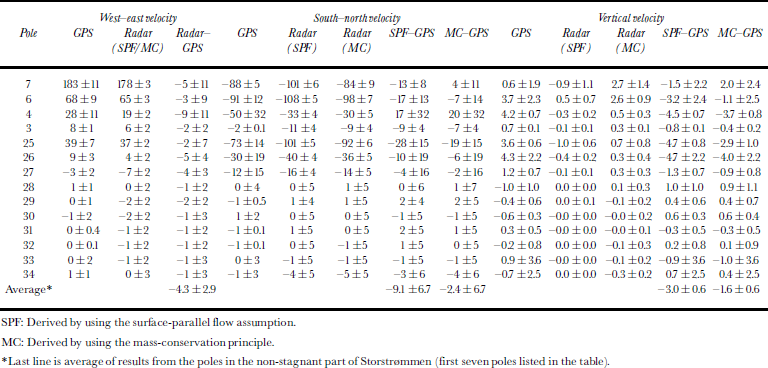
Figure 4 shows that the extrapolated velocities are in better agreement with the MC velocities than with the SPF velocities. This is confirmed by Table 3 in which extrapolated GPS velocities of all poles within the study area are compared with both SPF and MC InSAR-derived velocities. Standard errors of the GPS velocities are determined as described in section 5.2. The standard errors of the InSAR-derived velocities are derived from the error maps presented by Reference Mohr, Reeh and MadsenMohr and others (2003).
Table 3 Comparison of extrapolated GPS velocities with radar velocity measurements on Storstrømmen (units are m a−1)

As mentioned earlier, the west–east components of InSAR-derived velocities are not influenced by the vertical flow, and thus the MC and SPF solutions are expected to be the same, as in fact shown by our calculations. Consequently, only one set of west–east radar velocities is shown in Table 3. The uncertainty of the MC-derived south–north and up components is larger than that of the SPF-derived components, because the uncertainty of the former also includes errors from the flux-divergence term. However, the south–north and up MC velocities are in better agreement with the GPS velocities than are the SPF velocities, as reflected in the significantly smaller radar–GPS differences obtained by using the MC velocities. For the poles in the non-stagnant part of Storstrømmen (the first seven poles listed in Table 3), the west–east velocity differences have a mean value of −4.3 m a−1 and a rms value of 2.8 m a−1. The south–north SPF velocity differences have a mean of −9.1 m a−1 and a rms value of 15.7 m a−1, whereas the corresponding values for the MC case are −2.4 and 11.4 m a−1, respectively. The up SPF velocity differences have a mean value of −3.0 m a−1 and a rms value of 3.4 m a−1, whereas the corresponding values for the MC case are −1.6 and 2.5 m a−1, respectively.
The south–north and up MC–velocity differences still have negative biases, as do the west–east velocity differences. Most likely the biases are due to interpolating linearly the GPS velocity data to the “date” of the InSAR velocity measurement. A small non-linear component of the decreasing velocity trend would explain the bias.
7. Conclusions
We have demonstrated that the three-dimensional glacier surface velocity, including the vertical component, can be derived by combining InSAR measurements from ascending and descending satellite tracks with ice-thickness measurements. We have shown that, at present, non-steady-state vertical velocities of up to 5 m a−1 exceed the vertical SPF component over a large part of the ablation area of Storstrømmen. Furthermore, our study shows that neglecting a vertical velocity component of this magnitude may result in substantial errors also on the InSAR-derived horizontal velocities. In south Greenland, and in many other glacierized areas, the vertical velocity component required to balance the annual ablation rate is 5–10 m a−1 or even more. In such cases, it is not advisable to use the SPF assumption when deriving glacier velocities from InSAR measurements, even if the glacier is in steady state. It is possible to account for the vertical ice motion relative to the surface (the emergence/submergence velocity) in different ways. If steady state can be assumed, the emergence/submergence velocity is equal to the local annual specific mass balance b S. If b S is measured, a velocity solution can be derived by using Equations (1a), (1b) and (1d). Otherwise, our approach using the MC condition is recommended. This approach, however, requires detailed measurement of the ice-thickness distribution. In the accumulation zone, the specific mass balance and the depth–density profile must also be known (see Reference Reeh, Madsen and MohrReeh and others, 1999a).
A different approach would be to combine InSAR measurements from ascending and descending orbits with knowledge of the horizontal flow direction of the glacier (e.g. by assuming flow in the direction of the maximum surface slope). This approach can certainly provide three-dimensional glacier surface velocities, but its accuracy remains to be demonstrated.
If three look directions should become available with future SAR systems, the three velocity components can be directly determined from the InSAR measurement. If the ice-thickness distribution is also measured, the equation derived from the MC principle can then be used, for example, to constrain the depth variation of the horizontal ice velocity.
Acknowledgements
F. Jung-Rothenhäusler of the AWI participated in the GPS observation programme on Storstrømmen. W. Starzer of the Geological Survey of Denmark and Greenland helped with the digital ice-thickness model of Storstrømmen. This research was supported by the Commission of the European Communities under contracts EPOC-CT90-0015 and EV5V-CT91-0051, by the European Space Agency AO-2 programme and by the Commission for Scientific Research in Greenland. Constructive criticism by H. Rott (Scientific Editor) and two unknown reviewers resulted in substantial improvements to the paper.