


1. INTRODUCTION
Debris-covered glaciers have been a focus of interest in recent years as the scientific community seeks to gain a better physical understanding of glaciers and climate change in High Mountain Asia (Benn and others, Reference Benn2012; Bolch and others, Reference Bolch2012). Studies have shown that supraglacial ponds and ice cliffs play a key role in the ablation of such glaciers (Benn and others, Reference Benn2012; Immerzeel and others, Reference Immerzeel2014a; Pellicciotti and others, Reference Pellicciotti2015; Steiner and others, Reference Steiner2015; Miles and others, Reference Miles2016; Buri and others, Reference Buri, Pellicciotti, Steiner, Evan and Immerzeel2016). They have also demonstrated that the supraglacial ponded area changes from year to year (Gardelle and others, Reference Gardelle, Arnaud and Berthier2011; Liu and others, Reference Liu, Mayer and Liu2015), which may be related to glacier downwasting in response to climate (Sakai and Fujita, Reference Sakai and Fujita2010; Benn and others, Reference Benn2012). Changes in pond cover on the multiannual (Liu and others, Reference Liu, Mayer and Liu2015) and decadal (Gardelle and others, Reference Gardelle, Arnaud and Berthier2011) timescales are a key point of interest, as a potential indicator and feedback for glacier response to climate warming (Benn and others, Reference Benn2012) and as an early warning for the formation of proglacial lakes (e.g. Bolch and others, Reference Bolch, Buchroithner, Peters, Baessler and Bajracharya2008; Benn and others, Reference Benn2012).
Understanding of key processes leading to the formation of supraglacial ponds has advanced conceptually to include conduit-collapse formation (Kirkbride, Reference Kirkbride1993; Sakai and others, Reference Sakai, Takeuchi, Fujita and Nakawo2000), subaqueous and waterline melting (Sakai and others, Reference Sakai, Takeuchi, Fujita and Nakawo2000; Röhl, Reference Röhl2006; Miles and others, Reference Miles2016), calving (Benn and others, Reference Benn, Wiseman and Hands2001; Sakai and others, Reference Sakai, Nishimura, Kadota and Takeuchi2009) and englacial filling and drainage (Gulley and Benn, Reference Gulley and Benn2007). The behaviour of ponds across an entire glacier, however, has received little attention, as most process-oriented field observations have been made of individual features (Benn and others, Reference Benn, Wiseman and Hands2001; Röhl, Reference Röhl2008; Xin and others, Reference Xin, Shiyin, Han, Jian and Qiao2011), while whole-glacier studies have often used a single satellite scene and are limited temporally (e.g. Panday and others, Reference Panday, Bulley, Haritashya, Ghimire, Thakur, Singh, Ramanathan, Prasad and Gossel2012; Salerno and others, Reference Salerno2012). Controls on the spatial distribution of ponds have been suggested, including surface gradient, mass balance, cumulative surface lowering and surface velocity (Reynolds, Reference Reynolds2000; Quincey and others, Reference Quincey2007; Sakai and Fujita, Reference Sakai and Fujita2010; Salerno and others, Reference Salerno2012; Sakai, Reference Sakai2012).
Several studies have used satellite data to determine variability of pond distributions across several years or decades (Röhl, Reference Röhl2008; Gardelle and others, Reference Gardelle, Arnaud and Berthier2011; Liu and others, Reference Liu, Mayer and Liu2015; Thompson and others, Reference Thompson, Benn, Mertes and Luckman2016; Watson and others, Reference Watson, Quincey, Carrivick and Smith2016). However, no attempt has been made to document the seasonal variability of ponds, even though individual ponds are known to fill and drain periodically based on field observations (Benn and others, Reference Benn, Wiseman and Hands2001; Immerzeel and others, Reference Immerzeel2014a; Liu and others, Reference Liu, Mayer and Liu2015) and although observations suggest increased pond cover leading into the monsoon (Watson and others, Reference Watson, Quincey, Carrivick and Smith2016). Furthermore, satellite observations of supraglacial ponds are severely limited by seasonal cloud cover and snowcover. Consequently, previous studies of changes in pond cover over annual to decadal timescales miss the seasonal variability and may be biased in their assessment of change.
Pond filling and drainage are linked to the supply and timing of rain and meltwater from snow or glacial sources (Benn and others, Reference Benn, Wiseman and Hands2001; Liu and others, Reference Liu, Mayer and Liu2015), the supraglacial routing of that water and the opening and closure of englacial conduits (Gulley and Benn, Reference Gulley and Benn2007). In many respects, therefore, the controls on the spatial and temporal distribution of ponds on debris-covered glaciers are similar to those of lakes on clean-ice glaciers (Boon and Sharp, Reference Boon and Sharp2003). Understanding the controls and timing of pond filling and draining is important from a mass-balance perspective. Pond-associated melt enhancement, which occurs for both clean-ice (e.g. Tedesco and others, Reference Tedesco2012) and debris-covered glaciers (Sakai and others, Reference Sakai, Takeuchi, Fujita and Nakawo2000; Miles and others, Reference Miles2016), is possible when the pond surfaces are thawed and before the ponds drain, but no observations of the seasonal pattern and magnitude of pond formation and drainage have yet been made for debris-covered glaciers.
Characterizing the spatial and temporal variability of pond distributions, particularly within the annual melt cycle, is therefore important for improving knowledge about the hydrology and ablation processes of debris-covered glaciers, and is the overall aim of this study. We utilize all available Landsat imagery for the period 1999–2013 to identify thawed supraglacial ponds, in order to consider the spatial, seasonal and annual patterns of ponds for debris-covered glacier tongues in the Langtang Valley of the Nepalese Central Himalaya. We apply this database of ponds to: (1) measure the density of supraglacial ponds for five glaciers with differing characteristics, and evaluate the relationship of pond density to the glaciers' characteristics; (2) evaluate the controls that site-specific glacier surface gradient and velocity exert on pond occurrence; (3) document the seasonal cycle of pond thawing and formation followed by draining or freezing; (4) document pond persistence, recurrence and evolution over the 15-year period.
2. STUDY SITE AND DATA
The Langtang Valley is located 50 km north of Kathmandu, Nepal, bordering the Tibetan Autonomous Region of China to the north (Fig. 1). In the upper catchment, our study site, elevation ranges from 3650 m.a.s.l at Langtang village to 7234 m.a.s.l. at the peak of Langtang Lirung; these locations are only 4.5 km apart, highlighting the extremely steep topography in the basin. Local climate is primarily influenced by the South Asian monsoon, with the majority of precipitation occurring concurrently with the warmest temperatures (15 June–30 September), with occasional precipitation events in the post-monsoon (1 October–30 November) and in the much colder winter (1 December–28 February). The pre-monsoon (1 March–14 June) is characterized by rising temperatures, which are responsible for melting much of the annual snowpack deposited during the post-monsoon and winter months; occasional precipitation events also occur during the pre-monsoon (Collier and Immerzeel, Reference Collier and Immerzeel2015).
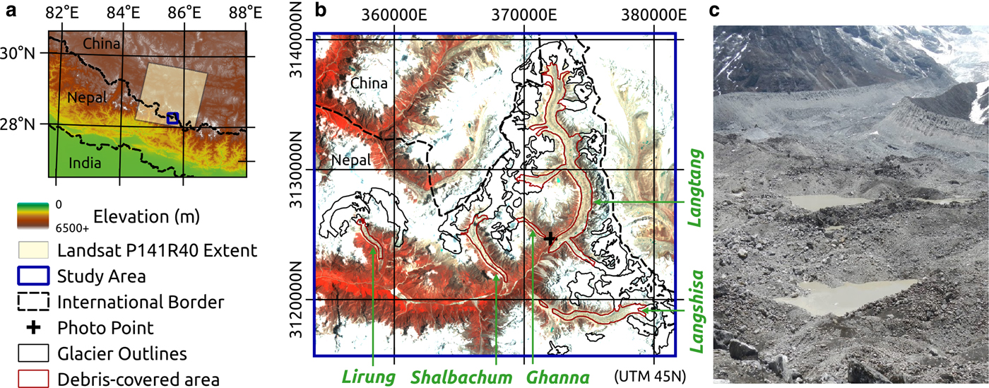
Fig. 1. (a) Geographic context of the study area within Nepal. (b) The upper Langtang basin, with the principal debris-covered glaciers identified. Backdrop is 6S-corrected Landsat TM false-color composite from 16 June 2009. (c) Photo taken 24 May 2013 near the terminus of Langtang Glacier (position at ‘Photo Point’), showing high-turbidity ponds and extremely variable relief of up to 50 m.
With an area of 350 km2, the upper Langtang catchment is 34% glacierized, with 28% of the glacier area mantled by heterogeneous rock debris, primarily covering the tongues of five valley glaciers. The debris-covered tongues are characterized by extremely variable surface relief, with large depressions occasionally filled by ponds or punctuated abruptly by bare-ice cliffs (Fig. 1c). The debris mantle varies in thickness up to at least 2.5 m (Ragettli and others, Reference Ragettli2015), composed of grains ranging in size from silt to large boulders. Lirung Glacier has been the site of numerous field studies of supraglacial ponds (Sakai and others, Reference Sakai, Takeuchi, Fujita and Nakawo2000; Bhatt and others, Reference Bhatt, Masuzawa, Yamamoto and Takeuchi2007; Takeuchi and others, Reference Takeuchi, Sakai, Shiro, Fujita and Masayoshi2012; Miles and others, Reference Miles2016) in spite of its small size and advanced decay (Immerzeel and others, Reference Immerzeel2014a). The much larger Langtang, Langshisa and Shalbachum Glaciers also show significant supraglacial ponded areas (Pellicciotti and others, Reference Pellicciotti2015), while the small Ghanna Glacier has few glaciological observations of any kind. The recent study of Ragettli and others (Reference Ragettli, Bolch and Pellicciotti2016) analysed surface thinning of these glaciers for 1974–2015, and found that the glaciers have rapidly downwasted (mean of − 1.01 m a−1 for the debris-covered area, 2006–09) but show a low rate of area change (−0.04 to −0.40% a−1).
The five study glaciers differ strongly in size, debris cover and hypsometry (Table 1). In terms of size, they range from 1.3 km2 (Ghanna) to 52.8 km2 (Langtang), with debris mantling 22% (Lirung) to 40% (Ghanna) of total glacier area. The glaciers also vary in their altitudinal extents, with terminus elevations ranging from 4025 m.a.s.l. (Lirung) to 4718 m.a.s.l (Ghanna). All five glaciers are rapidly losing mass in response to climate change. Ghanna Glacier is retreating from its terminal moraines, with Lirung and Langshisa Glaciers also retreating to a lesser degree, while Shalbachum and Langtang Glaciers are downwasting with nearly stable termini (Ragettli and others, Reference Ragettli, Bolch and Pellicciotti2016). Field observations have noted the pronounced disconnect between the debris-covered tongue and clean-ice upper portion of Lirung Glacier, a process, which has recently been noted for Shalbachum Glacier as well. Langshisa and Langtang Glaciers have both lost connectivity with minor tributaries since the 1970s.
Table 1. Comparison of morphometric and dynamic characteristics with pond observations for the five debris-covered glaciers in the study area
Elevation values correspond to the debris-covered area of the glaciers. AAR is the accumulation area ratio, while DRAA is the portion of debris-cover below the ELA. Width and DGM (elevation difference between glacier surface and moraine peaks) values are derived from profiles near the glacier terminus. Surface gradient and velocity values are the mean over the debris-covered area. Pond cover is reported as a percent of the debris-covered area and calculated as the mean value for May–October for all years. r s is the Spearman rank-order coefficient and p < 0.05 for |r s| > 0.8 since there are five glaciers.
To examine many relatively small lakes at seasonal timescales and for an extended period, the spatial and temporal resolution of observations and the length of satellite record all must be taken into account. Due to their 30 m spatial resolution, long history of repeat-visits, and free availability, the Landsat 5 (TM sensor) and 7 (ETM+ sensor) satellites offered the most promise to resolve seasonal and annual patterns of supraglacial ponds. Spectral coverage is nearly identical for the TM and ETM+ sensors (Chander and others, Reference Chander, Markham and Helder2009), although the ETM+ sensor also collects broadband panchromatic observations at 15 m ground resolution. All available TM and ETM+ observations for WRS-2 path 141, row 40 within the period 1999–2013 were retrieved from the US Geological Survey.
Landsat 5 and 7 have a return-period of 16 d, but the sensors are unable to penetrate clouds so data availability for the study site is reduced. A total of 198 scenes were identified for processing, although 26 scenes were later removed due to heavy cloud cover obscuring more than 50% of the basin's debris-covered glacier area. The scenes were cropped to the extent of the upper Langtang Valley. The temporal distribution of processed scenes is displayed in Figure 2, showing the reduced number of observations during the monsoon due to cloud cover, and the slightly lower data availability for the earlier part of the study period.
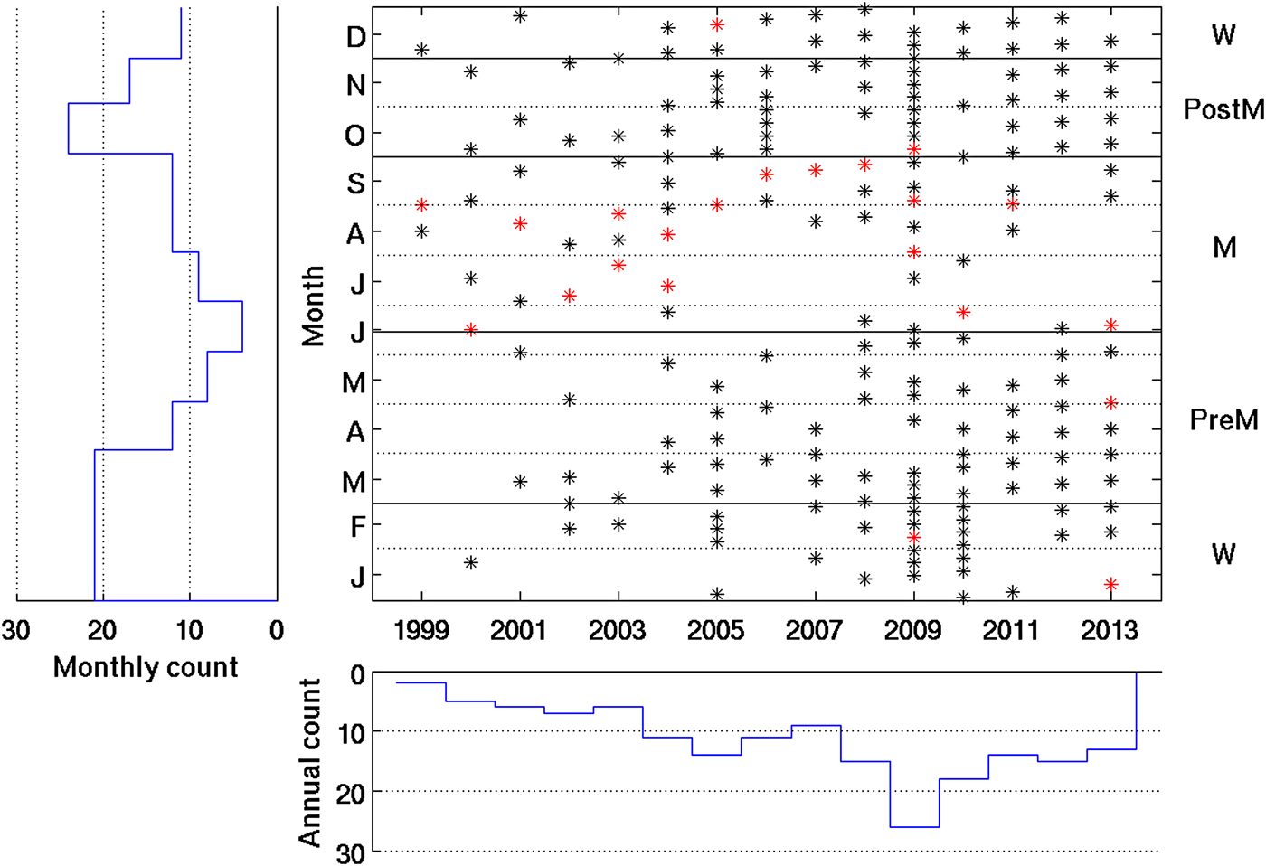
Fig. 2. Temporal distribution of scenes processed in the study, with histograms indicating monthly (left) and annual (bottom) counts of observations. Red marks are those scenes with <50% debris-covered area observable, which were removed from the analysis (26 removed from 198 scenes processed). Black marks are the scenes used in the analysis (n = 172).
Several ancillary datasets were used to analyse and interpret the Landsat data. The hole-filled CGIAR SRTM-CSI 4.1 digital elevation model (SRTM DEM), based on data collected in 2000 and gridded at 90 m resolution (Jarvis and others, Reference Jarvis, Reuter, Nelson and Guevara2008), was bilinearly resampled to the Landsat 30 m resolution to describe topography at the study site. The extents of the main glaciers and their debris-covered areas were mapped for 1999 by Pellicciotti and others (Reference Pellicciotti2015). For the present study, these outlines were supplemented by an outline for the smaller Ghanna Glacier based on the same 1999 scene. Glacier surface velocities were derived using an advanced cross-correlation methodology following Dehecq and others (Reference Dehecq, Gourmelen and Trouve2015) for 1999–2001 using Landsat ETM+ panchromatic imagery to produce annual velocity estimates: all suitable image-pairs were preprocessed for feature enhancement with an image gradient calculation, then image-pairs were fused through a spatio-temporal median filter to produce a robust estimate of annual surface velocity.
3. METHODOLOGY
We first follow a pond identification workflow to identify ponds in each Landsat scene. The differences in pond density between glaciers are then assessed with a suite of glacier morphometric characteristics; these characteristics are also used to assess the controls on ponding based on the precise positions of ponds.
3.1. Pond identification
The determination of ponded water from Landsat data required a sophisticated workflow, with the basic steps depicted in Figure 3a. An advanced atmospheric transfer code was applied to bring the scenes into close radiometric agreement (Fig. 3b), then masks for clouds, shadows and snow/ice were applied to reduce misidentification of ponds (Fig. 3c). Finally, a set of image morphological operations was developed based on band metrics to classify water objects (Fig. 3d), which were clipped to the debris-covered glacier area (Fig. 3e).
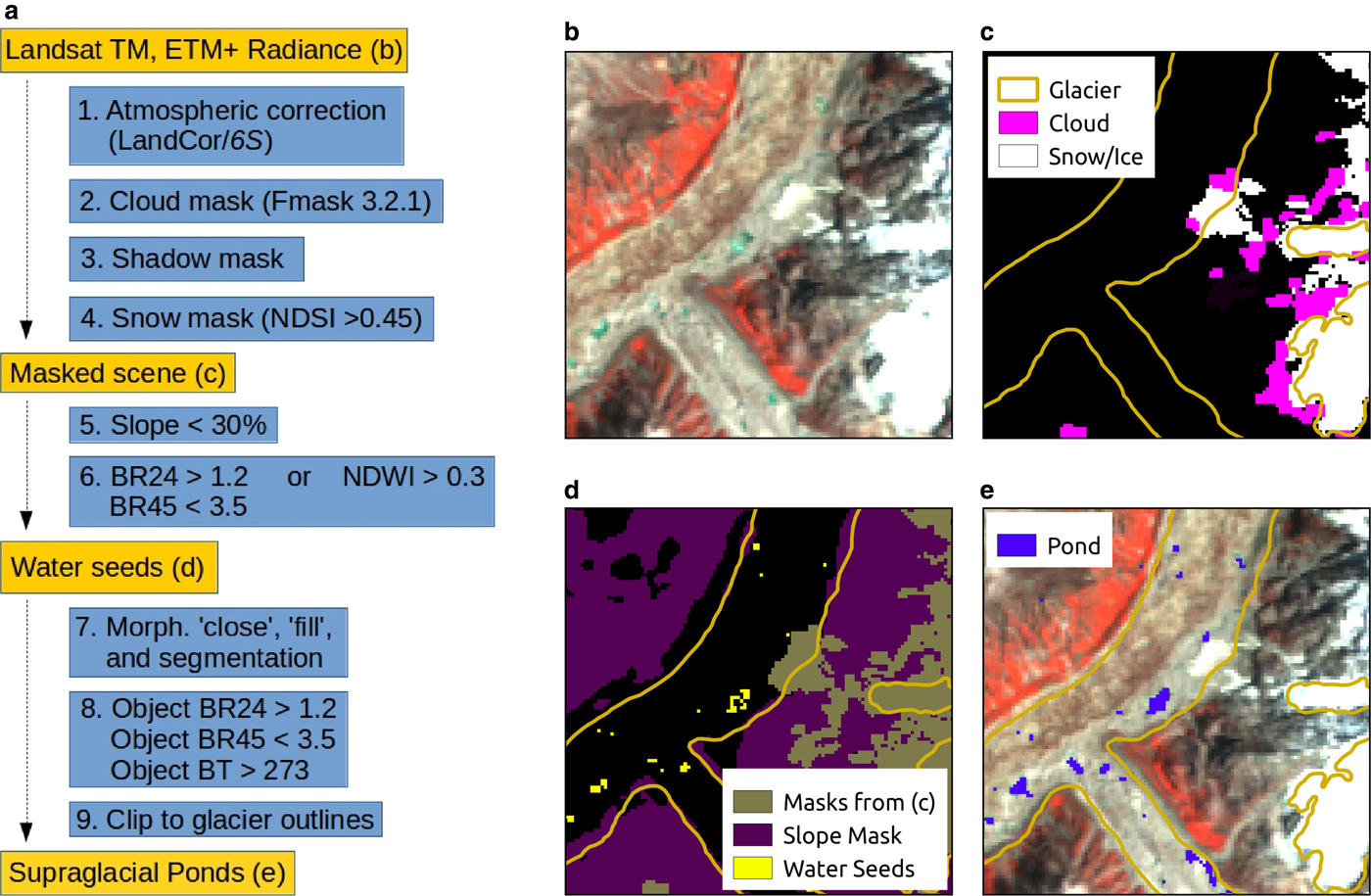
Fig. 3. (a) Processing workflow for supraglacial pond classification, with intermediate steps shown in insets (b)–(e). (b) Subset of Landsat TM false-color composite for 19 August 2009 after Landcor/6S processing. (c) Cloud, snow/ice and shadow (not shown) masks determined by subroutines, showing some difficulty with cloud identification. (d) Slope mask and determination of high-probability water seeds. (e) Pond cover output after image morphological operations and reclassification.
3.1.1. Atmospheric correction
Previous efforts to map supraglacial ponds (Gardelle and others, Reference Gardelle, Arnaud and Berthier2011; Xin and others, Reference Xin, Shiyin, Han, Jian and Qiao2011; Salerno and others, Reference Salerno2012) selected ‘ideal’ scenes with very clear atmospheric conditions and minimal snowcover to obtain snapshots of pond cover for a few time periods. These studies mapped ponds using manual thresholds of band metrics based on sensor digital numbers or top-of-atmosphere reflectance values (level 1b, geocorrected but with no radiometric correction), an approach that is straightforward and justified for a few ‘ideal’ scenes, but inappropriate for a larger number of scenes when atmospheric conditions are variable. As our study sought to take into account all potential pond observations, a robust and semi-automated method was required to bring the range of scenes into radiometric agreement, enabling accurate detection of pond cover changes by accounting for differences in sun-scene-sensor geometry and atmospheric conditions (Chander and others, Reference Chander, Markham and Helder2009).
The radiative transfer code 6S (Kotchenova and others, Reference Kotchenova, Vermote, Matarrese and Klemm2006; Kotchenova and Vermote, Reference Kotchenova and Vermote2007) has been widely used to correct for atmospheric and geometric differences between datasets (e.g. Burns and Nolin, Reference Burns and Nolin2014; Pope and others, Reference Pope2016), but is computationally taxing for an entire scene because it runs on a pixel-by-pixel basis and requires substantial data preparation. Instead, the version 4.0 Landcor code (http://www.eci.ox.ac.uk/research/ecodynamics/landcor/) was applied to the 198 Landsat scenes selected for processing (Step 1 in Fig. 3a), providing a computationally economical implementation of 6S. This code utilized metadata supplied with the raw Landsat data, including fundamental sensor characteristics (e.g. spacecraft identity, swath width, ground resolution, band spectral information) and scene-specific values, to define the illumination characteristics (e.g. scene-centre geographic coordinates, solar position, date and time) across the scene. Supplied with an atmospheric specification, Landcor developed representative lookup tables to span conditions across a scene. These lookup tables were processed with 6S and inverted to distribute corrected top-of-atmosphere reflectance values across each entire scene (Zelazowski and others, Reference Zelazowski, Sayer, Thomas and Grainger2011).
The 6S required specification of three principal atmospheric constituents: aerosol optical depth (AOD), total water vapour (TWV) and ozone (O3). For AOD and TWV, we used the findings of a previous Landcor project, which uses a topography-dependent background constituent specification and determines constituent anomalies from each scene's characteristics via an inverse approach (Zelazowski and others, Reference Zelazowski, Sayer, Thomas and Grainger2011). The values for O3 were interpolated from a daily 1-degree LEDAPS (Masek and others, Reference Masek2012) dataset developed from Total Ozone Mapping Spectrometer (TOMS) measurements spanning 1978–2011, with missing values interpolated from monthly averages computed for 2000–11.
With the full atmospheric composition and illumination geometry described for each entire scene, Landcor routines were used to: (1) prepare representative lookup-tables spanning the multidimensional space of geometry, atmospheric conditions and top-of-atmosphere spectral reflectance values; (2) run 6S for the representative cases; and (3) invert the 6S results to produce a coverage of ‘corrected’ reflectance values for each band, equivalent to a band-specific albedo. These corrected reflectance values were used for all subsequent calculations (e.g. in Fig. 3b).
3.1.2. Cloud, shadow and snow masks
The Landsat data analysed included several scenes that were affected by cloud cover, deep shadows (Chen and others, Reference Chen, Fukui, Doko and Gu2013) and seasonal snowcover, all of which required masking. The Fmask algorithm, version 3.2.1 (Zhu and others, Reference Zhu, Wang and Woodcock2015), was applied to detect clouds spanning several spectral classes semi-automatically (Step 2 in Fig. 3a).
At sites with very steep terrain, persistent shadows can be problematic for automated classification routines based on thresholds (Chen and others, Reference Chen, Fukui, Doko and Gu2013). For this study, we detected shadows in the scene based on the Fmask results, 6S-corrected TM/ETM+ band 1 and band 5 reflectance values and terrain slope. The Fmask algorithm consistently classified all terrain-cast shadows as either cloud shadows or clear water. We trimmed these two data categories to the areas satisfying B1 < 0.2 and B5 < 0.2, then performed morphological fill and close operations on connected pixel groups (more than 20 pixels) to create potential shadow coverages. As terrain shadows cover high-slope areas, each connected group of pixels was evaluated based on slope values within the group. If more than 20% of the group's pixels exceeded a 30% slope, the group was considered a shadow and removed from the potential area for pond identification (Step 3 in Fig. 3a). Shadows identified in this manner occupied up to 15% of the study area's debris-covered glaciers in December–January, but 0.6% of this area in May–October on average due to solar angle differences. Conversely, cloud effects were minimal for winter months, but affected 9.2% of the debris-covered glacier area during the May–October period.
Finally, pond surfaces may be obscured by snow in parts of the scene. Consequently, the determination of snowcover was a critical step for interpreting the pond distribution maps. The close inter-scene radiometric agreement of 6S-corrected reflectance values enabled a uniform threshold of the Normalized Difference Snow Index (NDSI = (B2 − B5)/(B2 + B5)) to be applied. Based on the cumulative NDSI histogram of all scenes, pixels were classified as snow and ice where NDSI > 0.45 (Step 4 in Fig. 3a).
3.1.3. Pond classification
Prior efforts to identify supraglacial ponds on debris-covered glaciers have used band metrics (Huggel and others, Reference Huggel, Kääb, Haeberli and Teysseire2002; Wessels and others, Reference Wessels, Kargel and Kieffer2002; Gardelle and others, Reference Gardelle, Arnaud and Berthier2011; Chen and others, Reference Chen, Fukui, Doko and Gu2013) or image morphological operations (Panday and others, Reference Panday, Bulley, Haritashya, Ghimire, Thakur, Singh, Ramanathan, Prasad and Gossel2012; Liu and others, Reference Liu, Mayer and Liu2015; Watson and others, Reference Watson, Quincey, Carrivick and Smith2016), while studies of debris-covered glaciers in general also use values of thermal band derived brightness temperature (BT) to classify glacier facies (e.g. Mihalcea and others, Reference Mihalcea2008). Our study applied a set of image morphological operations and band algebra to identify potential water bodies, then evaluated and classified them based on these metrics. The spectral metrics used were the Normalized Difference Water Index (NDWI = (B2 − B4)/(B2 + B4)), the green-to-near-infrared ratio (BR24 = B2/B4) and the near-to-middle-infrared ratio (BR45 = B4/B5). The NDWI and BR24 are both useful for differentiating between moisture (ice, snow, water) and non-moisture (rock, vegetation) landcover types, while BR45 is useful to distinguish between moisture phases.
Ponds are known to form only in areas of low surface gradient (<10°), but studies differ in the critical slope threshold used to determine the area of a debris-covered glacier conducive to ponding (Reynolds, Reference Reynolds2000; Quincey and others, Reference Quincey2007; Gardelle and others, Reference Gardelle, Arnaud and Berthier2011; Sakai, Reference Sakai2012; Chen and others, Reference Chen, Fukui, Doko and Gu2013). Due to the coarse spatial resolution of the SRTM DEM and the rugged surface of the debris-covered glaciers in the study area, which is especially pronounced near supraglacial ponds, we did not use a slope filter to restrict pond classification (Fig. 1b, Step 5 in Fig. 3a). We instead use a higher surface slope threshold of 30% to eliminate steep avalanche fans or icefalls from the debris-covered area in which ponds can form.
Using the 6S-corrected reflectance values, pond seeds were identified as locations that met the slope threshold as well as BR24 > 1.2 and BR45 < 3.5, or NDWI > 0.3, following an approach similar to Gardelle and others (Reference Gardelle, Arnaud and Berthier2011). The thresholds were initially chosen based on the thresholds identified in Wessels and others (Reference Wessels, Kargel and Kieffer2002) for ASTER data, combined with investigations of the spectral characteristics of easily recognizable lakes at the study site. The thresholds were then tested and modified through an iterative trial-and-error approach applied to all scenes to eliminate misclassified zones of saturated snow while correctly classifying known lakes.
The high-likelihood pond seeds were morphologically closed (sequential binary dilation and erosion) using a 2-pixel disk, then morphologically filled, to identify connected regions of high pond likelihood. The closing and filling operations connected adjacent areas of high pond probability, which occurred in the larger sediment-laden water bodies and spectrally variable areas of melting snow near the firn line, but not for the small isolated ponds. Connected groups of pixels were then classified based on the mean metric values for each connected body (same BR24, BR45 and NDWI thresholds as before and additionally BT > 273 K), eliminating most debris-marginal zones and creating a coverage of thawed water bodies (Fig. 3e).
Finally, the debris-covered area was determined for the 1999 glacier coverage of Pellicciotti and others (Reference Pellicciotti2015), supplemented with the outline of Ghanna Glacier. The full set of classified scenes was used to determine the glacier area that was snowfree for at least 50% of the monsoon observations, when snowcover is at its annual minimum. This debris-covered area then defined the area of analysis for supraglacial ponds over the study period (Fig. 4). Although the glaciers are undergoing rapid thinning, the areal changes of the debris-covered portion have been <0.1% a−1 in recent years, with the exception of Ghanna Glacier, which is losing area at 0.4% a−1 (Ragettli and others, Reference Ragettli, Bolch and Pellicciotti2016). We therefore treat the debris-covered glacier area as fixed for the purposes of this study.
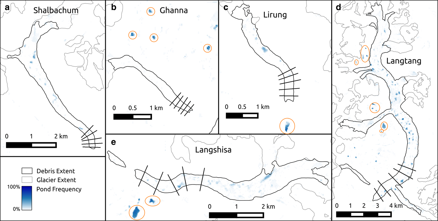
Fig. 4. Spatial distribution of supraglacial ponds as percent of May–October observations (n = 68), also showing results for other lakes outside the debris-covered tongues (orange ellipses), 1999–2013. Cross-glacier transects used for measurement of glacier width and DGM are shown as black lines.
3.1.4. Uncertainty
The pond classification results presented below are affected by several potential sources of uncertainty that are difficult to quantify. First, although the 6S radiative transfer code improves the inter-scene radiometric consistency, it relies on extrapolated and modelled atmospheric conditions and is unlikely to result in exact comparability of scenes. Second, the separation of cloud, shadow, snow and open water relies on several manually-chosen thresholds, resulting in potential misclassification of individual pixels and pond objects. Third, to distinguish between frozen and thawed pond objects, the method utilizes BT data that are of lower spatial resolution than the visible imagery (all data are provided at 30 m resolution, but thermal data are collected at 120 m for TM and 60 m for ETM+) and they are not adjusted by 6S. As ponds occur at smaller scales, this method is likely to increase sub-pixel and adjacency effects (Gardelle and others, Reference Gardelle, Arnaud and Berthier2011; Salerno and others, Reference Salerno2012; Liu and others, Reference Liu, Mayer and Liu2015; Watson and others, Reference Watson, Quincey, Carrivick and Smith2016). Finally, most pond identification approaches have difficulty with the high turbidity, small size and variable characteristics of supraglacial ponds (e.g. Wessels and others, Reference Wessels, Kargel and Kieffer2002; Bhatt and others, Reference Bhatt, Masuzawa, Yamamoto and Takeuchi2007) and the use of fixed thresholds for BR24, BR45 and NDWI may have misclassified some features in spite of atmospheric correction. These four factors likely lead to errors of commission for features spectrally similar to ponds, omission for ponds that are too small to be resolved by the sensors or are heavily sediment-laden and mixed edge effects due to the 30 m resolution of the source data.
To roughly bound these errors, we first take advantage of the log-linear size-distributions of ponds (as observed by Liu and others, Reference Liu, Mayer and Liu2015) to estimate scene-specific uncertainty. For a lower-bound estimate of pond cover, we determine the percent cover only for ponds that are at least four pixels in size, comparable with the values reported by Liu and others (Reference Liu, Mayer and Liu2015). For the upper bound, we fit the glacier-specific size-distributions for each scene to a power function (Eqn (1)), where N is the number of ponds in the size-class centred at S, and b and β are the fitted coefficient and exponent. Assuming the ponds are roughly circular, the area A in each size class may be estimated from Eqn (2). We integrate this between the minimum observable pond size (S min, 30 m) and the smallest potential pond size (S 0, 0 m) to estimate the area of unobserved small ponds, A miss (Eqn (3)), which reduces to Eqn (4) since S min ≫ S 0.
 $$N(S) = bS^\beta $$
 $$A(S) = \displaystyle{{\pi b} \over 4}S^{\beta + 2} $$
 $$A_{{\rm miss}} = \int_{S = S_0} ^{S_{{\rm min}}} A(S)$$
 $$A_{{\rm miss}} \approx \displaystyle{{\pi b} \over {4(\beta + 1)}}(S_{{\rm min}} )^{\beta + 3} $$
A further assessment of pond identification accuracy was conducted with two Cartosat-1 panchromatic orthoimages (2.5 m resolution) available for October 2006 and November 2009 and processed by Ragettli and others (Reference Ragettli, Bolch and Pellicciotti2016). Each of these occurs in close temporal proximity (<10 d) to a cloud-free or mostly cloud-free Landsat ETM+ scene, enabling a comparison of the 30 m and 2.5 m pond observations. We analysed the pond identification error by comparing the Cartosat-1 and Landsat data for a 3.3 km2 area near the terminus of Langtang Glacier, where thawed ponds were easily recognizable in the high-resolution orthoimages. Ponds were manually digitized from the orthoimages without reference to the Landsat results to determine Landsat pond omission errors, then orthoimages were reinspected using the Landsat-identified pond locations to determine Landsat pond commission errors.
3.2. Glacier characteristics
To help interpret the pond distributions, ten descriptive metrics were evaluated for the debris-covered area of each glacier, summarized in Table 1. These metrics are compared with the glaciers' mean May–October pond density using Spearman's rank-order correlation, producing correlation coefficients r s ranging theoretically from −1 (perfect negative correlation) to +1 (perfect positive correlation). For statistical significance, p < 0.05 for |r s| > 0.8 since there are five glaciers with data (von Storch and Zwiers, Reference von Storch and Zwiers1999).
First, the total area and debris-covered area (first and second metrics) are calculated for the study glaciers, as larger glaciers have potential to grow larger ponds and more numerous ponds. Larger glaciers may also be more complex in terms of hydrologic routing, with a greater likelihood of a discontinuous englacial drainage system, as englacial conduits are exposed to intersect the surface due to sustained differential surface ablation. The total glacier area and debris-covered area are computed directly from the glacier outlines. The elevation of the debris-covered tongues may be important as it controls air temperatures and surface mass balance, so minimum and maximum elevations are determined for each study glacier based on the SRTM DEM (third and fourth metrics).
The fifth and sixth metrics describe the distribution of the glacier and debris area relative to climatic forcing. The accumulation-area ratio (AAR) is a widely-used metric that describes the portion of glacier area above the equilibrium-line altitude (ELA) at which zero mass balance is expected. We use an ELA of 5400 m based on the results of prior studies in Langtang Valley (Sugiyama and others, Reference Sugiyama, Fukui, Fujita, Tone and Yamaguchi2013; Ragettli and others, Reference Ragettli2015). We then determine a ratio describing the portion of glacier area covered by debris below the ELA, the debris ratio in the ablation area (DRAA). Both ratios range from 0 to 100%.
Seventh, we evaluate glacier width, which may limit the size to which ponds can grow, and therefore the extent to which ponds may be observable. Eighth, we determine the cumulative downwasting of the glacier surface (DGM, the difference between glacier and moraine elevations as defined by Sakai and Fujita, Reference Sakai and Fujita2010), which demonstrates the state of response to climate warming of each glacier, and could be important if thinning leads to a change in pond cover. Glacier width and DGM are determined as the average based on five transects in the lowest third of the debris-covered area, here moraines are most clearly identifiable. DGM approximates the cumulative surface lowering since the Little Ice Age, when the glacier surface was at least as high as present-day lateral moraines. It is difficult to measure due to narrow moraine peaks, coarse elevation data and the rugged topography of debris-covered glacier surfaces (Sakai and Fujita, Reference Sakai and Fujita2010). We use the minimum transect elevation for the glacier surface and the dominant outermost lateral moraine peak elevation to estimate DGM. Each profile therefore produces two estimates (one for each lateral moraine), except in cases where the lateral moraine is not separable from the valley's larger geologic structure (i.e. elevation increases monotonically outwards).
For the ninth metric, we calculate the mean surface gradient of the debris-covered areas, as surface gradient has been identified as a control on surface runoff and pond formation (Reynolds, Reference Reynolds2000; Quincey and others, Reference Quincey2007; Salerno and others, Reference Salerno2012). The gradient of a debris-covered glacier surface is difficult to assess due to the rugged topography. The estimated surface gradient from the SRTM DEM by adapting the approach of Quincey and others (Reference Quincey2007), but automating and iterating their method for suitability to glacier tributaries and to better capture changes in surface gradient. First, the lowest elevation of the glacier was identified from the DEM. Next, the glacier was divided into segments based on 100 m elevation bands and the longitudinal gradient calculation of Quincey and others (Reference Quincey2007) was performed from each segment's lowest point. To reduce dependence on the elevation step, the procedure was repeated for 200, 300, 400 and 500 m elevation bands to produce several estimates of surface gradient across the debris-covered area. Finally, the median value of these estimates was determined for each pixel, producing a composite map of longitudinal surface gradients approximating the glacier's active slope.
Last, we calculate the mean surface velocity for the debris-covered area of each glacier (tenth metric). A glacier's internal ice dynamics controls the connectivity of surface and englacial conduits through the opening of crevasses and closure of conduit entrances (Gulley and Benn, Reference Gulley and Benn2007). Mean surface velocity is a coarse indicator of the breadth of processes associated with ice creep, but may indicate whether any structural reorganization occurs, or if the study glaciers are effectively stagnant. High velocities would suggest a very dynamically active glacier, with zones of crevasse formation inhibiting pond formation (Quincey and others, Reference Quincey2007; Salerno and others, Reference Salerno2012). Conversely, very low velocities may inhibit pond formation by disabling the reorganization and closure of internal conduits, or encourage pond formation by reducing the likelihood of drainage.
3.3. Analysis of pond controls
To determine the roles that surface velocity and gradient play in controlling supraglacial pond formation, all individual pond locations were evaluated with respect to the categorization adapted by Quincey and others (Reference Quincey2007) from the work of Reynolds (Reference Reynolds2000). Quincey and others (Reference Quincey2007) segmented debris-covered glacier area into four categories based on local surface gradient and velocity to understand the likelihood of pond formation: (A) area with very low surface gradient (<2°) and very low velocity (<7.5 m a−1); (B) area with very low surface gradient and higher velocity (≥ 7.5 m a−1); (C) area with higher surface gradient (≥ 2°) and very low velocity; and (D) area with higher surface gradient and higher velocity. We therefore classified each observed pond based on the local glacier velocity and surface gradient. Then, to take into account the debris-covered area in each category, we determined the total debris-covered area, pond area and pond count for each glacier and category.
4. RESULTS AND DISCUSSION
4.1. Summary of pond observations for the basin
The spatial pattern of observed ponds is shown for the study glaciers in Figure 4. Darker spots indicate distinct pond features that occurred in a large portion of the observations, while lighter spots show areas that were occasionally covered by ponds. Langtang Glacier has the greatest ponded surface area and the features with the highest frequency of occurrence (Fig. 4d). Although some false-positive identification occurred near snow/debris transitions, our algorithm reliably identified other lakes not included in the analysis (ellipses in Fig. 4).
Considering all the study glaciers and years together, ponds cover an average of 1.40% of the basin's debris-covered area (0.39% of the total glacier area) between May and October (Table 1). A total of 7138 ponds were observed over the period of record for all scenes and glaciers combined, with the majority and highest density occurring on Langtang Glacier. The pond size distributions show a roughly linear trend on a log/log scale for both individual glaciers and the valley as a whole (Fig. 5) and the mean observed pond size was 0.0037 km2 (4.1 pixels). Most ponds were very small (5525 ponds with 4 pixels or fewer), but these ponds account for only 31% of the total ponded area over the study period.
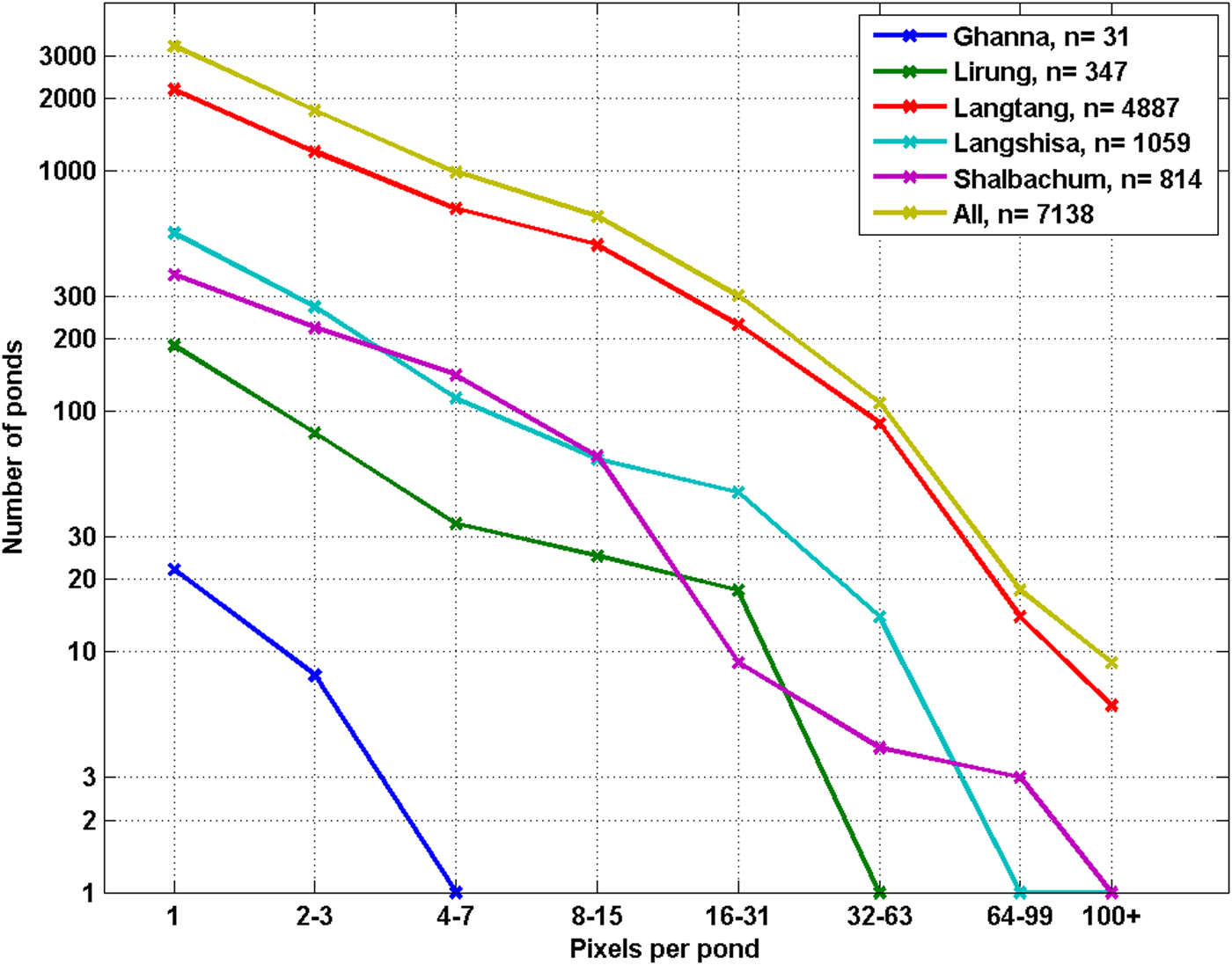
Fig. 5. Log/log plot of observed supraglacial pond size distribution for each glacier, 1999–2013. Each Landsat pixel covers 900 m2.
Our pond cover results are in general agreement with previous observations of supraglacial pond density for debris-covered glaciers. Using Landsat data, Gardelle and others (Reference Gardelle, Arnaud and Berthier2011) observed supraglacial ponds covering ~0.4% of glacier area for the Khumbu basin of Nepal, but only 0.05% for basins in the Karakoram of Pakistan, during September–October. Salerno and others (Reference Salerno2012), also studying the Khumbu basin, reported ponds covering 0.3–2% of total glacier area for individual glaciers, determined using the 10 m resolution AVNIR-2 sensor during October 2008. In contrast to our findings, that study observed a normal distribution of pond sizes. Liu and others (Reference Liu, Mayer and Liu2015), considering only ponds >4 Landsat pixels to minimize identification error, reported supraglacial ponds covering between 0.18% (1990) and 0.38% (2005) of debris-covered glacier area for their study basin in the Tian Shan of Central Asia. That study found an average pond size of 0.01 km2, which is almost exactly the value we obtained (0.011 km2, 12.4 pixels) when considering ponds of at least 4 pixels. Limiting our dataset to these larger ponds, ponds cover 0.97% of Langtang Valley's debris-covered area between May and October (0.30% of total glacier area), in very close agreement with the results of Liu and others (Reference Liu, Mayer and Liu2015) for a very different setting.
4.2. Uncertainty
Applying our statistical approach to uncertainty assessment, the size distribution suggests an overall potential commission error of 31% by area, although individual scenes varied between 0% (i.e. no small ponds were observed) and 100% (i.e. all observed ponds were smaller than 4 pixels). Estimating the omitted pond area by extrapolating and integrating scene-specific pond size distributions, we find an overall omission of <1% of pond area. However, this assessment requires that ponds are discretized in 30 m squares, and sub-pixel and boundary inaccuracies are likely to be larger than 1% (Salerno and others, Reference Salerno2012; Watson and others, Reference Watson, Quincey, Carrivick and Smith2016). Consequently, the statistical error analysis conveys lower confidence in pond identification for small features and for individual scenes, but higher confidence for larger features and for distributions of pond frequency, which highlight locations of regular pond observation.
This statistical result was further substantiated by the comparison of available high-resolution imagery with the Landsat results (Fig. 6, Table 2). The pond-identification algorithm struggles to identify small ponds of <900 m2 visible in the Cartosat-1 orthoimage (44% of features, but 7% of pond area). The algorithm performs well for ponds greater in area than 1 pixel (900 m2), in agreement with the error assessment of Salerno and others (Reference Salerno2012), but overestimates the area of these features by 30–50% due to resolution effects. The algorithm occasionally misidentified features as thawed ponds (16% of Landsat features, 2.1% of observed area); these were recognizable as exposed ice cliffs or frozen pond surfaces in the orthoimages. The combined effects of small pond omission, occasional pond commission and large-feature overestimation led to a combined error of 35% of pond area for the zone of comparison (Table 3). Given the limited comparison with high-resolution data, it is unclear how transferable these error values are to the rest of the time series as both scenes available for comparison occurred in the post-monsoon. Overall, the results are biased to larger ponds due to Landsat's 30 m spatial resolution, but the omission of small ponds is much <15–88%, as hypothesized by Watson and others (Reference Watson, Quincey, Carrivick and Smith2016), and is compensated by the misidentification of pond area at boundaries.
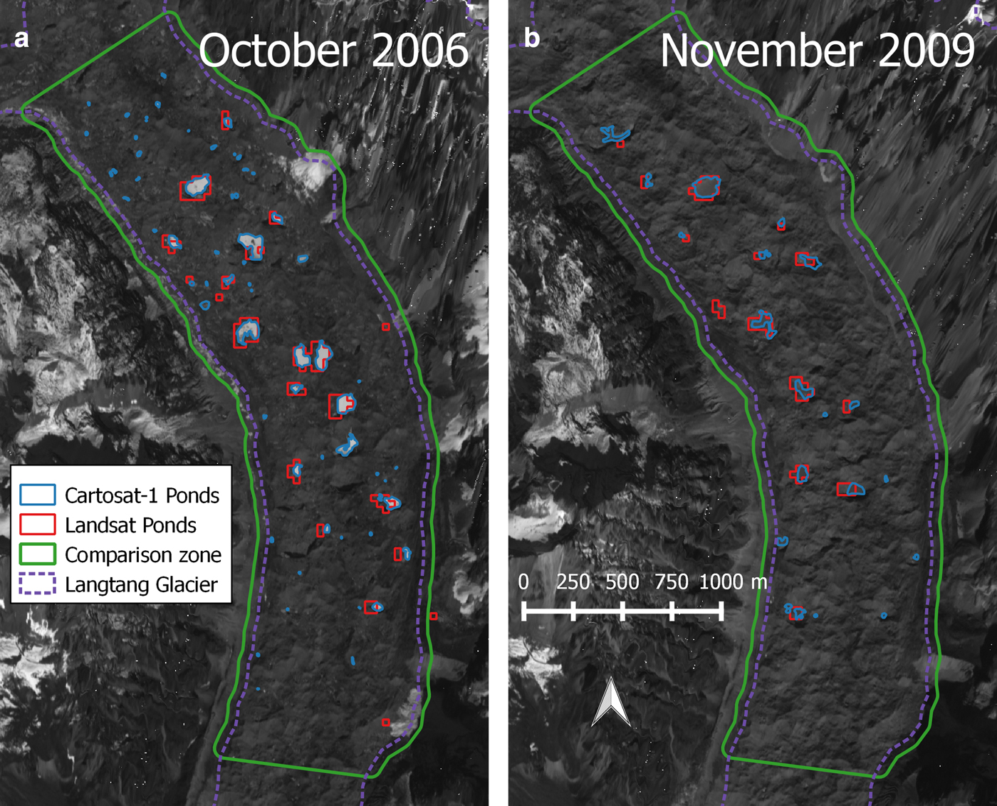
Fig. 6. Comparison of features identified by Landsat ETM+ and Cartosat-1 for October 2006 and November 2009, showing strong agreement between the datasets. Landsat misses small ponds and occasionally misidentifies pond features. The 30 m resolution is the dominant source of error for the Landsat routine.
Table 2. Landsat ETM+ and Cartosat-1 pond observations for a 3.03 km2 area of Langtang Glacier (Fig. 6)
Ponds observed in the Cartosat-1 images but obscured by SLC-error stripes are omitted. Pond sizes are reported for ponds common to both images (Observed) and for ponds not identified by the Landsat routines (Missed). Pond density for the area of comparison falls into the overall range observed by Landsat for October–November (Fig. 10, left).
Table 3. Landsat commission and omission rates of pond features and size for each scene comparison, and the overall error in pond area for each scene
Last, the analysis was hampered by the 16 d return interval of the Landsat TM and ETM+ observations, which occasionally led to several-month gaps in observations (Fig. 2). The return period also prevented observation of dynamic hydrologic processes operating on short timescales. Field observations in May 2013 indicated widespread hydrologic activity on the surface of Langtang Glacier (Fig. 7), with depressions suddenly filling and connecting via overland and englacial flow. Unfortunately, the Landsat record did not contain a cloud-free observation of the site during this period, missing the peak annual supraglacial ponding altogether.
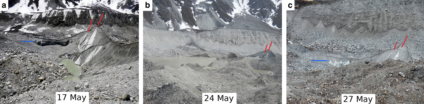
Fig. 7. An example of rapid pond filling and draining during the late pre-monsoon of 2013, at 4560 m.a.s.l. on Langtang Glacier (location indicated on Fig. 11). Blue lines indicate the approximate filled water level as seen in the 24 May photo (b), with red markers identifying recognizable clean patches on the ice cliff. Observations on 17 May (a) had found a 400 m2 pond in a 5900 m2 depression ringed with ice cliffs. By 24 May (b), in the absence of any precipitation, the depression had flooded to overflowing, which also filled adjacent depressions for a total pond area of 30 000 m2. Two days later (c), following a 14 h rainfall event, the pond had drained, leaving the subaqueous portion of the ice cliff clean.
4.3. Glacier characteristics and pond cover
The debris-covered areas of the study glaciers show significant variability in pond cover, ranging from 0.08% (Ghanna) to 1.69% (Langtang) of the debris-covered area during May–October (Table 1). The study glaciers exhibit a wide range of geometric and dynamic conditions. Glaciers in the Langtang Valley range in total area from 1.3 to 52.8 km2, while the debris-covered portion of the glaciers ranges in size from 0.6 km2 (Ghanna) to 17.8 km2 (Langtang). Only Shalbachum and Lirung Glaciers extend below 4400 m.a.s.l., while only Lirung Glacier has a mean elevation for the debris-covered area below 4600 m.a.s.l. The glaciers smallest by area also have the smallest moraine-to-moraine widths (295–970 m). The glaciers have downwasted to different degrees, with mean DGM values ranging from 30 m for Shalbachum Glacier to 125 m for Langshisa Glacier.
The study glaciers' debris-covered areas all have mean surface gradients below 10°, a threshold identified by Reynolds (Reference Reynolds2000) as being conducive to the formation of dispersed ponds. Only Langtang and Langshisa Glaciers exhibit a mean surface gradient below 6°, but none of the glaciers has an average surface gradient below 2°. Langshisa, Shalbachum and Langtang Glaciers have the highest mean surface velocities (7.9, 5.3 and 4.8 m a−1, respectively), while Ghanna and Lirung Glaciers have very low average values (0.9 and 1.5 m a−1, respectively), suggesting that portions of their debris-covered tongue are nearly stagnant.
Of the ten glacier characteristics tested at the individual-glacier scale, mean pond cover (% debris area) exhibited the strongest rank-order correlations with glacier area (r s = 1.0), debris area (r s = 1.0), width (r s = 0.90), mean slope (r s = −0.90) and DRAA (r s = −0.8). With data for only five glaciers, p < 0.05 for |r s| > 0.8 (von Storch and Zwiers, Reference von Storch and Zwiers1999). No significant rank-order relationship was found for mean velocity (r s = 0.70), glacier minimum or mean elevation (r s = −0.10 and 0.7), AAR (r s = 0.15), or DGM (r s = 0.30). For our study glaciers, pond cover is greater for the larger glaciers, those with low surface gradient, and those with a larger portion of debris-free terrain below the ELA. These relationships are tentative results based on a small sample size that could be tested with a larger set of glaciers across the region and in other regions to better understand distributions of supraglacial ponding.
Reynolds (Reference Reynolds2000) proposed a basic classification of glaciers based on their surface gradient. Glaciers with gradients in the range 2°–6° are expected to experience widespread dispersed ponding, with those in the range 6°–10° expected to exhibit isolated small ponds. These categories fit our study glaciers fairly well, with Langshisa (0.88% pond cover) and Langtang (1.69%) Glaciers in the first category, and Ghanna Glacier (0.06%) clearly in the second category. In contrast to the categories of Reynolds (Reference Reynolds2000), Lirung and Shalbachum Glaciers have high mean surface gradients (10.2° and 7.1°) and exhibit moderate pond cover (0.57 and 0.73%). For both of these glaciers, the standard deviation of velocity over the debris-covered area is nearly equal to the mean, suggesting a relatively strong decay down-glacier, and potentially a zone of longitudinal compression. If this is the case, crevasses and relict conduits may be forced to close, and only hydrofracture is likely to enable pond drainage (Benn and others, Reference Benn, Gulley, Luckman, Adamek and Glowacki2009).
If progressive thinning increases pond density as the glacier surface approaches the hydrological base level, as may be expected immediately prior to formation of a terminal lake, DGM would show a relationship with pond cover. In our results, however, DGM explains very little of the variability in ponding between glaciers. First, apparent ponding may not increase dramatically until the hydrological base level is nearly reached, so cumulative thinning may not exhibit a clear relationship with pond formation. Second, Sakai and Fujita (Reference Sakai and Fujita2010) found that large terminal lakes were more likely to form if DGM exceeds 50 m and the terminus surface gradient is below 2°. Although high DGM values were obtained for Langshisa, Lirung and Langtang Glaciers, the 2° surface gradient condition is not met for any of the study glaciers, and none of the study glaciers exhibits a terminal lake or shows signs of increased water storage near the terminus. Rather, it appears that all ponds identified in the study are ‘perched’ above the hydrological base level.
4.4. Pond spatial distributions and controls
Surface velocities and gradients derived for the five debris-covered tongues are shown in Figure 8. The five glaciers show distinct patterns of surface velocity, with widespread near-stagnant areas. Langshisa, Langtang and Shalbachum Glaciers all show a pattern of strong velocity decay through their debris-covered tongues (i.e. longitudinal compression), but show very low surface velocities for the terminal 1.5, 8 and 2 km, respectively. Lirung and Ghanna Glaciers have very little area moving faster than 5 m a−1, although Lirung Glacier is known to show seasonal fluctuations in surface velocity (Kraaijenbrink and others, Reference Kraaijenbrink2016).
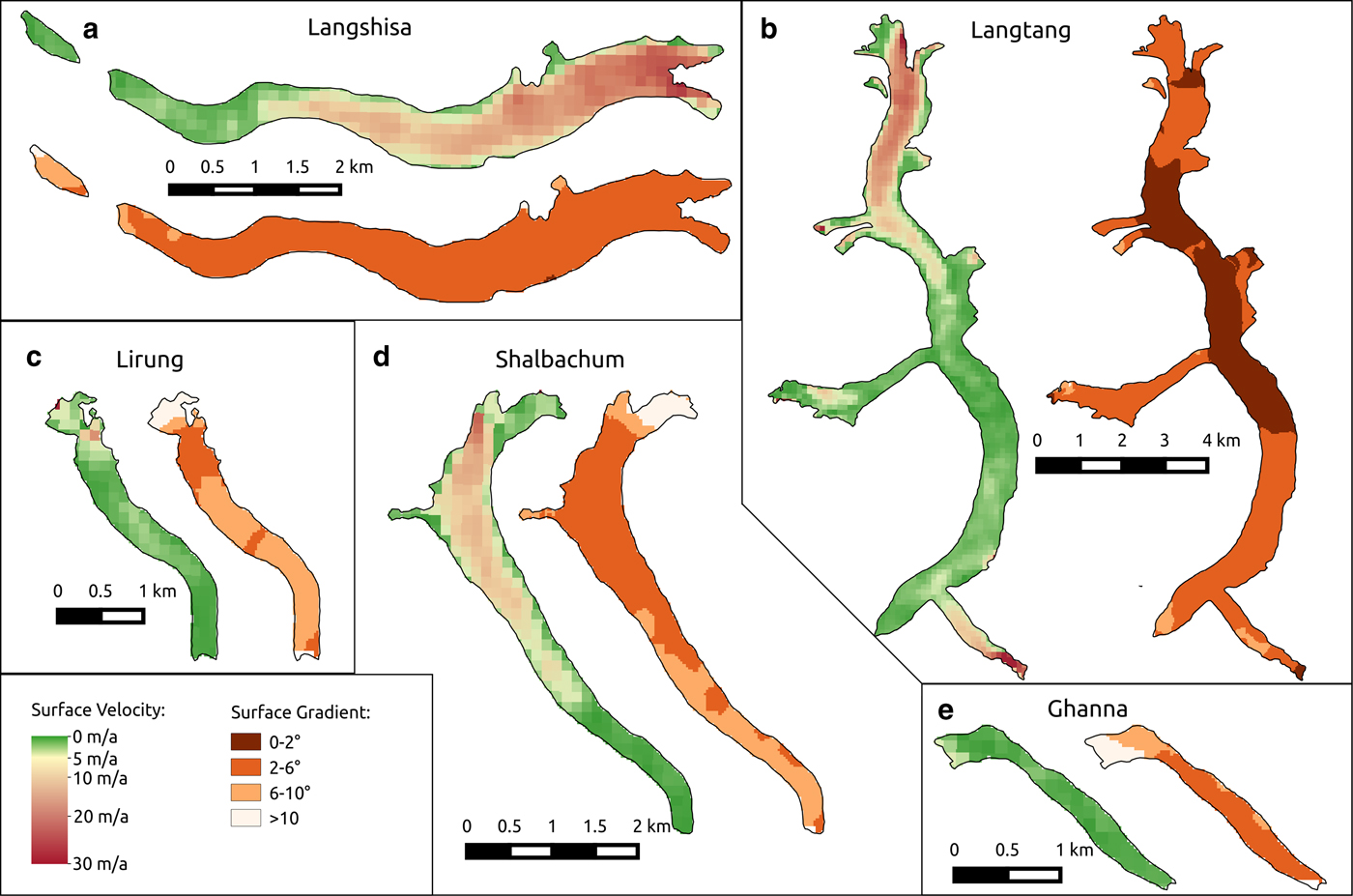
Fig. 8. Annual velocity and surface gradient for the debris-covered areas of the study glaciers. Annual velocity was derived using the method of Dehecq and others (Reference Dehecq, Gourmelen and Trouve2015) but with Landsat ETM+ panchromatic data (band 8). Surface gradient was derived by a method similar to Quincey and others (Reference Quincey2007).
The debris-covered tongues of the five glaciers also show differing patterns of surface gradient. Langshisa Glacier has a surface gradient almost entirely in the 2° − 6° range, only exceeding 6° at its terminus. Of the five study glaciers, only Langtang Glacier shows any area with a surface gradient below 2°, which occurs for a large central portion of the glacier's tongue. Langtang also shows very little area with a surface gradient higher than 6°. Most of the surface of Lirung Glacier has a gradient above 6°, while a few small portions of the glacier exhibit gradients between 2° and 6°, mostly near the valley headwall. Most of Shalbachum Glacier is in the 2° − 6° surface gradient range, although the lower 3 km and the upper 1 km both show surface gradients above 6°. Ghanna Glacier shows nearly the opposite pattern: a steeper upper portion (>6°), with most of the tongue falling in the 2° − 6° range.
Ponds are present in all four categories identified by Quincey and others (Reference Quincey2007), but appear to be more frequent in zones of lower velocity and lower surface gradient (category A, Fig. 9). Langtang Glacier dominates the overall distribution of ponds (68% of ponds) as it has the largest area and highest pond density. It is also the only glacier to exhibit all four of the categories, as none of the other four glaciers have surface gradients below 2° anywhere on their debris-covered tongues.
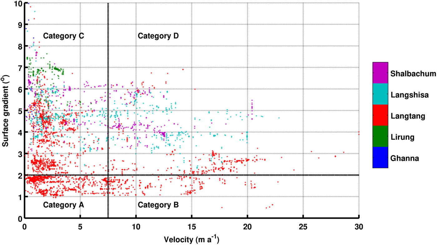
Fig. 9. Distribution of local surface gradient and velocity for all observed ponds, with marker size indicating the number of pixels for each pond. Categories A–D correspond to Table 4 and Quincey and others (Reference Quincey2007).
Comparing the total portion of debris-covered area and ponded area within each category produces an estimate of the density of ponds in each zone (Table 4). Here, it becomes clear that although only 19.6% of the Langtang Valley's debris-covered glacier area is classified as Category A (low gradient, low velocity), this zone accounts for 36% of the observed supraglacial pond area over the period of record; this category has the highest density of ponds (2.99% by area, 5.9 features per km2). Category B (low gradient, high velocity) encompasses the smallest portion of the debris-covered area (5.9%) and pond area (5.2%), for the second-highest density of ponds (1.42% by area, 5.0 features per km2). Third-highest in terms of pond density is Category C (high gradient, low velocity), which describes the majority of the debris-covered area (52.9%) but just under half of the observed pond area (44.3%), leading to a lower density of ponds (1.36% by area, 3.7 features per km2). For Category C, there is moderate variability in the pond density between glaciers but no glacier approaches the relative density of Category A. Finally, Category D (high gradient, high velocity) shows the lowest density of ponds (1.09% by area, 3.6 features per km2), encompassing 21.6% of debris-covered area but only 18.3% of pond area. The variability between glaciers within Category D is also moderate but density values are lower than for all other categories.
Table 4. Distribution of debris area, observed pond area and count of ponds within each gradient and slope category with (–) denoting no area
The table encompasses the full period of record, so total ponded area is greater than the debris-covered glacier area in category A.
The average size of ponds in each category is also apparent from this approach. In Category A, ponds average 0.0050 km2 in area (5.6 pixels). For Category B, the average pond size is 0.0029 km2 (3.2 pixels). Ponds in Category C average 0.0037 km2 (4.1 pixels), while those in Category D average 0.0031 km2 (3.4 pixels). The average pond sizes for each category are very consistent between glaciers.
According to these results, pond density seems to increase with lower surface gradients and lower glacier velocities, with surface gradient showing the stronger control. Pond size, though, seems to increase only with lower velocities, showing a mixed relationship with surface gradient. Our results are in general agreement with the findings of Quincey and others (Reference Quincey2007), but in contrast to that study, we find numerous smaller ponds in Category B, instead of the potential for a few large ponds. Also, in Category C and D we find a greater portion of ponds than expected, nearly on par with Category B relative to the respective debris areas.
In synthesis, we are in agreement with the framework of Reynolds (Reference Reynolds2000) and Quincey and others (Reference Quincey2007) that surface gradient exerts a primary control on pond formation by determining the likelihood of surface water accumulation. We argue that surface velocity exerts a secondary control on pond formation, because the zones that experience heightened velocity and ponding also show a strong down-glacier deceleration (Fig. 8), and this compressive flow may discourage drainage via englacial conduits, rerouting meltwater onto the glacier surface. However, surface velocity exerts a strong control on pond persistence by encouraging connectivity between the supraglacial and englacial hydrologic systems. Thus, when ponds do form in zones of moderate velocity they are typically smaller, because the higher local velocity provides more opportunity for drainage.
4.5. Pond seasonality
We assessed the seasonality of thawed ponds in the Langtang Valley according to the seasonal definitions of Immerzeel and others (Reference Immerzeel, Petersen, Ragettli and Pellicciotti2014b) to determine the period and magnitude of surface ponding as relevant to the glaciers' surface energy balance and ablation (Fig. 10, left). The frozen surface of ponds in winter is often difficult to distinguish from snow drifts, which also accumulate in the surface depressions, a spectral separation that is especially challenging with the spatial resolution of Landsat data. Ponds with a frozen surface layer were therefore discounted from the analysis presented here, but would be important to observe from a hydrologic perspective.
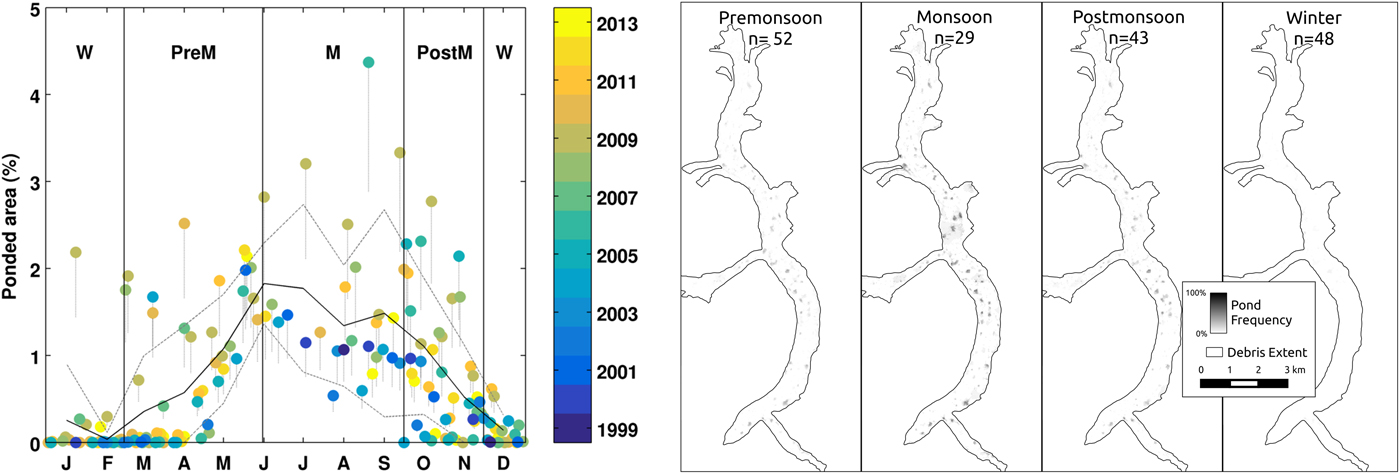
Fig. 10. Seasonal pattern of thawed pond cover as percent of observable debris-covered glacier area (left), with individual scenes coloured by year of observation (n = 172) and dot tails highlighting the effect of a 34% overestimation of pond area. The solid black line is the monthly mean, with dashed lines showing the ± 1σ spread. The seasonal pattern is demonstrated by pond frequency maps derived from all data for each season (right), highlighting the widespread prevalence of ponds during the monsoon. This panel shows only Langtang Glacier for space considerations.
Considering thawed ponds only, supraglacial pond cover in the Langtang valley shows an increase during the pre-monsoon, rises to a peak in the early monsoon, drops during the post-monsoon and decreases to negligible during the winter months (Fig. 10, left). The seasonal pattern is highlighted by aggregate maps of the pond frequency for each season for Langtang Glacier (Fig. 10, right). During the pre-monsoon, ponds are more frequent on the lowest portions of the debris-covered tongue. Ponds are very common in the monsoon and distributed across all elevations (Fig. 10, right). Fewer ponds are apparent during the post-monsoon, and very few ponds were observed in winter, as the water surface freezes for a large portion of the year (Fig. 10, right).
Several authors have suggested a strong seasonality of pond cover (Takeuchi and others, Reference Takeuchi, Sakai, Shiro, Fujita and Masayoshi2012; Liu and others, Reference Liu, Mayer and Liu2015) due to the seasonal peak in the ablation process and its controls on englacial conduit opening and closure (Reynolds, Reference Reynolds2000; Sakai and others, Reference Sakai, Takeuchi, Fujita and Nakawo2000). Our observations generally support these earlier ideas. There is a reduction in snowcover in the pre-monsoon as temperatures rise (Benn and others, Reference Benn2012), leading to the uncovering and thawing of ponds frozen over winter and the filling of surface depressions without an englacial drainage outlet, especially at lower elevations. During this period, thawed ponds increase in cover to peak at the onset of the monsoon at 2% of the glaciers' debris-covered area. The greatest hydrologic flux occurs during the monsoon due to the combination of high melt rates and rainfall, with snowmelt providing the greatest source of water (Ragettli and others, Reference Ragettli2015). During this period, pond cover declines slightly to 1–1.5% of debris-covered area. Fewer ponds remain in the post-monsoon, and thawed pond cover rapidly diminishes due to decreasing temperatures and declining water supply. Very cold temperatures and occasional snowfall occur in the winter, and any remaining ponds freeze and may be obscured by snow.
The seasonal delivery of surface water to the interiors of the glaciers via pond drainage has important implications for mass balance and for glacier dynamics. Ponds efficiently absorb energy at the surface (Sakai and others, Reference Sakai, Takeuchi, Fujita and Nakawo2000; Miles and others, Reference Miles2016), so drainage can lead to heightened internal ablation along englacial conduits (Benn and others, Reference Benn2012; Thompson and others, Reference Thompson, Benn, Mertes and Luckman2016). Seasonal variations in surface velocity could also be closely tied to pond seasonality as an expression of increased basal lubrication and sliding (Kraaijenbrink and others, Reference Kraaijenbrink2016), while such a change in glacier dynamics can hinder or encourage drainage from the surface to englacial or subglacial networks (e.g. Gulley and others, Reference Gulley, Benn, Screaton and Martin2009).
4.6. Pond persistence, recurrence and evolution
Supraglacial ponds often persist for several years before an englacial connection develops, while in other cases ponds recur as the same depressions refill after drainage points become blocked (Benn and others, Reference Benn, Wiseman and Hands2001; Immerzeel and others, Reference Immerzeel2014a). Unfortunately, due to the sporadic temporal coverage of the Landsat record it is difficult to distinguish between pond persistence and recurrence. Both are important, and for different reasons: pond persistence (i.e. longevity or duration) controls the local effects that water at the glacier's surface may have (e.g. calving, subaqueous melt, sedimentation, debris reorganization), while pond recurrence directly relates to a pond's effects in the glacier's interior (the frequency with which it conveys atmospheric energy via drainage). Here we analyse the repeated pond occurrences, which could indicate either persistence or recurrence.
To highlight the persistence and recurrence of ponds, we examine pond frequency maps (Figs 4, 10). Langtang and Lirung Glaciers have very persistent or recurring pond locations even over the 15-year study period (identifiable as darker spots), while ponds on the faster-flowing Shalbachum and Langshisa Glaciers tend to be shorter-lived (showing as lighter smears). To highlight persistence and recurrence over shorter periods, pond-frequency maps were computed for three 5-year windows within the study period: 1999–2003, 2004–08, and 2009–13 (Fig. 11). Here, individual ponds can be readily identified as features with higher frequency, and lake emergence, expansion and disappearance processes are evident over the 15-year period. The 5-year pond frequency plots are useful for examining longer-term patterns in pond cover in a discrete manner, and show that the general distribution of ponds has not changed substantially, although the persistence or recurrence of ponds may change over time as outlined below.
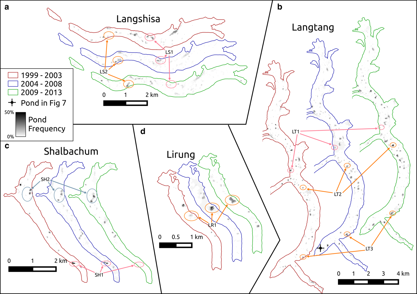
Fig. 11. Distribution of supraglacial ponds as percent of cloud-free debris-covered glacier area for 5-year subsets, highlighting the increase in overall ponded area and the persistence of individual ponds. Ghanna Glacier is not shown due to its lack of pond cover. The colour scale is limited to 50% for clarity, but the 5-year windows had maximum May–October pond frequency values of 91, 72 and 81% for 1999–2003, 2004–08 and 2009–13, respectively.
In some cases, a location showing persistent or recurrent ponding for the early period decays slowly, showing a decreased area and frequency for the middle period before disappearing entirely (see LS1, SH1 and LT1 in Fig. 11). In other cases, areas of ponding expand or emerge and are very frequently observed for the later period (see LT2 and LT3 in Fig. 11b). More complex cases are also apparent: on Lirung Glacier, a pond system (LR1 in Fig. 11d) becomes much more frequent during the middle period and then both expands and becomes less frequent for the latter period. This pond has also been observed to fill and drain semi-regularly in field observations. Pond system SH2 (Fig. 11c) shows even more complex behaviour. In the early period, two individual persistent ponds are very apparent high in the debris-covered area. For the middle period, the same ponds are evident but are less frequent, and another pond is evident nearby. By the third period, all three locations have been slightly advected down-glacier and the uppermost location rarely shows ponding, while the lower two locations show frequent ponding and are occasionally connected.
Over the entire study period, 29.4% of the debris-covered glacier area shows ponding in at least one scene, with 45% of this area observed twice, suggesting that a large proportion of ponds show persistence and recurrence. Furthermore, 40.5% of the ponded area was identified as a pond in 2 or more years, while 8.9% of the ponded area was identified as a pond in at least 5 years. Similarly, persistent and recurrent ponds accounted for 25–50% of all supraglacial ponds in consecutive years in the Khan Tengri mountains (Liu and others, Reference Liu, Mayer and Liu2015).
Pond persistence and recurrence, as indicated by the portion of area identified as a pond in 2 or more years, was higher for surface categories A and C (low velocity, 48 and 41%, respectively) than for categories B and D (higher velocity, 35 and 31%, respectively). As the debris-covered tongues continue to downwaste and stagnate, a shift to lower gradient, lower-velocity surfaces may lead not only to higher pond densities and larger ponds, but also to increased pond persistence and recurrence.
4.7. Interannual variability
Changes in pond cover on the multiannual (Liu and others, Reference Liu, Mayer and Liu2015) and decadal (Gardelle and others, Reference Gardelle, Arnaud and Berthier2011) timescales are a key point of interest, as a potential indicator and feedback for glacier response to climate warming (Benn and others, Reference Benn2012) and as an early warning for the formation of proglacial lakes (Bolch and others, Reference Bolch, Buchroithner, Peters, Baessler and Bajracharya2008). A key objective of this study was therefore to determine whether an increase in supraglacial ponded area has occurred over the study period. However, satellite observations of supraglacial ponds are severely limited by sporadic cloud cover and seasonal snowcover, as well as the failure of the Landsat 7 Scan Line Corrector in 2003. Furthermore there is a marked seasonality of pond cover, with high pond cover occurring during the monsoon when cloud cover is very common, and minimum pond cover occurring in winter when cloud free images are numerous, but many lakes are obscured by snow. A multi-year investigation of ponding variability must account for these effects before a pattern can be assessed.
To remove biases of cloud and snowcover, we selected all scenes for each glacier where more than 80% of the debris-covered area was observable and where < $10\% $
of that observable area was covered by snow. We then aggregated the pond cover data into annual time series for each season: the pre-monsoon emergence and filling of ponds, the high monsoon pond cover and the post-monsoon decline in pond cover associated with pond drainage (Fig. 10, left). For each season and year with data, we computed the mean and standard deviation of pond cover for each debris-covered glacier and scene to reduce sampling biases.
$10\% $
of that observable area was covered by snow. We then aggregated the pond cover data into annual time series for each season: the pre-monsoon emergence and filling of ponds, the high monsoon pond cover and the post-monsoon decline in pond cover associated with pond drainage (Fig. 10, left). For each season and year with data, we computed the mean and standard deviation of pond cover for each debris-covered glacier and scene to reduce sampling biases.
After applying the data quality filters, only Langtang Glacier's debris-covered area is observable in a moderate number of scenes for all three seasons. No trend in pond cover is apparent from the multi-year data for any season for this glacier (Fig. 12, left). Pond density was lower in 1999–2005 than 2006–13, but the increase in scenes after 2005 also coincides with an increased spread of pond density values. Consequently, the picture is not one of sustained increase over the 15-year study period, but rather of moderate interannual variability for all seasons, accompanied by moderate changes in pond density within seasons.
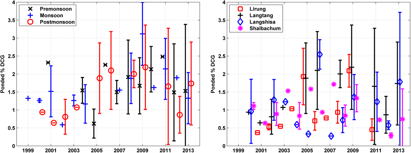
Fig. 12. Interannual pattern of supraglacial ponding by season for Langtang Glacier, showing the mean ±1σ expressed as percent of observable debris-covered glacier area (left). Post-monsoon interannual variability of supraglacial ponding at the four larger glaciers, showing the mean ±1σ expressed as percent of observable debris-covered glacier area (right). For both panels, data included have at least 80% of the debris area visible and <10% covered by snow.
The post-monsoon has the highest density of scenes during the portion of the year when ponds are thawed (Fig. 2) and is comparable with the periods of analysis of Gardelle and others (Reference Gardelle, Arnaud and Berthier2011) and Liu and others (Reference Liu, Mayer and Liu2015). Due to the better scene coverage, the interannual variability of Lirung, Langshisa and Shalbachum Glaciers was also investigated for this season (Fig. 12, right). The mean ponded areas for these four glaciers showed marked variability over the study period, with pond cover varying between 0.2% and 4% of debris-covered area. None of the glaciers have a consistent pattern of ponding, instead showing multiple peaks and falls, and high variability for any year (Fig. 12, right).
The interannual variability in pond cover for each glacier could be related to interannual variability in key meteorological conditions controlling the timing and supply of water to fill the surface depressions. Considerable interannual variability in ponded area was also observed by Liu and others (Reference Liu, Mayer and Liu2015) in the Tian Shan, and was related to total ablation season precipitation and antecedent temperatures. For our study site, analyses of seasonal temperatures, seasonal precipitation, preceding annual positive degree days, preceding annual cumulative precipitation did not reveal clear patterns of links between pond cover and meteorology (not shown). Conversely, Gardelle and others (Reference Gardelle, Arnaud and Berthier2011) noted an increase in supraglacial ponded area for the Everest region over their 29-year study period, but relied on only three Landsat scenes, all from the post-monsoon.
Notably, the glaciers and years with multiple observations do not show close agreement, suggesting that important changes in surface ponding occur at the glacier scale even within a short-time window. This is a challenge for a multi-year analysis: it is not clear whether the observations of Gardelle and others (Reference Gardelle, Arnaud and Berthier2011) and Liu and others (Reference Liu, Mayer and Liu2015) were affected by the seasonality and rapid variability of pond cover demonstrated by this study, and a better understanding of the temporal variability of supraglacial ponds is needed.
5. CONCLUSIONS
Our analysis of the spatial and temporal variability of supraglacial ponds in the Langtang Valley, Nepal, uses a robust radiometric correction and pond identification methodology applied to five debris-covered glaciers and spanning 15 years of observation to build upon and substantiate the current understanding of the distribution of these features. This study uses many more observations than previous efforts but generally supports inferences that were drawn by Reynolds (Reference Reynolds2000); Quincey and others (Reference Quincey2007); Salerno and others (Reference Salerno2012); Liu and others (Reference Liu, Mayer and Liu2015) that pond incidence is strongly controlled by local surface gradient and glacier velocity. Surface gradient controls water accumulation (i.e. pond formation) while velocity controls pond drainage and therefore pond size and persistence. We find that ponds are most concentrated and largest in zones of low surface gradient (<2°) and low velocity (<7.5 m a−1), where water is likely to accumulate and ponds are unlikely to drain. Ponds are nearly as common but smallest in zones of low gradient but higher velocity, as they are more likely to drain. Ponds are less common but large in zones of moderate gradient and low velocity, as they may persist longer and have the opportunity to expand. Finally, ponds are least common and are small for zones of moderate gradient and velocity.
In addition we make several novel contributions to the current understanding of supraglacial ponds:
-
(1) We make the first systematic observations of the seasonality of supraglacial ponds on debris-covered glaciers, finding that thawed ponds cover 1–2% of the basin's debris-covered area for May–October. Pond cover rises rapidly in the pre-monsoon as ponds thaw and seasonal snowmelts, peaking at ~2% of the basin's debris-covered area at the onset of the monsoon. Pond cover then gradually declines through the monsoon as ponds drain by establishing connectivity with the englacial hydrologic system, and ponds continue to drain and many freeze over during the post-monsoon. The seasonal patterns of pond cover have important implications for assessments of glacier mass balance and hydrology (e.g. Ragettli and others, Reference Ragettli2015) as these features absorb atmospheric and radiative energy at a high rate (Sakai and others, Reference Sakai, Takeuchi, Fujita and Nakawo2000; Miles and others, Reference Miles2016). As climate warms in High Mountain Asia, the seasonal timing of supraglacial ponds may change, driven by earlier or stronger meltwater supply and the glacier surface conditions may become more conducive to ponding as deceleration and downwasting continue (Benn and others, Reference Benn2012).
-
(2) Seasonal pond dynamics reveal potential biases in basic assessments of ponded area change, such as those relying on only a few observations. We do not find a trend in pond cover for Langtang Glacier in pre-monsoon, monsoon, or post-monsoon periods. Langtang, Langshisa, Shalbachum and Lirung Glaciers all exhibit marked interannual variability of pond cover, with pond cover varying year-to-year between 0.2% and 4% of debris-covered area for the post-monsoon period. Use of fewer scenes could lead to strongly differing conclusions concerning pond growth, stability, or decline due to signal aliasing. This underlines the importance of using a numerous, seasonally-distributed set of satellite observations for change detection of processes that fluctuate on a seasonal scale.
-
(3) We find that supraglacial ponding varies strongly between glaciers in the relatively small upper Langtang Valley catchment, ranging from 0.06 to 1.69% of debris-covered area for May–October mean values. The magnitude of ponding is most related to glacier size and surface gradient. Pond cover does not show a statistically-significant relationship with cumulative glacier thinning, or with whole-glacier mean surface velocity. A similar interglacier comparison of pond cover is recommended for an expanded set of glaciers to evaluate the consistency of these relationships between basic glacier characteristics and surface ponding in this and other regions.
-
(4) We find that persistent and recurrent ponds are commonplace on the four larger glaciers, with 40.5% of all pond locations observed in multiple years. Notably, many locations appear to persist or recur for the entire analysis, suggesting that individual pond features may have a prolonged effect on the debris-covered surface and englacial conduits.
-
(5) Rather than a steady change in pond cover, the glaciers exhibit high interannual variability in ponding, with multiple peaks and falls over the study period, and high variability for all seasons.
One stimulus for research into supraglacial pond cover stems from glacier hazards and the possibility of formation of large moraine-dammed lakes. Lirung, Shalbachum and Langshisa Glaciers are known to have been retreating since 1974 at least (Pellicciotti and others, Reference Pellicciotti2015; Ragettli and others, Reference Ragettli, Bolch and Pellicciotti2016), with Lirung Glacier having formed, and then retreated from, a small moraine-dammed lake prior to 1999. This leaves Langtang Glacier as a potential site for hazardous lake formation, and it already exhibits advanced downwasting with a DGM of 50 m. However, the intermediate gradient near the terminus (2° − 6°), low terminus pond density and interannual variability in ponding suggest that formation of a base-level lake is still many years away, if indeed it occurs at all.
Our findings suggest several avenues of research to better understand supraglacial ponding for the debris-covered glaciers of High Mountain Asia. First, observations capturing the timing of pond filling or drainage for a large area, especially during the monsoon, would greatly advance understanding of the glaciers' hydrologic system. The recent launch of Landsat 8 enables continued long-term analysis of pond cover, and the high data quality and alternating overpass schedule relative to Landsat 7 may reduce some of the spectral and temporal limitations of this study, although the limitations of 30 m spatial resolution will pose a continued challenge. A study of pond distributions leveraging higher-resolution orthoimagery would constrain the moderate commission error of this study, but would need to take the seasonal variability of ponds into consideration. Finally, pond persistence and recurrence are difficult to distinguish but are useful concepts for understanding the effects of supraglacial ponds at the glacier surface and englacially, and should be investigated further through detailed field studies encompassing a domain of moderate extent to quantify the dynamic behaviour of supraglacial ponds.
ACKNOWLEDGEMENTS
This study was made possible by the high-quality surface velocity data generously provided by Amaury Dehecq. We would like to acknowledge Przemek Zelazowski for his hard work improving LandCor. We are thankful to Allen Pope for field help in May 2013. We would like to thank numerous collaborators at ETH-Zürich and ICIMOD for fruitful discussions and scientific support, and Tek Rai and his team for their outstanding fieldwork support. We would also like to thank reviewers Liu Qiao and David Rounce for excellent comments and questions, and Chief Editor Graham Cogley for his careful reading and suggestions, all of which have greatly improved the manuscript.


 Open access