


Introduction
Water at the bed of a glacier exerts critical control on temporal variations in basal sliding and hence in glacier surface velocity (e.g. Reference Hooke, Brzozowski and BrongeHooke and others, 1983, Reference Hooke, Calla, Holmlund, Nilsson and Stroeven1989;Reference Iken, Rothlisberger, Flotron and HaeberliIken and others, 1983; Reference Hanson and HookeHanson and Hooke, 1994; Reference Kamb, Engelhardt, Fahnestock, Humphrey, Meier and StoneKamb and others, 1994; Reference MeierMeier and others, 1994; Reference Harper, Humphrey, Pfeffer and WelchHarper and others, 1996b; Reference Iken and TrufferIken and Truffer, 1997). Most temperate glaciers show the highest sliding velocities in the early spring and summer (Reference Iken, Rothlisberger, Flotron and HaeberliIken and others, 1983; Reference Harper, Humphrey and PfefferHarper and others, 2003). Superimposed on increased summer motion are short-period (a few days) velocity events that can occur at any time during the melt season. Times of high surface velocity are usually associated with periods of rapid surface melt, drainage of water stored in supraglacial lakes or intense rainfall events. When documented, diurnal variability in sliding often lags behind the meltwater inputs (e.g. Reference WillisWillis, 1995). That water at the bed of temperate glaciers exerts control on basal motion is therefore clear; what is less well understood is how sliding evolves in space (across the entire glacier bed) and time (over the balance year) as a function of a changing basal hydrologic system. Because subglacial erosion is so strongly tied to basal sliding, understanding the controls on sliding is important for geomorphic models of alpine landscape evolution (e.g. Reference Harbor, Hallet and RaymondHarbor and others, 1988; Reference Braun, Zwartz and TomkinBraun and others, 1999; Reference MacGregor, Anderson, Anderson and Wadding-MacGregor and others, 2000; Reference TomkinTomkin, 2003).
The state of the basal hydrologic system plays an important role in setting both the amount of water that can be stored at the glacier sole, and the basal sliding rates (e.g. Reference Iken and BindschadlerIken and Bindschadler, 1986). Numerical modeling by Reference IkenIken (1981) suggests that glacier velocity is likely to be high during the initial, transient stages of subglacial cavity growth, when cavities are small (early spring). Iken hypothesized that once the cavities have enlarged due to sliding, more water is needed to pressurize the cavities and therefore sliding is not easily induced. Reference Iken and TrufferIken and Truffer (1997) infer that while high pressure can be maintained in isolated cavities without affecting glacier sliding at Findelengletscher, Switzerland, cavities that are better connected will cover a larger proportion of the glacier bed, and will promote a tighter connection between water pressure and glacial sliding. Development of conduit networks, which transport water rapidly to the glacier terminus, occur later in the melt season as increasing melt rates increase the volume of water within the glacier. We expect the spatial and temporal distribution of ‘slow’-flow cavities and ‘fast’-flow conduits to control not only the timing and magnitude of water discharge from glaciers, but the distribution of water pressures at the bed (e.g. Reference Fountain and WalderFountain and Walder, 1998). The effect of the evolution of the glacial hydrologic system on the spatial and temporal distribution of basal sliding has been explored in detail only rarely (e.g. Reference Iken, Rothlisberger, Flotron and HaeberliIken and others, 1983; Reference Iken and BindschadlerIken and Bindschadler, 1986; Reference CochranCochran, 1995; Reference Mair, Nienow, Willis and SharpMair and others, 2001). These studies focused on changes in the subglacial drainage architecture in one portion of a glacier, with interpretations based on sparse surface velocity measurements.
In an effort to gain insight into the seasonal, glacier-wide pattern of basal motion, we documented the spatial and temporal evolution of surface velocity on a small temperate valley glacier over the course of two summer melt seasons. We present velocity data for both years of measurement, and estimate enhanced basal sliding, as others have done, by subtracting measured winter surface velocities (assuming they are proxies for depth-integrated internal deformation and any steady component of regelation-based sliding) from the surface velocity field. Using measured snow and ice melt, and water discharge, we construct a basin-integrated water balance, and examine its relationship with basal motion and surface uplift. We interpret records of basal motion and surface uplift in terms of the evolution of subglacial hydrologic conditions over the melt season.
Field Location
Bench Glacier
Bench Glacier is a temperate alpine glacier located in the Chugach Range, south-central Alaska, USA, 30 km east of the town of Valdez, and 50 km northeast of Prince William Sound (Fig. 1). Bench Glacier was selected for its relatively simple geometry, its accessibility and its small size. In 2000, the glacier was 7 km long, averaged 1 km in width and had a total surface area of ~7.5 km2. The glacier flows to the north-northwest, from 1625 m elevation at the highest col to 940 m at the terminus. In the ablation zone, the glacier slopes gently at 5°, steepening to 11° at the terminus. At 4-5 km from the terminus, a crevassed icefall is present on the eastern side of the glacier. Above this icefall the accumulation area has a lower mean slope, with rolling topography on the order of 400 m wavelength and 20 m amplitude, and is somewhat crevassed. The average equilibrium-line altitude (ELA) at Bench Glacier is ~-1500m.

Fig. 1. (a) Map of Bench Glacier. Glacier surface topography mapped using global positioning system (GPS) in July 2000. Approximate location of the ELA (~1500 m) is shown by the dashed black line. (b) Longitudinal profile of Bench Glacier from ice radar (black triangles), GPS (gray triangles) and US Geological Survey topographic map (black dots). Estimates of ice thickness 4-7 km from the present terminus were made using measured surface slope and assuming a shear stress of 1 bar.
The bedrock geology is a fairly uniform late-Cretaceous Valdez Group meta-greywacke (Reference Winkler, Silberman, Grantz, Miller and MacKevettWinkler and others, 1981), dipping ~30-40° N (down-glacier). Thin (~1-2m) discontinuous till and supraglacially derived debris mantles the majority of the lower valley walls. Till thickness under the glacier is unknown. High-resolution ice-penetrating radar across the ablation zone (Reference MacGregorMacGregor, 2002), along with borehole videotapes and borehole penetrometer tests in 2002, suggest that till cover is spotty, and that the bed is not mantled by a thick till layer (personal communication from J. Reference Harper, Humphrey and PfefferHarper, 2003).
Methods
The data presented here were collected between May 1999 and September 2000. Four visits covered 16 weeks in the field: 24 May-13 July 1999, 11-22 September 1999, 8 June-9 July 2000 and 9-30 August 2000.
Ice thickness
In June 1999, 14 radar transects were measured on Bench Glacier using the radar system of Reference Welch, Pfeffer, Harper and HumphreyWelch and others (1998) (see also Reference Narod and ClarkeNarod and Clarke, 1994). Resolution is approximately ±10 m (Reference Welch, Pfeffer, Harper and HumphreyWelch and others, 1998). Maximum ice thickness of 185 m occurs 3.5 km from the 2000 terminus (Fig. 1).
Ice surface motion
Surface motion was determined using both traditional optical survey techniques (both summers) and differential global positioning system (DGPS) (in 2000). In 1999, we installed seventeen velocity stakes, nine along the glacier center line, and eight additional stakes defining two crossglacier profiles (Fig. 1). In 2000, we added five velocity stakes in the accumulation zone (stakes 10-14). The 2000 stakes were placed within 20-180 m of their 1999 counterparts. A Total Station located on the bedrock ridge to the west of the glacier was used to conduct repeat measurements of the stake array. With the exception of stakes 1 and 2A-2E, prisms were delivered to and mounted on the stakes only during survey campaigns. During measurements, stakes were held vertically to correct for lean, aided by leveling devices. Continuous GPS monitoring of ice motion at one stake was conducted in 2000, in addition to the DGPS and surveying measurements.
Annual surface velocity
We determined annual surface motion at stakes 1-6 by reoccupying the September 1999 stake locations in August 2000. To determine winter velocity (October 1999- May 2000), we subtracted the displacement measured between June and August 2000. Rock cairns built at the stake locations in July 1999 were relocated in August 2000, using optical survey techniques. We estimate cairn reoccupation uncertainty to be ±50 cm, with a higher likelihood of overestimating displacement due to the down-slope motion of individual clasts.
Surface velocity (all stakes)
Stakes 1-7 were surveyed approximately twice a week. Stakes 8 and 9 were included less frequently due to accessibility problems and poor atmospheric conditions. Following Reference Harper, Humphrey, Pfeffer and WelchHarper and others (1996), we calculate an error ellipse for each stake based on angular and distance uncertainties, with shape and orientation of each ellipse dependent upon its position relative to the survey station. From this, we determined an uncertainty vector parallel to thedirection of glacier motion and used this as the calculated stake position uncertainty (Tables 1 and 2). These are maximum possible uncertainties; true errors are likely to be smaller as a result of careful and uniform instrument operation.
Table 1. Calculated uncertainties in surveyed stake location measurements

Table 2. Calculated errors for GPS fast static stake locations
The majority of stake location measurements in 2000 were made using DGPS. The base station (Trimble 4000 SSI) was installed on bedrock near the survey station. Biweekly fast static position measurements entailed reoccupation of stakes with a DGPS unit. Data were post-processed using Trimble software.
In addition, an electronic distance measurement device (EDM) station was set on a small moraine mound, about 500 m from the glacier terminus (Fig. 1). Surveying prisms attached to stake 1 and stakes 2A-2E ranged from 840 to 1125m from the EDM (340 and 600 m from the glacier terminus).Weather permitting, distance measurements to the stakes were made twice daily. These data illuminate stake motion near the terminus prior to the seasonal establishment of the glacier-wide surveying and GPS networks.
Surface velocity (stake 5)
A continuously recording static GPS station was installed at stake 5 in summer 2000 (Fig. 2). The station consisted of three steel poles drilled 3 m into snow and ice, to which a level plywood platform was attached. The GPS antenna was screwed to a bolt attached to the plywood, allowing us to reoccupy the location precisely and easily after using the unit for a DGPS survey. Gaps in the data at stake 5 represent these fast static surveys. Fifteen minutes of static data were processed to determine stake position once every 4 hours, generating a 4 hour time series of surface displacement.

Fig. 2. Average surface velocity measurements in the ablation zone during the 1999/2000 balance year. The solid black line shows annual average surface velocity between September 1999 and August 2000, which ranges between 2.3 and 3 cmd-1. Average winter velocities are slightly less than annual velocities, suggesting the majority of annual surface motion results from steady motion of the ice. Average summer velocity in 2000 was 2.7_3.8 cmd-1.
Snow thickness and melt
Snow thickness was measured using an avalanche probe across the glacier surface and ablation stakes along the glacier center line. In addition, a series of four snow pits were dug in June of each year. Snow density measurements were collected over ~-20cm intervals, and were used to convert snow loss to water equivalent units. In addition, 18-22 ablation stakes were installed across Bench Glacier (Fig. 1). Stakes were measured almost daily in the ablation zone, and less frequently, about once a week, in the accumulation zone. Uncertainty in stake length measurement is ±0.5 cm; melt rate uncertainty (based on measurement frequency) was as high as 20% but was generally <5%. Automated oblique photographs were taken from a ridge west of the glacier every 2 days to monitor snowline retreat.
On 1 May 2000, several laser altimetry profiles (Echel- Reference Echelmeyermeyer and others, 1996) were flown along the center line of the glacier. The nearest laser altimetry data point for each GPS stake location was identified using least-squares calculations. The difference between snow surface elevations on 1 May and measured ice surface elevations upon our arrival in mid-June constrains snow thickness at the time of the laser altimetry survey (i.e. pre-melt season). Vertical uncertainty of the laser altimetry system is ±20-30cm (Reference EchelmeyerEchelmeyer and others, 1996).
Water discharge
Stream stage was measured at the gauging station ~500m from the glacier terminus (Fig. 1). An acoustic lookdown sensor identical to the snowmelt sensor at the meteorological station was pulsed at 1 Hz, and was averaged and recorded at 15 min intervals. A rating curve developed using the salt dilution technique (e.g. Reference KiteKite, 1994) allowed conversion of stage to water discharge.
Results
Surface velocity
Ice surface velocity results are presented in three subsections, in order of increasing temporal resolution: (i) winter and annual surface velocity; (ii) motion along the glacier center line (measured twice daily to biweekly) and (iii) vertical and horizontal motion at a single stake (measured every 1-4 hours).
Annual surface velocity
Annual average surface velocity in the ablation zone is shown in Figure 2. In general, annual surface velocity increased with distance from the terminus, although stakes 4-6C had very similar velocities. The maximum speed was ~3cmd-1 at stake 6C, while the mean speed (stakes 1-6C) was 2.5 cm d-1. Average winter (October-May) velocities were nearer 2cmd-1. Average summer velocities were therefore 25-35% greater than winter velocities for all six stakes, presumably reflecting the contribution from enhanced summer basal motion. Summer velocities showed a clearer increase with distance from the terminus. Based on our estimated uncertainty in cairn reoccupation, uncertainties in annual surface velocity are <7%. As we were unable to reoccupy stakes 7-10 in August 2000, we cannot constrain annual velocities at and above the icefall.
Summer surface velocity
Strong spatio-temporal patterns can be seen in each year’s record of horizontal velocity (Fig. 3). In general, every stake displays a period of low surface velocity, followed by a pulse of increased velocity. Elevated velocity persists for a few days, and then gradually slows until it reattains the low velocity it had before speed-up. Our late arrival at the glacier in 2000 on day 164 (12 June) did not allow us to capture the rise to elevated velocity at stakes 1-3.

Fig. 3. Horizontal surface velocity (black lines) as a function of time in (a) 1999 and (b) 2000. The corners of the step plots are the data; horizontal lines show average velocity between measurements. Note differences in temporal windows (x axis) and velocity range (y axis) between 1999 and 2000. The horizontal dark gray bars show measured winter surface velocity (1999/2000) for each stake; these data were not collected at stake 7 and above. GPS data for stake 5 (2000) are shown in light gray.
In both summers, the pulse of elevated surface velocity began near the terminus and propagated up-glacier. In 1999, surface velocity at stakes 1-6C was 3-4 cm d-1 in early June (days 151-156). On approximately day 156, velocity increased across these stakes, with the most dramatic increase at the lower stakes, 1 and 2C. By day 159, average surface velocity at stakes 1 and 2C declined, and remained relatively low for the rest of the measurement period. Surface velocity at stake 3 reached a maximum by day 159, and was beginning to slow by day 164, as stakes 4 and 5 reached their maximum surface velocity. By day 169, stake 7 had reached its peak velocity for the season. The temporal structure at stakes 8 and 9 is similar. While it is plausible that the highest velocity at these stakes occurred after day 169, we cannot resolve this, as these stakes were measured only four or five times over the 45-day period.
A similar pattern is evident in 2000 (Fig. 3b). Increased surface velocity lasted 4-7 days at each stake, and the initiation of rapid motion propagated up-glacier over the 30 day measurement period. In both 1999 and 2000, stakes 4, 5 and 6C show very similar records; elevated velocities occur simultaneously across this portion of the glacier. While the onset and drop-off of high velocity may be sequential from stake 4 to stake 6, the temporal measurement resolution is too coarse to confirm this.
Figure 4 shows the timing of the surface velocity peak as a function of distance from the terminus. The time of peak velocity was taken to be the midpoint of the temporal window over which the highest velocity was measured. The peak in surface velocity travels from the terminus into the accumulation zone over the course of ~15days, averaging 250md-1. While this pulse of elevated surface velocity appears to have been initiated about 10days later in 2000 than in 1999, the propagation speed is very similar. The propagation speed is slightly smaller in the lower 3 km of the glacier (just under 200 m d-1) than higher on the glacier. The spatial distribution of the maximum velocity attained over the season (Fig. 4b) is similar in 1999 and 2000. Lower peak surface velocities (<10cmd-1) are attained at sites >4 km and <1.5 km from the terminus, while generally higher peak surface velocities (>10cmd-1) are achieved near the longitudinal center of the glacier. The largest difference in peak velocity between 1999 and 2000 was between stakes 5-7, with differences in peak velocity of up to 6 cm d-1.

Fig. 4. Timing (a) and magnitude (b) of peak velocity as a function of distance from the glacier terminus. Data from both 1999 and 2000 are shown (circles). (a) Timing of peak (highest) horizontal velocity as a function of distance from the glacier terminus. (b) Magnitude of peak (highest) horizontal surface velocity as a function of distance from the glacier terminus. Points not connected by line represent scatter of measured values from several stakes.
Some of the differences in the wave of surface velocity between years are artifacts of our sampling strategy. First, measurements of surface displacement were initiated later in 2000 than in 1999. Second, the history of surface motion is significantly more complex than recorded in biweekly measurements (as demonstrated with the static GPS data below). By averaging over several days of motion, we both underestimate the maximum surface velocity and exaggerate the duration of the peak velocity. The shorter time interval between location measurements in 2000 may explain why the peak velocities measured at stakes 5, 6C and 7 were much higher in 2000 than in 1999. Despite these issues, it is clear that the timing and character of the surface velocity pulse (hereafter referred to as the propagating speed-up event) was similar in both years.
High-resolution surface velocity at stake 5
Total horizontal surface displacement at stake 5 between day 165 and day 240 of 2000 was 3.2 m, yielding an average surface velocity of 3.9 cm d-1 (Fig. 5a, b). However, horizontal surface velocity at this location changed rapidly three times, and over the summer varied by almost an order of magnitude (2.8-21 cmd-1). Average horizontal velocity was determined by averaging the slope of displacement over a selected temporal window during which velocity was relatively constant (Fig. 5b). Average vertical velocities were calculated over the same time periods (Fig. 5d). The highest horizontal velocities were measured on day 167-168 and between days 176 and 180. The first period of high horizontal velocity, immediately after installation of the GPS, corresponds exactly with high velocities measured at stakes 1 and 2C, indicating that the lowest 3 km or so of the glacier moved rapidly and coherently in the short-lived velocity event during day 167-168 (Fig. 3). We have no velocity data during this time for stakes above 5, and therefore cannot determine whether more of the glacier was involved. The later propagating speed-up event passes stake 5 between days 176 and 180. It is associated locally with positive (upward) vertical velocities at stake 5, in sharp contrast with the rest of the GPS record there (Fig. 5c and d). Because stake 5 was the only static GPS site, it is the only location where high-resolution vertical motion data were obtained.

Fig. 5. (a, c) Horizontal (a) and vertical (c) displacement at stake 5 using static GPS measurements (2000 only). (b) Average horizontal velocities at stake 5. Horizontal velocity varies between 2.8 and 21 cmd-1. (d) Average vertical velocities at stake 5. Like horizontal velocity, vertical velocity shows a complex signal, with motion varying greatly from bed-parallel, including a period of surface uplift.
Summary of surface velocity data
A zone of elevated surface velocity, 2-4 times the annual average, propagated up-glacier at 200-250md-1 from the terminus into the accumulation zone in the melt seasons of both 1999 and 2000. Peak velocities were similar in the two years, although the wave was initiated about 10 days later in 2000. Limited measurements in 2000 suggest that the speedup wave extended into the accumulation zone, although probably with reduced amplitude. Velocities after this propagating speed-up event were close to winter surface velocities, particularly at stakes 3-6. In 2000, the initiation of the high-velocity wave at the terminus was accompanied by rapid horizontal motion at stake 5. This rapid motion then dropped off at stake 5, but picked up again ~8days later, reflecting the arrival of the surface velocity wave. Surface uplift, well resolved only at stake 5 in 2000, was associated with the propagating speed-up event, with highest uplift rates coinciding with rapid horizontal motion (Fig. 5).
Snowmelt
Snow densities at each pit varied by <15%, and average snow-pit density varied by <10% across the glacier each year. We calculated snowmelt in water equivalent units by determining a glacier-averaged snow density of 480 kgm-3 in 1999 and 520 kgm-3 in 2000. In 1999, limited flow (<0.2m3s-1) in the glacier outlet stream before day 160 suggests snowmelt was negligible prior to this time. Laser altimetry data suggests average melt rates in the ablation zone of 1.5-2.7 cm d-1, and ~1 cm d-1 in the accumulation zone between days 122 and 166 (2000). We have no snow density measurements prior to day 170, although it is likely that snowpack density increased between May and mid- June. Calculations of melt rates and snowpack thicknesses (in water equivalent) prior to day 166 are therefore considered maximum values.
The seasonal evolution of snow and ice loss from the glacier surface is shown in Figure 6. Typical melt rates in the ablation zone were 2-2.5 cm d-1 w.e. in June of both years. By July, melt rates near the terminus increased to 2.53.5 cmd-1, with the higher melt rates measured at stakes where ice was exposed. Between mid-July and the end of August, melt rates in the ablation zone ranged from 3.54.2 cm d-1 in 1999, but were considerably lower in 2000 (2.5-3.3 cm d-1). Melt rates in the accumulation zone (stakes 9 and above) reached a maximum of ~1-2 cm d-1. While it is likely that little melt occurred prior to the initiation of measurements in 1999, significant melt had occurred by initiation of on-site measurements (day 165) in 2000. In both years, the melt rate increased by roughly 25-50% at each ablation stake once ice was exposed at the surface. In both years, the initiation of the propagating speed-up event occurred when average snowpack thickness across the glacier (average of stakes 1-10) was 1.2-1.4mw.e. While melt rates decreased with distance up-glacier, there were no significant glacier-wide increases in melt rate during the propagating speed-up event.

Fig. 6. (a, b) Snow and ice melt in (a) 1999 and (b) 2000. Symbols are the measurements; lines connect the data for a given day of measurement. Snow and ice loss are shown in water equivalents, with loss of ice plotted as negative (below the dashed line). (c, d) Cumulative melt at several stakes in (c) 1999 and (d) 2000; steeper slopes indicate higher melt rates.We plot both years beginning with zero melt for purposes of comparison, despite melt prior to our arrival in 2000.
Snowline migration is shown in Figure 7. In 1999, the snowline at the end of the summer melt season reached ~-1550m elevation (~5-6km from the glacier terminus), while in late August 2000 the snowline reached 1300m (~4km from the terminus). This reflected higher winter snowfall in 1999/2000 than in 1998/99, as well as slightly lower melt rates in July and August 2000. Importantly, the glacier was snow-covered throughout the speed-up event in both years. Rates of snowline migration are slightly greater than those observed by Reference Nienow, Sharp and WillisNienow and others (1998) on Haut Glacier d’Arolla, Switzerland.

Fig. 7. Snowline retreat over the melt season in 1999 (circles) and 2000 (squares). The dotted lines represent the best linear fits to the data.
Glacier mass balance
Winter, summer and annual mass balance are shown in Figure 8. The winter balance in 1999 (measured in late May) was similar to the winter balance observed in mid-June 2000. In May 1999, a thick proglacial snowpack and low water discharge (<0.1 m3s-1) suggests that little melt occurred prior to our arrival. In contrast, a well-developed outlet stream with discharges of ~2m3 s-1 was present at the start of the field season in mid-June of 2000. Because significant snowmelt occurred prior to our arrival in 2000, we show a laser altimetry-based estimate of winter balance for 1999/2000 (Fig. 8b). The laser altimetry winter balance in 2000 is clearly greater than winter balance the previous year (Fig. 8a).

Fig. 8. Mass balance in (a) 1999 and (b) 2000. Data points are the solid dots, and the best-fit lines (dashed) through the data are shown. The solid vertical line shows the location of zero balance at the end of the summer. (a) Winter balance (dark gray) measured in late May; summer balance (light gray) measured in mid-September. (b) Winter balance data (dark gray) collected in the field mid-June; laser altimetry estimate of winter balance from 1 May 2000 (thick gray line). Summer balance (light gray) measured between mid-June and late August 2000.
In 1999, there are no summer balance data above 1300m, as we were unable to cross the crevassed icefall during late summer. The 2000 summer balance data are based on measurements made between mid-June and late August 2000, and therefore do not include snowmelt between 1 May (laser altimetry) and mid-June (start of field campaign). The summer balance was an average of 1.5 m more melt on the lower part of Bench Glacier in 1999 than in 2000. If we include estimated snowmelt from laser altimetry data (between 1 May and mid-June 2000), summer balance for 1999 and 2000 would be similar (not shown). Importantly, the location of the end-of-summer snowline is well constrained in both 1999 and 2000 by late-summer (August/September) measurements. Specific mass balance was approximately -1 mw.e. in 1999 and +0.1 mw.e. in 2000.
The gradient of winter balance in 1999 was 0.9 m w.e. km-1; this value was roughly doubled in 2000 (1.9 m km-1). The summer balance also differs between 1999 and 2000. The loss of snow and ice is greater in 1999, with a gradient of 3 m km-1 elevation. In 2000 the gradient is 2.7 m km-1. Total melt below 1100 m exceeded 3.5 m w.e. in 1999, but was <2.5 m in 2000. The lower July and August melt rates in 2000 were probably related both to thicker snowpack, which delayed the transition to bare-ice melt rates, and to cooler temperatures compared to 1999. The average daily temperature between days 165 and 230 was 4.5°C in 1999, and 3.5°C in 2000.
Bench Glacier net balance in 1999 was —6.25 × 10⁶m3 of water, while in 2000 it was slightly positive, at 1 × 10⁶m3. The estimated volumetric loss since 1950 is —300 × 106m3, or —6 × 10⁶m3a-1 (Reference MacGregorMacGregor, 2002), indicating that 1999 was typical of glacier health over the past half-century.
Water discharge
Typical water discharges in Bench Glacier’s outlet stream, Bench Creek, were 2-4 m3s-1, although measured discharges ranged from <0.1 to >7 m3 s-1 (Fig. 9). In 1999, water discharge showed long-period variations between 5 and 20 days (Fig. 9a). Water discharge was somewhat greater in the middle of the record (~days 210-230), although the highest recorded discharge occurred around day 262, following a very heavy late-season rainstorm. The discharge record from 2000 shows several sharp increases and decreases (Fig. 9b). The large peaks (~day 194 and ~day 217) correspond neither to intense rainfall events nor to increased surface melt. Diurnal variability in the discharge record is clear throughout the record, with daily amplitudes ranging from <0.5 to 3m3s-1. In 1999, daily amplitude gradually increased until day 220 before declining until a rainstorm event just prior to day 260. In contrast, the 2000 record shows an abrupt step on day 220 in the observed daily discharge range, from ~0.25 to ~1.5 m3 s-1. In both years, the temporal pattern of water discharge broadly follows increases and decreases in mean daily air temperature (Fig. 9).

Fig. 9. (a, b) Water discharge (gray) and mean daily air temperature (measured at ~1265m elevation, stake 6C) in (a) 1999 and (b) 2000. (c, d) Timing of daily peak water discharge (as a fraction of a day) in (c) 1999 and (d) 2000
In the spring and early summer of both years, peak discharges occurred upward of 12 hours after the peak daily melt (~1400 h) (Fig. 9c and d). In 1999, the timing of peak water discharge gradually moved to earlier in the day beginning at about day 185;by day 200 the peak occurred consistently at ~1900h. In 2000 this change was more abrupt, between days 195 and 200. These transitions in the timing of peak discharges occurred ~10-25days after completion of the propagating speed-up events.
Interpretation
Surface velocity due to internal deformation
While we have documented the surface velocity field, we are primarily interested in the pattern of basal motion. Because no boreholes were drilled during the course of this study, we infer the timing and rate of sliding by removing the component of surface speed due to internal deformation and possibly steady, regelation-related basal motion. Measured late-summer and winter displacements demonstrate negligible variation in velocity at any given stake; velocities between stakes increase smoothly with ice thickness. We use winter displacement data to determine surface motion due to internal deformation. Our calculations of basal motion are therefore minima, as it is possible that steady basal motion is contributing to our winter motion measurements. Limited documentation of winter velocity, ice thickness and surface slopes in the accumulation zone prevent reliable estimates of basal motion there.
The pattern of the variable component of basal motion, which we hereafter call sliding, is the difference between measured summer surface velocities and measured winter velocities (Fig. 3). Peak sliding velocities of 7-9 cm d-1 were similar at stakes 1, 2C and 3 in both 1999 and 2000, with greater peak velocities in 2000 at stakes 4, 5 and 6C. This may be an artifact of the shorter temporal window over which velocities were averaged in 2000. In both years, stakes 1 and 2C appear to slide in unison, as do stakes 4, 5 and 6C. Interestingly, stake 3 is sliding rapidly during periodic high sliding both below it (stakes 1-2C) and above it (stakes 4-6C).
Although velocity related solely to internal deformation could not be calculated for stakes 8-14, surface velocity data strongly suggest that the sliding velocity wave continues beyond stake 7 (Fig. 3). Because the temporal resolution is lower here than on the rest of the glacier, it is not possible to say with certainty that the wave propagates to the glacier headwall. The few previous observations of horizontal motion in a glacier accumulation zone show that seasonal variations in velocity are smaller in the accumulation zone than in the ablation zone (Reference Hooke, Calla, Holmlund, Nilsson and StroevenHooke and others, 1989).
Surface uplift (stake 5)
In general, changes in vertical (uz ) and horizontal (uxy) velocity at stake 5 occurred simultaneously. This is expected if the surface velocity vector is parallel to the bed (assuming no emergence/submergence velocity);the ratio of the vertical and horizontal speeds should equal the tangent of the mean bed slope. However, between days 176 and 180 the surface elevation of the glacier at stake 5 increases, suggesting significant deviation of the surface velocity from mean bed-parallel (Fig. 10a). Estimates of local mean bed slope, 0, at this location are 70-100 m km-1, or 0.07-0.10, based on the radar data (Fig. 1b). Depending on the bed slope assumed, the maximum surface uplift is 8-16 cm. The bed slope that best fits the data outside the speed-up event (days 166-175 and after day 190) is 0.09, while the data between days 190 and 239 suggest 0.072 (Fig. 10b).

Fig. 10. (a) Vertical and horizontal displacement measured using static GPS at stake 5. Shaded box denotes the period of high horizontal velocities and associated ice surface uplift between days 176 and 182 (all plots). (b) Three lines show expected vertical displacement assuming three labeled bed slopes. The unlabeled best-fit bed slope to the data (after the speed-up event) is 0.08 (dashed line). (c) Vertical velocity anomaly (in cmd-1), calculated using Equation (1). Values close to zero (after ~day 190) suggest that the ice surface is closely following the glacier bed.
Anomalies from bed-parallel motion may be calculated using:
Negative anomalies suggest that the ice surface is converging with the bed, while positive anomalies demonstrate divergence. We calculate the total convergence/divergence between the estimated and measured bed surfaces using the best-fit bed slope of 0.09 and the vertical velocity anomalies (Fig. 10c). In the intervals days 167-173 and days 183-187, the ice surface at stake 5 is converging with the bed. The first interval of convergence occurs during a time of medium horizontal surface velocity, while the second occurs during a time of relatively low horizontal surface velocity, immediately after the speed-up wave passes this site. The period of greatest divergence occurs between days 176 and 180, when horizontal velocities are the greatest. The maximum surface uplift of 8-16 cm occurs on day 180, at the end of the 5-6 day period of rapid horizontal velocity. The subsequent rapid convergence with the bed asymptotically approaches bed- parallel motion. The characteristic time-scale over which bed-parallel motion is attained is roughly 5 days.
Water inputs, outputs and storage
We use the spatial and temporal patterns of melt to calculate a time series of cumulative volumetric water inputs to the glacier over the course of the melt season. Water input (Q i) is the sum of meltwater production on the glacier and in the basin, and precipitation delivered to the glacier. Because meltwater outputs are measured directly at the stream gauge, we can construct a seasonal water balance for the glacier,
where S is volumetric storage, Q ° is volumetric water discharge and S 0 is the initial water storage at the beginning of the season, t = 0. Positive storage means that the cumulative inputs are greater than the cumulative outputs at that time. Cumulative inputs, outputs and storage for 1999 and 2000 are shown in Figure 11. As we have no constraint on S 0, we assume it is 0, and note that all calculations of storage are therefore minima.
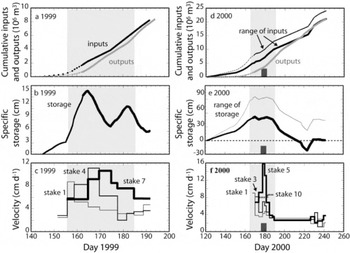
Fig. 11. Cumulative inputs and outputs (a, d), storage (b, e) and velocity (c, f) in 1999 and 2000, respectively. (a, d) Cumulative inputs (black line) were calculated using ablation stake data. In 2000 (d), we show two end-member calculations of water inputs, assuming either maximum early-season melt (thin black line) or zero storage by day 245 (thick black line). Outputs are the integrated water discharge record measured at the gauging station (gray). (b, e) Specific storage (inputs minus outputs divided by glacier area). For 2000 (e), we show the range of water-storage histories based on the possible range of cumulative water inputs. Water-storage peaks in the glacier ~day 165 in 1999 and ~day 170 in 2000, stays relatively high for ~20 days, and then decreases over the remainder of the melt season. Light gray boxes encompass the time during which elevated velocities were measured. The dark gray boxes (d, e, f) show the period of apparent bed separation measured at stake 5 in 2000.
Outputs
In both years, cumulative water outputs were calculated by integrating water discharge over the melt season. In 1999, water discharge prior to the installation of the stream gauge was estimated twice daily using the surface flow velocity and the width and depth of the flow; discharge varied between 0.01 and 1m3s-1. In 2000, the daily average discharge was >2m3s-1 upon our arrival in mid-June. We assume the total daily discharge increased smoothly from 0.1 to 2.3 m3s-1 between day 122 (laser altimetry data collection) and day 196 (stream gauge installation).
Inputs
To convert local melt rate into glacier-wide volumetric inputs, we assume that each ablation stake is representative of the melt rate in a surrounding area. We multiply the inputs by a constant ratio (drainage-basin area/glacierized- basin area) to account for melt in the portion of the drainage basin that is not glacierized. We assume the precipitation measured at the meteorological station is representative of the basin-averaged rainfall record, and use this record to incorporate rainfall into the basin water balance. Basal melt is ignored in our construction of cumulative water inputs, because we expect basal melt rates from geothermal and frictional heating to be insignificant (6-12 mm a-1; Reference PatersonPaterson, 1994, p. 112) relative to the meltwater production rate at the surface (1-4 m a-1).
In 1999, we assume that surface melt was negligible before the initiation of ablation-stake monitoring on day 149. This probably underestimates the total inputs of water into the basin, and therefore minimizes our calculation of storage. In 2000, we began measuring melt on day 165, although laser altimetry data and water-discharge rates suggest that melting had begun prior to the initiation of our field campaign. We allow volumetric water inputs to increase smoothly between days 122 and 165. Our estimate of 5 × 10⁶ m3 of meltwater before day 165 was set by assuming that the integrated inputs equal the integrated outputs by day 245, the last day of the 2000 field season. Assuming measurements of surface-elevation change between day 122 (laser altimetry) and day 165 are correct, snow density across the glacier would have been ~-330kgm-3 to accommodate this volumetric loss. This value is quite reasonable for late-winter/early-spring snow densities (e.g. Reference PatersonPaterson, 1994, p. 9). Alternatively, we can assume that the snowpack had already achieved a density of 520 kg m-3 by day 122 (when we measured it), in which case the total volume of inputs by day 165 is closer to 8 × 10⁶ m3 (thinner line in Fig. 11d).
There are several significant sources of error that are difficult to quantify for calculations of water input and output uncertainty. Potential water input uncertainties include changes in snowpack density (addition or loss of water within the snowpack over the summer), spatial variability in snowpack density, spatial variability in rainfall, variability in surface melt between stakes, spatial and temporal variation in snowmelt from the supraglacial part of the basin, and large spatial gaps between measurements in the accumulation zone. Uncertainties in water input may be ±20-50%. Water output uncertainties are related to errors in our rating curve, undocumented changes in the rating curve over time and possible subsurface transport of water. We estimate these uncertainties are closer to ±10% (Reference RiihimakiRiihimaki, 2003).
Specific water storage (inputs minus outputs divided by glacier area) increased through the early part of the melt season in both summers (Fig. 11b and d). Maximum water storage occurred on approximately the same calendar day (~days 165-170) in both years, although the estimated volume of water storage was three to six times greater in 2000. In both years, water storage remained high for approximately 20-25 days after storage peaked, and then declined for the remainder of the record. While the difference in total volume of storage in 1999 and 2000 is startling, it is important to note that S0 is unconstrained, creating significant uncertainty in the total volumes in both years.
Water storage in 1999 increased between days 145 and 164 as inputs exceeded outputs. The maximum water storage within the glacier reached 1.05 × 10⁶m3 (specific storage ~14cm) on day 165, and began decreasing immediately thereafter. Storage rose again between days 175 and 182, but then decreased for the duration of the measurement period.
In 2000, specific water storage reached a maximum of 50-85 cm sometime between days 165 and 170;the timing is dependent on the assumed Q i, Q o and S 0 before our arrival. Water storage fluctuated close to this maximum value until day 188, after which storage decreased steadily. On ~day 215, water storage dipped close to or below zero and was lowest on day 223. By day 230, water inputs and outputs closely track each other. In 2000, the lowest storage (~day 223) occurs immediately after a period of high water discharge, >7m3s-1. Negative values of water storage around day 220 suggest (1) we overestimated water discharge, (2) we underestimated melt in some portion of the basin during this time or (3) storage was already positive when measurements began (i.e. S 0 > 0). Adjusting for these effects would simply increase the total volume of water storage over the earlier portion of the melt season, putting the true storage maximum somewhere between our two end-member calculations. The use of point measurements to calculate areal melt, the lack of strong controls on melt in the non-glacierized portion of the basin and the low measurement frequency of ablation stakes 8-14 translate into a large uncertainty in our calculation of hydrological inputs to the basin. The need to estimate water discharge before our arrival at the glacier, and errors in discharge measurements account for uncertainty in water outputs from the basin. While uncertainties in volumetric water storage are high, we emphasize that the timing of the storage pattern is nonetheless a robust feature of the calculations.
The maximum volumes of water stored within the glacier translate into layers of water 14 and 50-85 cm thick over the glacier footprint for 1999 and 2000, respectively. At the time of maximum storage, water is likely stored in the snow/firn aquifer, in the englacial system of macro-pores and in cavities at the bed (Reference Fountain and WalderFountain and Walder, 1998).
Discussion
Relationship between sliding and water storage
Initiation of the propagating speed-up event occurs a few days before the storage peak in both 1999 and 2000 (Fig. 11). Migration of the zone of high basal motion occurs while storage is decreasing, but while it is still relatively high. In 1999, high velocities tail off around day 190, as water storage drops below 0.4 × 10⁶m3 (the equivalent of ~5 cm water across the glacier bed). In 2000, the zone of high sliding is within 1.5 km of the glacier headwall on day 185, when storage in the glacier begins to drop dramatically. In both summers, the water storage in the glacier continued to be positive after the propagating speedup event terminated in the accumulation zone. The speedup event is initiated either during times of high rates of increase in total water storage (1999), or close to the time of greatest water storage (2000). Interestingly, the maximum volume of water stored in the glacier is >3.5 times greater in 2000. It is possible that S 0 was greater in 1999 (i.e. significant melt had occurred prior to our arrival and prior to the speed-up event, or was retained from the previous summer), and that a ‘critical melt volume’ is required for initiation of rapid sliding; however, field evidence to constrain this volume of melt is lacking.
High vertical velocities were also measured during the time of increased water storage in 2000 (Figs 10 and 11f). Apparent bed separation at stake 5 occurred between days 176 and 182, which corresponds with a time of relatively high water storage. Water storage in the glacier was slightly increasing between days 175 and 182, the time of highest vertical and horizontal velocities at stake 5. The glacier surface was again moving roughly parallel to the bed slope by day 190, 2000, and no additional bed separation events occurred during the melt season. However, water storage was not fully depleted until a large discharge event ~day 220. In both years, increasing water storage coincided with increased basal motion (and uplift of the surface in 2000), while decreasing water storage was not reflected in either the vertical or the horizontal velocity records after the propagating speed-up event.
Some studies of glacier surface velocity suggest that speed-up events throughout the melt season are associated with warmer temperatures and/or increased melting across the glacier (e.g. Reference Iken, Rothlisberger, Flotron and HaeberliIken and others, 1983; Reference Iken and TrufferIken and Truffer, 1997). From our work and additional measurements made in 2002 (Reference AndersonAnderson and others, 2004), it appears that only low (2-3 cm d-1) and roughly steady melt rates are needed to induce an early melt season high-velocity event at Bench Glacier. Importantly, increases in temperature and associated peaks in surface melting rate later in the season fail to trigger increased basal motion. For example, the temperature increase ~days 220-230 in 2000 is associated with increased melting (Fig. 9b), but is not accompanied by any increase in measured surface velocity. However, we note that only one extreme rainfall event occurred during the two-summer study (~day 260, 1999), and limited data suggest there may have been an increase in surface velocities in the ablation zone during that time. The fact that the propagating speed-up event occurred early in both summers, and that no additional high-velocity events were recorded, suggests the glacier not only can transmit more water but also can accommodate greater input variability later in the melt season without triggering enhanced basal motion.
Basal boundary conditions
Our observations of divergence and convergence of the ice surface with the bed associated with rapidly changing horizontal velocity are similar to observations made on Unteraargletscher, Switzerland (Reference Iken, Rothlisberger, Flotron and HaeberliIken and others, 1983, Fig. 2). Superimposed on an extended period of uplift are short-term uplift events, each very similar to the single uplift event documented at Bench Glacier. Reference Iken, Rothlisberger, Flotron and HaeberliIken and others (1983) infer that the long-term uplift implies long-term hydrological storage, while the short-term speed-up and uplift event suggests a rapid change, or transition, in the state of basal cavity development. They infer that early in the melt season, water pressure in small and poorly connected basal cavities increases quickly in response to increased water inputs. This should encourage basal motion, which both increases the size of the cavities and promotes connections among them. This process should increase both the overall capacity and the efficiency of the hydrologic system.
It is likely that the propagating speed-up event measured at Bench Glacier reflects a change in the basal boundary conditions. The observed sliding at individual stakes is consistent with a typical spring event documented on other glaciers as a result of either elevated water pressure or water storage (e.g. Reference Iken, Rothlisberger, Flotron and HaeberliIken and others, 1983; Reference Iken and BindschadlerIken and Bindschadler, 1986; Reference Hooke, Calla, Holmlund, Nilsson and StroevenHooke and others, 1989; Reference Harper, Humphrey and GreenwoodHarper and others, 2002). High water pressures are thought to increase sliding speed both because they increase separation of the ice from the bed (Reference LliboutryLliboutry, 1979; Reference Iken, Rothlisberger, Flotron and HaeberliIken and others, 1983), thereby reducing the bed friction, and because they exert a down- glacier force on down-glacier basal cavity walls (Reference IkenIken, 1981). Thus, the propagating speed-up event probably occurred in response to increased water pressure due to continuing meltwater input to an englacial and then subglacial system that was hydraulically inefficient at moving water about. The detailed records of melt across Bench Glacier suggest that, while the velocity events are not triggered by an increase in melt rate, they may initiate once a threshold volume of melt has occurred. In 1999, rapid basal motion was initiated after only ~10-20 cm of melt had occurred at the terminus, although we emphasize that our measurements of melt began only 1 week prior to the initiation of the speed-up. In 2000, laser altimetry data suggest ~1 m of melt had occurred at the terminus at the time of speed-up initiation. Interestingly, data from 2002 show that the propagating speed-up event also initiated after 1 m of melt had been generated at the terminus (Reference AndersonAnderson and others, 2004). It is therefore possible that a volumetric trigger for enhanced basal motion does exist; this in turn would correspond to a threshold of water pressure and hence effective pressure, as discussed by, for example, Reference Iken and TrufferIken and Truffer (1997) and Reference AndersonAnderson and others (2004).
Alternative mechanisms for the uplift event
Based on the relationship between horizontal velocity, surface uplift and water storage, and the similarities between our observations and those at other glaciers, we infer that the observed surface uplift reflects basal motion along up- glacier inclined bedrock steps at Bench Glacier. Here we discuss and reject two other possible causes for surface uplift: local ice thickening due to longitudinal strain of the ice and shearing of subglacial sediments.
Local ice thickening
Gradients in the horizontal velocity field could cause thickening of the glacier, resulting in an increase in the elevation of the local ice surface. The maximum offset may be calculated by assuming continuity and incompressibility:
where w is vertical velocity, w
s the vertical velocity at the surface, ![]() the horizontal strain rate averaged over the vertical ice profile, and H is ice thickness. For ice ~185 m thick, a vertical velocity of ~3cmd-1 requires
the horizontal strain rate averaged over the vertical ice profile, and H is ice thickness. For ice ~185 m thick, a vertical velocity of ~3cmd-1 requires ![]() to be on the order of 17 cmd-1 km-1. Importantly, while stake 5 was moving at 15 cm d-1, rapid motion (~ 14-15 cm d-1) was also occurring at stakes 6C and 4, which are ~1 km apart on either side of stake 5. The initiation of rapid motion appears to have begun simultaneously at all three stakes; i.e.
to be on the order of 17 cmd-1 km-1. Importantly, while stake 5 was moving at 15 cm d-1, rapid motion (~ 14-15 cm d-1) was also occurring at stakes 6C and 4, which are ~1 km apart on either side of stake 5. The initiation of rapid motion appears to have begun simultaneously at all three stakes; i.e. ![]() over this portion of the ablation zone. It is therefore unlikely that a gradient in horizontal velocities could be responsible for local ice thickening and apparent surface uplift.
over this portion of the ablation zone. It is therefore unlikely that a gradient in horizontal velocities could be responsible for local ice thickening and apparent surface uplift.
Observations of transverse cracking of the snow support our conclusion that compression is not responsible for surface uplift. In both years we observed transverse cracks in the snow surface across the full glacier width, perpendicular to the ice-flow direction, during propagation of the speed-up event. In 1999, cracks occurred between stakes 2C and 3 on day 157, when stakes 1 and 2C were moving more rapidly than stake 3, which had yet to reach its peak velocity (Fig. 3a). Cracks were subsequently observed further up- glacier over the next 15 days. In 2000, surface cracks occurred between stakes 5 and 6C on day 171, when the velocity event was peaking at stake 3 and had not yet reached further up-glacier. Observations of cracks suggest that extension, rather than compression, dominates in the longtitudinal direction. In this case ![]() and w
s <0 is predicted. Based on these observations consistent with extensional flow, our calculations of bed separation are minima, as ice strain would predict surface lowering.
and w
s <0 is predicted. Based on these observations consistent with extensional flow, our calculations of bed separation are minima, as ice strain would predict surface lowering.
Limited velocity data from cross-glacier stake lines 2A-2E and 6A-6E do not show measurable divergence from parallel, down-glacier flow, suggesting transverse strain rates do not vary significantly over the summer. Because we have no data on vertical strain rates, it is not possible to consider the role of variability in vertical strain in the observed propagating speed-up events.
Shearing of subglacial sediments
Reference Iken, Rothlisberger, Flotron and HaeberliIken and others (1983) discuss the possible role of shearing and subsequent volume change of subglacial sediments in causing glacier surface uplift. Following their arguments, we calculate >4m of till would be required to produce the observed uplift; this value is an order of magnitude greater than likely till thickness at Bench Glacier (Reference MacGregorMacGregor, 2002). It is yet more difficult to explain the rapid convergence of the ice surface with the bed subsequent to termination of sliding. Given the likely very low hydraulic diffusivity of subglacial sediment, deflation of a dilated till would be likely to take much longer than the 5 day timescale observed.
Conceptual model
The up-glacier propagating speed-up event reflects the glaciological response to the early-melt-season evolution of the hydrological system. During the winter months, motion at Bench Glacier appears to be dominated by internal deformation. Water discharge from the glacier is minimal, and it is likely that there is very little change in water storage within the glacier over the winter. In the absence of water flow in the subglacial system, any large conduits that may exist at the end of the last melt season will close, except for those under very thin ice near the terminus. The rate of tunnel closure is ~1 cm d-1 under 100 m thick ice, and ~9cmd-1 under 200 m thick ice (Reference PatersonPaterson, 1994, p. 115, equation 7). Tunnels with a 2 m radius (the approximate size of the conduit at the terminus) would therefore close under all but the terminal region of Bench Glacier over the winter.
The propagating speed-up event at Bench Glacier coincides with the maximum water storage in the late spring/early summer. We suggest that the consistent pattern of basal motion observed illuminates the gross spatial and temporal distribution of water pressures, and hence effective stress, at the bed. Higher melt rates, lower ice thickness and thinner snowpack should all promote enhanced basal motion first near the terminus. Low effective stresses must occur over an area of the bed that is likely to be on the same scale as the coupling length of a temperate glacier, of the order of many ice thicknesses (Reference Echelmeyer and KambEchelmeyer and Kamb, 1986; Reference Kamb and EchelmeyerKamb and Echelmeyer, 1986). That the Bench Glacier sliding motion appears to be smoothed on such length scales is reflected in the coherence of the sliding pattern (Fig. 3). High water pressures have been measured by another team at points and over small areas of the glacier that have not been associated with enhanced basal motion (Reference Harper, Humphrey and PfefferHarper and others, 2003), this may reflect measurement over too small an area to have captured the relevant mean pressure.
Rapid basal motion locally increases the sizes of the cavities and the connections between them, and hence enhances the hydraulic connectivity of the cavity system. Movement of water between cavities and into existing conduits near the terminus will cause frictional melting, promoting further linkage between cavities in the area of rapid sliding. The conduit, in turn, will extend up-glacier, driven by the high head gradients between the adjacent linked-cavity system and the conduit. Water from the more connected conduit system exits the glacier more rapidly than through the winter cavity-dominated system. Drainage of water from cavities will ultimately lower the effective water table in the englacial system, reducing the pressures in the enlarged cavities at the bed, thereby reducing local sliding. Rapid sliding also increases the size of basal cavities as long as the system remains sufficiently pressurized to prevent cavity collapse. This allows transfer of water from storage in the englacial system into storage at the bed; it therefore lowers the water pressures by dropping the effective water table. We note that this does not alter the storage as measured by the mismatch of inputs and outputs from the glacier. Both of these effects, the loss of englacial and subglacial water through the conduit system, and the transfer of water from englacial storage to enlarged cavities at the bed, serve as brakes on glacier sliding.
High vertical velocities during the most rapid horizontal motion support the idea that the glacier is sliding up the stoss slopes of a set of bedrock bumps. The drop in the horizontal sliding rate at the termination of the speed-up event reflects a reduced local pressure, which results from loss of water from the linked-cavity system to a lengthening conduit. The simultaneous initiation of rapid lowering of the ice surface suggests that basal cavities then begin to collapse as water pressure is lowered. Within a week after termination of the propagating speed-up event, surface motion asymptotically approaches mean bed-parallel. Subsequent, slower basal motion must then be dominated by regelation.
After passage of a conduit tip past a site, water will move through the linked-cavity network toward the low-pressure conduit, lowering the pressure head in the linked-cavity system rapidly at first and more slowly with time. That the storage of water within the glacier declines monotonically after the termination of the speed-up event (Fig. 11) reflects the long time-scale (20-30 days in 2000) over which water stored within the linked-cavity network and the englacial system above it continues to migrate to the conduit system. This long time-scale may reflect either a low degree of interconnectedness within the remaining cavity system, isolation of the conduit from cavities or both. That sliding at a site terminates well before this storage is exhausted supports the notion that there is a sliding threshold, requiring local water storage and associated pressures above a critical level.
As surface melt rates increase and the snowpack thins over the middle of the summer, the subglacial hydrologic system must accommodate increasing magnitude and variability of melt input rates. That this increased meltwater input fails to trigger further rapid basal motion reflects the higher capacity of the now conduit-bled subglacial hydrologic system once the propagating speed-up event has passed, which prevents subsequent pressurization of the subglacial system. The late-season growth in maximum daily discharge, and the reduction in the lag between meltwater inputs and stream discharge, reflect both the existence of an efficient conduit system, and the progressive loss of a snow aquifer as the snowline translates up-glacier.
Conclusions
Observations of surface motion and water balance on Bench Glacier reveal a consistent pattern that implicates seasonal evolution of the subglacial hydrologic system. The early season up-glacier propagating speed-up event can be explained by the pressurization of a poorly connected subglacial linked-cavity system, while its termination can be explained by an increase in efficiency of the subglacial hydrologic system through the up-glacier insertion of a conduit. As the event begins, melt input exceeds water output over most of the glacier. As it terminates, more area of the glacier is losing water through the conduit system at a rate that exceeds the melt input rate. Glacier-wide storage of water therefore peaks in the midst of the sliding event.
The detailed vertical and horizontal records at one stake, documented using static DGPS, suggest that the rapid motion of the speed-up occurs through essentially block sliding up the stoss sides of bedrock bumps. The opening of cavities and their subsequent collapse upon termination of the sliding at this site inspired a more extensive deployment of GPS monuments in 2002, which reveal a similarly rich record of motion (Reference AndersonAnderson and others, 2004). Finally, the record of sediment discharge from the glacier can be used to explore the degree to which seasonal variation in sediment output reflects the annual sliding history (Reference RiihimakiRiihimaki, 2003).
Acknowledgements
This work was supported by a grant from the US National Science Foundation (NSF) (OPP98-18251), a NASA Earth Systems Science Graduate Fellowship (to K.R.M.) and an NSF Graduate Fellowship (to C.A.R.). We thank J. Harper, P. Adams, G. Stock, K. Lawrence, C. Pollack and R. Helms for help in the field. We gratefully acknowledge ERA Helicopters and VECO Polar Resources for field support and UNAVCO for GPS equipment. We thank I. Willis and R. LeB. Hooke for editorial comments on the manuscript, A. Fountain for editorial comments and K. Cuffey for assistance as the Scientific Editor. This is Center for the Study of Imaging and Dynamics of the Earth submission No. 447.


