


Introduction
The knowledge of snow surface characteristics of ice sheets is important for many reasons. The snowpack is the interface between the atmosphere and the underlying ice, controlling the exchange of energy and mass (Reference Brun, Martin, Simon, Gendre and ColéouBrun and others, 1989, Reference Brun, David, Sudul and Brunot1992). The albedo of snow depends on the snow effective grain-size and the surface characteristics (Reference Grenfell, Warren and MullenGrenfell and others, 1994; Reference Marshall and OglesbyMarshall and Oglesby, 1994; Reference WintherWinther, 1994; Reference Fily, Leroux, Lenoble, Sergent, Schmitt, Bergh and FestouFily and others, 1998). The snow is the initial stage of the densification and trapping of air in the firn and the ice (Reference Alley and BentleyAlley and Bentley, 1988; Reference Arnaud, Lipenkov, Barnola, Gay and DuvalArnaud and others, 1998), and finally the snow physical characteristics control the remote-sensing measurements (Reference AlleyAlley, 1987; Reference BindschadlerBindschadler, 1998; Reference Fily, Leroux, Lenoble, Sergent, Schmitt, Bergh and FestouFily and others, 1998, Reference Fily, Dedieu and Durand1999; Reference Genthon, Fily and MartinGenthon and others, 2001).
Most physical properties of snow and ice cover are clearly defined and measurable except for the grain geometry which can be difficult to characterize (Reference ColbeckColbeck and others, 1990; Reference ColbeckColbeck 1991). A simple method suitable for field measurements of grain-size is to place a sample of snow grains on a ruled plate. The average size is then estimated by comparing the mean size of the grains with the marks on the plate. The definition of size is not unique for three-dimensional non-isotropic objects. One common definition of grain-size is the greatest extension of the grains (Reference ColbeckColbeck and others, 1990) measured in millimeters or classified from “very fine” (<0.2 mm) to “very coarse” (2.0–5.0 mm). For the purpose of reflectance modelling, Reference Grenfell, Warren and MullenGrenfell and others (1994) used the same technique to measure the smallest, rather than the greatest, extension, which is generally closer to the diameter of an equivalent sphere with the same surface/volume ratio. An approximate distribution of grain-sizes may also be obtained by snow sieving or by automated image-processing techniques. Many other definitions of grain-size can be found (Reference AlleyAlley, 1987) and this must be taken into account when comparing measurements reported by different authors.
Our goal in this paper is to propose an objective method to determine one well-defined snow grain-size parameter. Because the method is objective and reproducible, measurements made at different places and times by different operators are quantitatively comparable. The method is based on the analysis of digital images of snow grains. First, in a technical section, we describe the image-acquisition techniques and the numerical algorithm to determine grain-size from the images. Then, in a results section, data obtained from a large number of samples and images collected in different places in Antarctica are presented and discussed (Fig. 1). The samples were collected as part of national or international Antarctic scientific traverses (e.g. Reference Winther and WintherWinther and others, 1997). The spatial and depth coverage of the current archive is still very limited. It is expected to progressively develop into a comprehensive dataset of snow images and grain-sizes as new exploratory traverses (e.g. as part of International Trans-Antarctic Scientific Expeditions (ITASE); Reference Mayewski and GoodwinMayewski and Goodwin, 1999) bring more high-quality data.
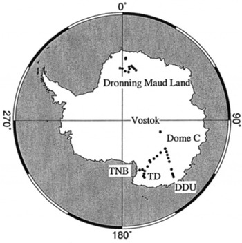
Fig. 1. Antarctic map showing location of sampling sites. TNB, Terra Nova Bay; DDU, Dumont d’Urville; TD, Talos Dome.
Image-Acquisition Techniques
Slices of high-density firn can be cut, and thick sections have been produced with microtome before an image of the surface is taken (Reference Arnaud, Lipenkov, Barnola, Gay and DuvalArnaud and others, 1998). The process cannot be applied to lower-density snow in the upper meters of the snowpack, unless cohesion is increased by impregnation before slicing (Reference AlleyAlley, 1980; Good, 1989). This is technically too difficult and too labour-intensive to be implemented in situ on a regular basis. We have tested three lighter techniques to acquire digital images of snow grains.
Technique 1: Snow samples are collected in small flasks filled with isooctane (trimethyl 2-2-4-pentane) to prevent metamorphism after collection (Reference Brun and PahautBrun and Pahaut, 1991). The samples are then kept at temperatures well below freezing and transported to the Laboratoire de Glaciologie et Géophysique de l’Environnement (LGGE) where digital images are taken in a cold laboratory. For this, a binocular microscope is used with a mounted digital camera linked to a computer. After drying on filter paper, snow grains and clusters are separated (using a toothpick-like tool) on a glass window and illuminated from below (transmitted light). The magnifying factor depends on the mean grain-size. It is chosen to be between 2 and 3, so that three to four grains or clusters are captured on each image (Fig. 2a). Technique 1 (Reference Lesaffre, Pougatch and MartinLesaffre and others, 1998) was used at all sites for which results are presented in section 3. Additionally, other methods were tested at some of the sampling sites.

Fig. 2. (a) Digital image of snow grains collected in the field and transported in isooctane (technique 1) with scale in 1/10 mm.(b) Photograph of snow grains acquired in situ (technique 3) at the same site (itb8 at 1.5 m depth) along the Terra Nova Bay–Dome C traverse with scale in mm.
Technique 2: Classic (film) macrophotographies of snow grains are taken in the field and then digitized at LGGE (Fig. 2b). A 50 mm macro-lens and an additional ring set the magnifying factor to 2. In this case, the grains are dispersed on a dark plate and the illumination is diffuse from above (reflected light). As the film definition is very good, a second enlargement can be obtained when digitizing the slides. Technique 2 was used along a Terra Nova Bay–Dome Concordia (Dome C) traverse (Fig. 1).
Technique 3: Digital images were acquired in the field when adequate facilities were available. This was done at Dome C (Fig. 1) where a digital camera was available in a cold laboratory close to the sampling site. Because of the material resources needed, technique 3 may be used at a fixed point but generally not on traverses.
About 50 different grains (i.e. about 15 images, each showing 3–4 grains) of each snow sample were analyzed to obtain a statistically significant measure of the mean size. Dispersal and separation of grains for each image, a rather delicate and time-consuming operation, may be hard to accomplish in the field. On the other hand, taking photographs directly in the field (techniques 2 and 3) may be safer than sampling in isooctane flasks for imagery back in the laboratory (technique 1). Indeed, over the past few years, a number of snow samples have been lost due to insufficiently cold conditions during transport. Our results prove that all of the three above techniques yield good results and may be recommended, depending on the logistical and technical support available in the field and for the transport phase.
Digital image processing
Perfect separation of snow grains for imagery is generally difficult and barely fully realized. Clustering of snow grains is a major problem, which prevents the use of stereologic quantities based on the area or the lengths of the objects to determine grain-sizes. To avoid biases associated with grain clustering, a size parameter is defined only from the contour of the snow grains or clusters: it is the mean radius of all the convex parts of the ice/air boundaries, or the mean convex radius. This parameter was found to be representative of the grain-size for metamorphism (Reference Lesaffre, Pougatch and MartinLesaffre and others, 1998). For example, it is the size parameter, along with dendricity and sphericity, used in the snow-metamorphism model Crocus (Reference Brun, David, Sudul and BrunotBrun and others, 1992). The mean convex radius was also found to be the best grain-size parameter for modelling of snow reflectance in the near-wave infrared spectral domain (Reference Fily, Bourdelles, Dedieu and SergentFily and others, 1997, Reference Fily, Dedieu and Durand1999; Reference Sergent, Leroux, Pougatch and GuiradoSergent and others, 1998).
For mean convex radius measurement, the contour of the object needs to be digitally identified from an original grey-scale image. This is done by transforming the grey image into a binary (black and white) image, a process called image segmentation.
Image segmentation
For each pixel P(x, y) of an image, the local gradient G(x, y) is obtained from the surrounding pixels using a Sobel operator over a 3 × 3 region:
with

where the z’s are the grey levels of the pixels, z 5 corresponding to pixel P(x, y) (Table 1).
Table 1. Grey-level indices used for the Sobel operator

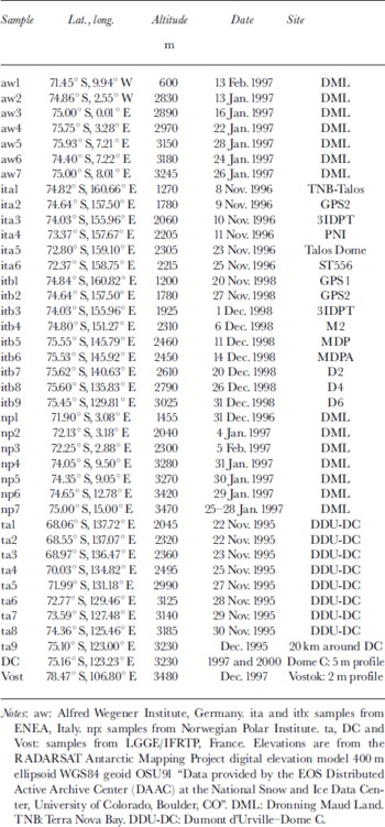
Once the procedure is completed for all possible pixels, the result is a gradient image of the same size as the original image (Fig. 3a). The lines of highest gradients, above a minimum threshold (Fig. 3b), define discrete contours. Each object is then defined as the set of connected pixels whose gradient value is less than this minimum threshold. The image “background" is given the value 1, and all the objects (the grains) the value 0. The result is a binary image with each object being a grain or a cluster of grains (Fig. 3c).
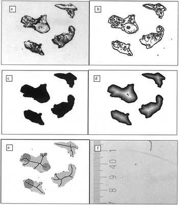
Fig. 3. (a) Original image of a few snow grains; (b) gradient image; (c) binary image; (d) distance map; (e) skeleton and examples of maximal disks contained in the snow grains; (f) scale in 1/10 mm.
Mean convex radius
The mean convex radius may simply be computed as the mean radius of curvature of the curves locally fitting the discrete contour where it is convex (Reference Lesaffre, Pougatch and MartinLesaffre and others, 1998). The accuracy of this method depends on the number N of contour pixels used to fit the discrete contour, and errors can be as high as 30%. In order to reduce the error, N must be optimized depending on the size of the grains on the digital image. Therefore, as N is kept constant, it is necessary to adapt the magnifying factor to the grain-size, which is not possible when there is a large range of grain-sizes on the same image. To overcome this problem, we use an alternate method based on the skeletization of each object (grain) on an image. This method is more robust and can provide various size parameters depending on the final application.
The weighted skeleton is a reduced but complete representation of an object. The construction of a skeleton (Reference Sanniti di Baja and ThielSanniti di Baja and Thiel, 1996) requires determination of the distance between each object pixel and the object boundary. Consider a digital binary image, consisting of object and non-object pixels (Fig. 3c). We use a distance transformation which is an operation that converts this binary image to a grey-level image, where each object pixel has a value corresponding to the distance to the nearest contour pixel (Fig. 3d). The new image is called a distance map and can be interpreted as the result of a propagation process: a wave front originating from the object contour propagates at uniform speed towards the inside. This is described in detail in Reference Sanniti di Baja and ThielSannitti di Baja and Thiel (1996). In particular, we use the chamfer distance transformation on a 5 × 5 pixel neighborhood (Reference BorgeforsBorgefors, 1986; Reference ThielThiel, 1994; Reference Sanniti di Baja and ThielSanniti di Baja and Thiel, 1996) as a practical proxy for Euclidean distance. The difference with actual Euclidean distance is, in this case, then < 2%.
From the distance map the skeleton is found. If we consider the distance map as a topographic map, with the highest pixels associated to the largest distances, the skeleton can be simply defined as the ridges of this topographic surface. For a two-dimensional digital image it is defined as the locus of centers of maximal disks contained in the object (Fig. 3e). A skeleton is composed of branches with nodal points at their intersections and end-points at their extremities.
A maximal disk, and therefore a radius, contained in the object can be associated to each pixel of the discrete skeleton (Reference Chassery and MontanvertChassery and Montanvert, 1991). In particular, one radius is associated to each end-point of the skeleton which is representative of the convexity of the contour close to it (Fig. 3e). The mean convex radius is the average of all these radii. The radii associated to nodal points of the skeleton are more representative of the volume of the grains, or clusters of grains. The weighted skeleton could also provide information on the shape of the grain (Reference Chassery and MontanvertChassery and Montanvert, 1991), but this is beyond the scope of this paper.
Results
Comparison of sampling and image-analysis techniques
Images of more than 500 snow samples were collected for different locations and depths in Antarctica, thanks to the activity of French, German, Italian and Norwegian field parties in recent years (Table 2; Fig. 1). Sampling technique 1 (isooctane flasks) was systematically used at all sites and along all traverses. Techniques 2 or 3 (imagery on the field) were also used at Dome C and along the Terra Nova Bay– Dome C traverse. All images (about 3000 altogether) were processed with the same image-analysis method for grain-size determination, as described above. The equivalence of the different sampling techniques can thus be assessed.
Table 2. Sampling locations and dates
All the results are given in Figures 4–6. To allow a simple visual comparison of the grain-sizes, the same scale, but not the same range, is used for all the sites. The error bars represent the standard deviation of all the mean convex radii obtained for one sample.

Fig. 4. Mean convex radius of snow grains vs depth at Dome C and Vostok. The error bars represent one standard deviation of all the measurements obtained for one sample. The dots (●) are from digital images of snow samples collected in the field in 1997 and transported to Grenoble in cold isooctane (technique 1). The squares (□) are from digital images acquired at Dome C in 2000 (technique 3).

Fig. 5. Mean convex radius of snow grains vs depth along the Terra Nova Bay–Dome C traverse (Table 2; Fig. 1). The dots (●) are from digital images of snow samples collected in the field in 1997 and transported to Grenoble in cold isooctane (technique 1). The triangles (△) are from classical photos acquired in situ (technique 2).

At Dome C (Fig. 4) the sizes obtained from isooctane samples (technique 1) and from digital images (technique 3) acquired 2 years later are very similar. This demonstrates (1) that snow metamorphism in cold isooctane during transportation and storage in good conditions is negligible, and (2) that the same results are obtained when different techniques are applied by different operators at different times. This is further confirmed by Figure 5, which compares grain-sizes along a Terra Nova Bay–Dome C traverse as obtained from photographs taken in the field (technique 2) and from snow samples brought back to LGGE (technique 1). Photographs visibly showing massive clustering and insufficient separation of grains were discarded. In most cases, results from both techniques are very similar. Large differences may be found in some places because the samples were not taken in exactly the same layer and because the grains were too clustered.
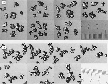
From the same weighted skeleton, different size parameters can be computed. The radii computed from end-points and nodal points are compared for many sites (Fig. 6). Examples of digital images of snow grains are given for the two sites aw2 and aw6 in Figure 7. When the grains are well separated and easily identified (Fig. 7a; aw6 at 0.4 m) the two size parameters are similar (∼0.15 mm). When the grains are clustered (Fig. 7b; aw2 at 0.2 m), the nodal radius (∼0.5 mm) is larger than the end-point radius (0.1mm) because it is more sensitive to the volume of the object than to the shape of its contour. As clustering of snow grains is difficult to avoid, we prefer to use the mean convex radius as defined from the skeleton end-points. This also emphasizes the importance of the definition of the size parameter when different samples are compared.
Spatial and depth variations of Antarctic snow grain-size
The results obtained from the 42 sites in Antarctica tend to show that near the surface (0–0.5 m) the mean convex radius is surprisingly spatially homogeneous, of the order of 0.1–0.2 mm almost everywhere. They may be classified as very fine to fine grain (<0.2 to 0.5 mm) according to Reference ColbeckColbeck and others (1990). Comparison with other in situ data reported in the literature is difficult because the size was determined visually and therefore it does not represent the same parameter.
The largest variability is found along the Terra Nova Bay–Dome C traverse (Figs 5 and 6). The sizes obtained from samples acquired at a 2 year interval are very similar for 31DPT (samples ita3 and itb3) and different for GPS2 (samples ita2 and itb2). GPS2 is a site with erosional forms up to 15 cm and seasonal wind crust, whereas 31DPT site presents depositional forms about 10 cm and has more homogeneous snow stratigraphy than GPS2. Larger grain-sizes are found at M2 (itb4) and MDP (itb5) sites even at the surface. This is in agreement with older traverse data (Reference Stuart and HeineStuart and Heine, 1961) and could explain the peculiar microwave signature observed there (Reference Surdyk and FilySurdyk and Fily, 1993). These sites are characterized by wind crust, consisting of a single snow-grain layer cemented by thin (0.1–2 mm) films of sublimated ice. Under strongly developed wind crust the depth-hoar layer clearly indicates prolonged sublimation due to a hiatus in accumulation and therefore a long, multi-annual, steep temperature-gradient metamorphism (Reference GowGow, 1965). Either the large grain or the wind crust (Reference Wiesmann, Fierz and MätzlerWiesmann and others, 2000) could explain the peculiar microwave signature observed (Reference Surdyk and FilySurdyk and Fily, 1993). Sites MDP (itb5) and MDPA (itb6) are only at a distance of 5 km, and show quite different grain-size profiles, both for mean values and for variability. MDPA site shows sastrugi up to 20 cm high but no permanent wind crust. The large difference in grain-size between the two sites is due to the different snow-redistribution process at local scale. Reference Frezzotti, Gandolfi, La Marca and UrbiniFrezzotti and others (2002) point out that along the Terra Nova–Dome C traverse, wind crusts are present in a wide area of the plateau, and are strictly correlated with snow-redistribution process due to downwind slope >0.25° (0.4% or 4 m km−1).
At Vostok and Dome C, more variations in grain-size occur below 1 m, and a significant difference is found between the two sites. At Vostok, there is a sharp increase in grain-size between 0.6 and 0.8 m depth. The evolution of size is smoother at Dome C. The size is almost identical between 2 and 5 m as observed in situ.
All sites where the variations of size with depth are significantly sampled show a broad increase with depth. This is expected, as metamorphism tends to favor the growth of the larger grains with time, at the expense of the smaller grains. The rate of increase with depth is not uniform. At Dome C and Vostok, grain-size remains fine in the upper few tens of cm (1 m at Dome C, 50 cm at Vostok), whereas grains are larger at or near the surface at itb4 and itb5. A simple age/depth relationship suggests that accumulation is lower at the latter sites. There is little increase in grain-size at itb4 and itb5 below 50 cm.
Conclusion
Size parameters automatically obtained from digital images of snow grains allowed comparisons between samples acquired by different people at different locations in Antarctica. Similar results were obtained with various acquisition techniques (classical photos or digital camera) that can be used during any scientific expedition with minimum equipment and facilities. One of the most difficult problems is the separation of snow grains, which is solved by choosing a size parameter based on the contour of the objects, the mean convex radius, and a robust image-analysis technique based on skeletization of the objects.
Data from 42 sites in Antarctica were analyzed. For radiative balance (albedo), only the surface grains must be considered, so no large variations due to grain-size are expected in those areas, except between Terra Nova Bay and Dome C. For metamorphism studies, the profiles obtained down to 2 m depth and even better down to 5 m at Dome C could be used with the available density profiles to validate and improve snow-metamorphism model results (Reference Dang, Genthon and MartinDang and others, 1997; Reference Genthon, Fily and MartinGenthon and others, 2001).
The database which has been initiated will be increased in order to obtain a map of grain-size variations of the Antarctic ice sheet. This will improve understanding of the snow metamorphism in Antarctica in relation to climatic parameters.
Acknowledgements
This research was carried out within the framework of the European Community project Polar Snow (Contract ENV4-GT95-0076), the SPOT4/Vegetation Preparatory Program (96/CNES/0394), a Project on Glaciology and Paleoclimatology of the Programma Nazionale di Ricerche in Antartide (PNRA), and was financially supported by Ente per le Nuove Tecnologie, l’Energia e l’Ambiente (ENEA) through a cooperation agreement with the Universit degli Studi di Milano. This work is a contribution of the Italian branch of the ITASE project. The authors wish to thank all members of the traverse teams, and the institutes which were in charge of the logistics: Institut Français de Recherche et Technologie Polaire (IFRTP), France; ENEA, Italy; Alfred Wegener Institute for Polar and Marine Research, Germany; Norwegian Polar Institute. A. Hubert (South Through the Pole Expedition) made a vital contribution to the design and tests of field photographic equipment.


