


Notation
1. Introduction
More than one-fifth of the global population relies on glacier- and snowmelt for water resources (Reference Immerzeel, Van Beek and BierkensImmerzeel and others, 2010), and glacier meltwater plays a pivotal role in water supply for downstream regions (Reference Immerzeel, Van Beek and BierkensImmerzeel and others, 2010; Reference Pellicciotti, Buergi, Immerzeel, Konz and ShresthaPellicciotti and others, 2012; Reference Prasch, Mauser and WeberPrasch and others, 2013). Snowfall and glaciers are among the most susceptible land surfaces affected by climate change. Glacier retreat and its impact on runoff due to climate change have attracted wide public attention. As glacier and snow retreat continues or even accelerates, additional fresh water is expected to be released from glacier storage, altering the hydrological processes, freshwater supply and water cycle (Reference XuXu and others, 2009; Reference Immerzeel, Van Beek and BierkensImmerzeel and others, 2010; Reference Kang, Xu, You, Flügel, Pepin and YaoKang and others, 2010; Reference YaoYao and others, 2012). Therefore, estimation of runoff from glacierized basins has been a key issue in water resource management in alpine regions (Reference ViviroliViviroli and others, 2011).
The Tibetan Plateau (TP) (sometimes referred to as the ‘Third Pole’) contains abundant glaciers (Reference YaoYao, 2008). Over recent decades, most TP glaciers have shrunk (Reference BolchBolch and others, 2012; Reference YaoYao and others, 2012; Reference Gardelle, Berthier and ArnaudGardelle and others, 2013; Reference GardnerGardner and others, 2013; Reference Molg, Maussion and SchererMolg and others, 2013; Reference Neckel, Kropáček, Bolch and HochschildNeckel and others, 2014). Glacier shrinkage in the Himalaya and the inner TP will pose serious problems for water resources (Reference KehrwaldKehrwald and others, 2008; Reference KangKang and others, 2015), and play an important role in river water discharge (Reference Immerzeel, Van Beek and BierkensImmerzeel and others, 2010). Recent studies have also found that glacier melt is the most likely cause of the recent increases in lake level (G. Reference Zhang, Wu, Zhu, Wang, Li and ChenZhang and others, 2011). In alpine regions, especially in the TP, available meteorological data are scarce. There have been few or no hydrometeorological observations in the vast area of high-altitude mountainous regions with sparse human activity. To understand hydrological processes and the response of glacier runoff to climate change, in order to guide water management, it is necessary to use hydrological models that simulate snow and glacier processes. Recent studies of the influence of glacier melt on river runoff have been mainly based on different catchments, large- or small-scale (Reference Rees and CollinsRees and Collins, 2006; Reference Immerzeel, Van Beek and BierkensImmerzeel and other, 2010, Reference Immerzeel, Van Beek, Konz, Shresta and Bierkens2012). Reference HussHuss (2011) used glacier mass balance to calculate meltwater release in Europe. Reference Sorg, Bolch, Stoffel, Solomina and BenistonSorg and others (2012) showed that glacier shrinkage in the Tien Shan was most pronounced in peripheral, lower-elevation ranges near the densely populated forelands, where summers are dry and where snow and glacial meltwater is essential for water availability. Reference Ding, Yang and ChenDing and others (2013) developed an energy-balance-based glacier melt model which could reasonably simulate the glacier melting process for the TP. The contribution of glacier- and snowmelt to rivers in the TP ranged from 5% to 45% of average flow (Reference Xu, Gong and LiuXu and others, 2007). The coupled modeling approach with regional climate model outputs and a process-oriented glacier and hydrological model showed that in a central Himalayan river basin, ice melt from glaciers is and will be a minor component of runoff in the summer-monsoon-dominated Himalayan basin due to the small fraction of the glacier area in the whole basin (Reference Prasch, Mauser and WeberPrasch and others, 2013). Due to different glacier states (shrinking, advancing or stable) and precipitation patterns on the TP (e.g. Reference YaoYao and others, 2012; Reference Kapnick, Delworth, Ashfaq, Malyshev and MillyKapnick and others, 2014; Reference Song, Huang, Richards, Ke and PhanSong and others, 2014), detailed studies of glacier melt, its relation to precipitation and temperature, and the meltwater contribution to river water are needed to address the future role of snow/glaciers for downstream water resources (Reference Immerzeel, Van Beek and BierkensImmerzeel and others, 2010; Reference Prasch, Mauser and WeberPrasch and others, 2013).
To model spatially distributed hydrological processes, a modular object-oriented framework system, JAMS/J2K, has been developed to simulate hydrological processes in river basins, and extended by incorporating a WaSiM-ETH temperature index method (Reference HockHock, 1999; Reference Schulla and JasperSchulla and Jasper, 2007; Reference Gao, Kang, Krause, Cuo and NepalGao and others, 2012). In a previous study, the JAMS/ J2K model was used to simulate and calibrate the discharge of the Qugaqie basin based on data only from the downstream hydrological station (Reference Gao, Kang, Krause, Cuo and NepalGao and others, 2012). The results showed that the simulated discharge was generally less than the observed values for the calibration and validation periods. Hypothetical climate scenario experiments showed that an increase in air temperature by 1°C resulted in a 14% increase in runoff, whereas a 20% increase in precipitation caused a 9% increase in runoff but a 12% reduction in glacier melt. The energy-balance model of Zhadang glacier indicated that the specific mass balance was more sensitive to change in precipitation than to other variables (Reference ZhangZhang and others, 2013). Based on the J2K model, the observed Nam Co lake level rise was reproduced and runoff from glacierized areas appeared to be the most important contributor to lake level increase (Reference Krause, Biskop, Helmschrot, Flugel, Kang and GaoKrause and others, 2010). However, B. Reference Zhang, Wu, Zhu, Wang, Li and ChenZhang and others (2011) also maintained that the Nam Co lake water storage increase was closely related to increasing precipitation, with less impact from glacier meltwater (Reference Zhou, Kang, Chen and JoswiakZhou and others, 2013). In this study, we applied the distributed hydrological model JAMS/ J2K in the Qugaqie basin and the Zhadang sub-basin located in the southern TP to investigate the effects of climate change on glacier mass balance and runoff. The hydrological data used in the model expanded to two stations located upstream and downstream of the Qugaqie basin. In the study, we modeled the snowmelt from glacier surfaces based on the concept of linear reservoirs; in addition, variable combinations of three temperature-index snowmelt models and two glacier melt models, which were integrated into JAMS/J2K, were used to calculate snow- and ice melt. A multi-object optimization method, MOCOM, developed by Reference Yapo, Gupta and SorooshianYapo and others (1998), was used to calibrate the model’s physical and conceptual parameters with reference to four model error metrics. To specifically account for the role of glacier melt in the Qugaqie basin, we calculated the contribution of glacier meltwater to river runoff not only for the highly glacierized Zhadang sub-basin, which is the headwater of Qugaqie, but also for the downstream area. After evaluating the simulated glacier melt runoff, the runoff variations in Qugaqie basin and Zhadang sub-basin were investigated under the climate change scenarios.
2. Study Area
The Nyainqêntanglha mountain range is located in the southern TP within a transition zone from maritime glaciers in southeast Tibet to continental glaciers in the north. Nam Co basin is located along the northern slope of Nyainqêntanglha mountain (Fig. S1 in Supplementary Material (available online at http://www.igsoc.org/hyperlink/14j170_supp.pdf)). As one of the main contributors to Nam Co lake, glacier melt runoff is of great importance to the hydrological processes and water balance in the basin.
Nam Co basin, with an average altitude >4700 m a.s.l., consists of various landforms (rivers, lakes, glaciers, permafrost, wet land, alpine meadow, etc.) and serves as a natural Earth-science laboratory (Fig. S2 (http://www.igsoc.org/hyperlink/14j170_supp.pdf)). A multidisciplinary observation and research station (30°46.44′ N, 90°59.31′ E; 4730 m a.s.l.) was established in the Nam Co lake basin in summer 2005, and has been maintained by the Institute of Tibetan Plateau Research, Chinese Academy of Sciences (Fig. S1 (http://www.igsoc.org/hyperlink/14j170_supp.pdf)). The establishment of the Nam Co station makes it possible to monitor the hydrometeorological and cryospheric conditions in the lake basin.
The Qugaqie basin is located on the northern slope of Nyainqêntanglha with an area of 59 km2, formed by two tributaries that converge upstream of the Qugaqie head (Fig. 1). The largest headwater sub-basin (6 km2, 34% of the glacierized area), the Zhadang basin, is located in the southeastern portion of the Qugaqie basin and is predominantly upland in character, with an altitude ranging from 4760 to 6090 m (Fig. 1). More detailed information can be found in Reference Gao, Kang, Krause, Cuo and NepalGao and others (2012). Zhadang glacier (5Z225D0017, 30°28.57′ N, 90°38.71′ E) is located on the northern slope of Nyainqêntanglha (Fig. 1), covering an area of 2.0 km2 and having a length of 2.2 km (Reference ZhangZhang and others, 2013). Zhadang glacier is a valley-type glacier facing north-northwest with an elevation range of 5515–6090 m a.s.l. It has a fan-shaped terminus without debris cover (Reference KangKang and others, 2009). Two automatic weather stations (AWSs) are installed at 5400 and 5800 m a.s.l. on the glacier (Reference Gao, Kang, Krause, Cuo and NepalGao and others, 2012; Reference ZhangZhang and others, 2013). The glacier mass balance has been observed since the Nam Co station was established in September 2005 (Reference KangKang and others, 2009; Reference ZhangZhang and others, 2013). A large deficit in summer resulted in negative annual mass balances of ∼1200 mm during 2005–12 (Reference QuQu and others, 2014).
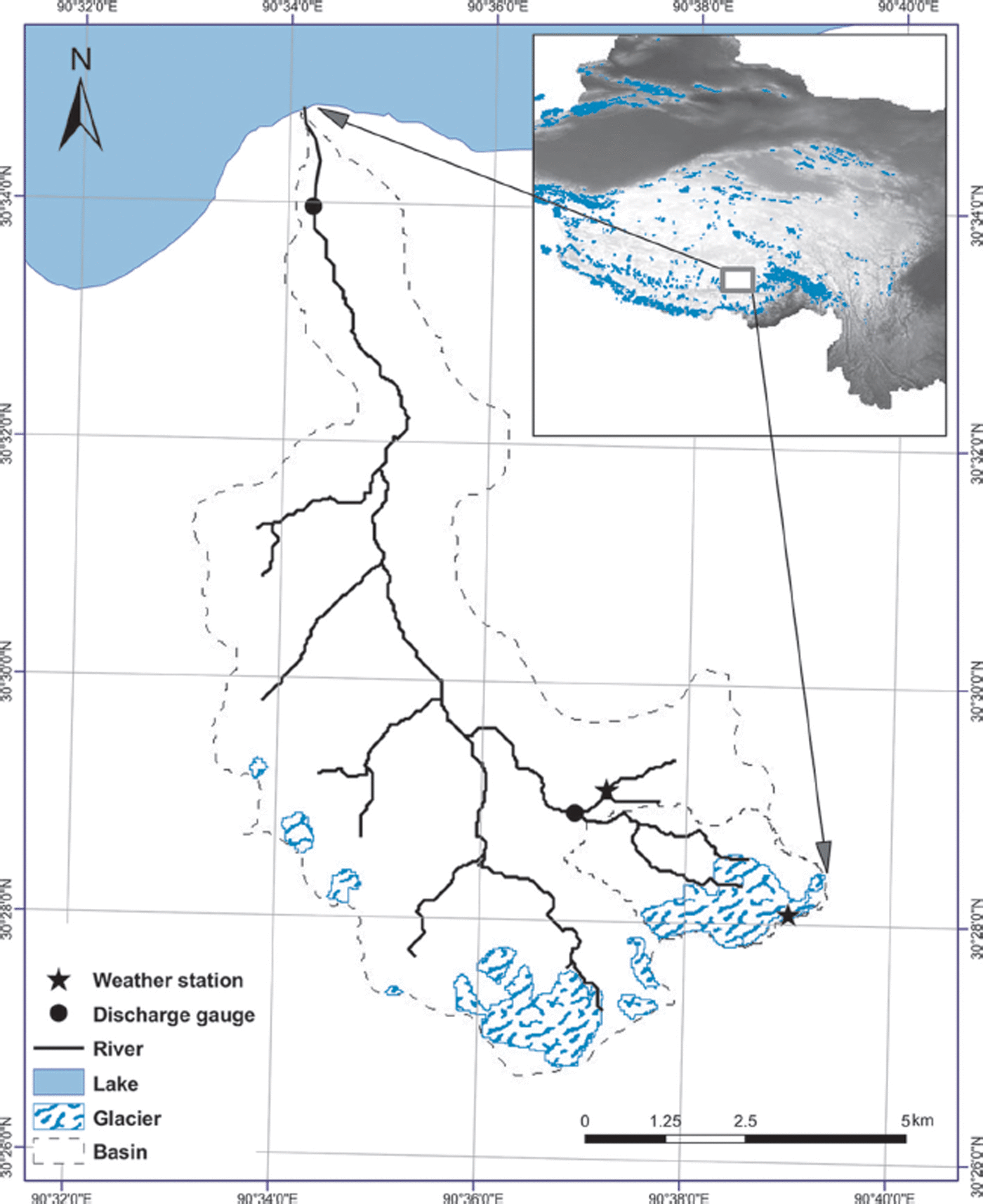
Fig. 1. Location map of the Qugaqie basin in the Nam Co basin, Tibetan Plateau (detailed information in Supplementary Material (http://www.igsoc.org/hyperlink/14j170_supp.pdf)).
3. JAMS/J2K Model System
The JAMS/J2K model was developed within the modular oriented framework JAMS (Jena Adaptable Modelling System) which is a spatially distributed hydrological model with a minimum number of parameters for calibration and is capable of conducting data pre- and post-processing, analyzing sensitivity and uncertainty, and plotting diagrams of the model results (Reference KrauseKrause, 2002; Reference Kralisch, Krause, Fink, Fischer and FlugelKralisch and others, 2007; Reference Gao, Kang, Krause, Cuo and NepalGao and others, 2012). The JAMS/J2K requires spatially distributed information on topography, land use, soil type and hydrogeology to estimate specific attribute values for each modelling unit (Reference Krause, Biskop, Helmschrot, Flugel, Kang and GaoKrause and others, 2010). It is forced by temperature, precipitation and wind speed. JAMS/J2K originated from the gridded hydrological model WaSiM-ETH (Reference Schulla and JasperSchulla and Jasper, 2007). In this study, combinations of two glacier-melting methods (G1 and G2) and three snowmelting methods (S1, S2 and S3) were incorporated in JAMS/J2K to simulate glacier runoff.
3.1. Hydrological response units
The spatial discretization of JAMS/J2K relied on the hydrological response unit (HRU). HRUs are areas that consist of homogeneous land use, climate and underlying pedo-topogeological properties controlling hydrological dynamics (Reference FlügelFlügel, 1995). They are delineated by overlying layers of elevation, slope, aspect, land use, soil type and sub-basin mask using ESRI ArcGIS®. The HRU-specific spatial information was stored in a table and loaded into J2K during model initialization. Figure S3 (http://www.igsoc.org/hyperlink/14j170_supp.pdf) illustrates the response units of the Qugaqie basin (including the Zhadang basin), which was divided into 1269 HRUs. To simulate the detailed spatial variations in glacier melting, a 30 m × 30 m grid rather than HRU division was used for the glacial areas in the Zhadang basin, and the runoff from each gridcell flowed directly into the stream channel.
3.2. Data preparation
3.2.1. DEM data
The digital elevation model (DEM) data were 30 m × 30 m resolution, obtained from the Advanced Spaceborne Thermal Emission and Reflection Radiometer (ASTER) Global DEM (GDEM), available from the World Science Academy Computer Network Information Center (http://datamirror.csdb.cn). Other model input data (e.g. basin perimeter, slope, aspect) were generated using the hydrological analysis module in the ArcGIS software. The ArcGIS processes included filling sinks, generating terrain slopes and aspects, flow direction, flow accumulation, water level, etc. The base map used in the ArcGIS process was the DEM.
3.2.2. Land-cover/-use data
Land-cover/-use data with 100 m × 100 m resolution were provided by the Data Sharing Infrastructure of Earth System Science and were obtained based on the 1:1000 000 national land-use data and classification of remote-sensing data, originally from the national ecosystem map (http:// www.geodata.cn).
3.2.3. Soil data
Soil data were collected from 1 : 10 000 000 digitized soil maps from the Soil Database of the Institute of Soil Science, Chinese Academy of Sciences (http://www.soil.csdb.cn/), and were divided into 12 soil classes and 61 soil types using the traditional Soil Genetic Classification System. The soil type of each land cover/use was calculated according to the United States Department of Agriculture (USDA) Soil Triangle. The physical and chemical properties of each soil layer were obtained by matching to the soil texture in each layer.
3.3. Regionalization of climate data
Due to the sparsity of meteorological observations in the TP, model forcings were obtained from three weather stations in the Qugaqie basin and the adjacent area. One was Nam Co station, 45 km from the Qugaqie basin, and the other two were AWSs installed at the pass (5800 m a.s.l.) on Zhadang glacier and off-glacier (5400 m a.s.l.) near the terminus area (Fig. 1). Meteorological data included temperature, wind speed, relative humidity and solar radiation. In the J2K model, the meteorological data are interpolated in both the vertical (e.g. decreasing temperature with increasing elevation) and horizontal (e.g. horizontal variability of rainfall) directions for each time step (Reference KrauseKrause, 2002; Reference Gao, Kang, Krause, Cuo and NepalGao and others, 2012). The daily lapse rate of the temperature value, which fluctuates from day to day and was calculated from he observation data, is used in the vertical direction, while the reversed distance weighting method was used in the horizontal direction.
Precipitation amounts were observed and recorded at Nam Co station and Zhadang sub-basin. Nam Co station used a manual observation method, recording at 08:00 and 20:00 local time every day. The rain gauge near the glacier terminus AWS was an RG3-M tilting precipitation recorder with a resolution of 0.2 mm. RG3-M can only be used in the summer as it cannot accurately measure snow. To eliminate systematically biased errors in the precipitation measurements due to the wind speed, type and frequency of precipitation, etc., the regionalization methods were improved by incorporating precipitation under catch correction functions developed by Reference Yang, Shi, Kang, Zhang and YangYang and others (1991) and Reference Ye, Yang, Ding, Han and KoikeYe and others (2004). The calibrated summer precipitation was increased at ∼14.4% in the Qugaqie basin.
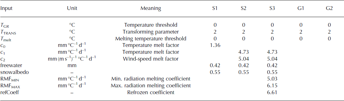
To measure snow accumulation, the model divides precipitation into rainfall and snowfall according to temperature. If the temperature in the HRU is lower than the temperature threshold parameter (T GR: 0°C), the precipitation is recorded as solid, otherwise it is recorded as liquid. A transforming parameter (T TRANS: 2) is used to determine the temperature range when most precipitation is snow or rain (Reference Ye, Yang, Ding, Han and KoikeYe and others, 2004). Table 1 lists the parameter values used in the model.
Table 1. Data requirements and calibrated parameters of the snowmelt modules
4. Glacier/Snow Accumulation and Melting Models
Six algorithms developed by combinations of two glacier-melting methods (G1 and G2), and three snowmelting methods (S1–S3) were used to simulate glacier runoff.
4.1. S1 (temperature index)
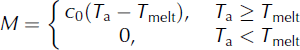
The temperature-melting method was based on the basic degree-day factor, which only uses interpolated temperature to drive the simulation in the HRUs. When daily temperature in the HRUs was below the threshold temperature for melt (T melt), glacier ablation was set to zero; when it was greater than the threshold, the ablation was calculated from
4.2. S2 (temperature–wind index)
The temperature–wind index approach considers both temperature and wind-speed impacts on snowmelt. Spatially interpolated temperature and wind speed drives the simulation in the HRUs. If the daily temperature in the HRUs is below the melt threshold, the ablation is zero, while if it is above the threshold
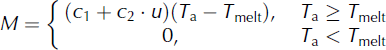
4.3. S3 (combined Anderson and Braun approach)
The Reference AndersonAnderson (1973) and Reference BraunBraun (1985) methods consider the refreezing process of snowmelt when the temperature falls below the melt threshold (T melt). Parameter c 1 is defined as the temperature melting factor (Table 1). The effective snow ablation is the proportion of rain- and snowmelt exceeding c 1. If the temperature is below the melt threshold and the water stored in the model experiences a refreezing process, then
In the calculation of the accumulation and ablation for refrozen snow and ice, the forcings were spatially interpolated precipitation, temperature and wind speed. When the daily temperature (T a) in the HRU is above the temperature threshold (T melt), the melt is calculated as
It is assumed that the glacier starts to melt when there is no snow cover. In this study, two methods were applied to calculate glacier melt: the temperature index method (G1), and the improved temperature index method developed by Reference HockHock (1999, Reference Hock2005) which uses information on global radiation (G2).
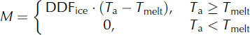
4.4. G1 (temperature index method)
Glacier ablation was determined by the temperature and degree-day factor. The range of the degree-day factor for glacier melt was 10–15 mm °C−1 d−1 for Zhadang glacier (Reference Wu, Kang, Gao and ZhangWu and others, 2010).
4.5. G2 (temperature–radiation method)
The temperature–radiation method took into account the global radiation. The melt was determined by the temperature, radiation and glacier melt empirical coefficient:
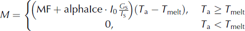
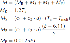
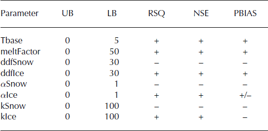
The JAMES/J2K model contained two glacier melt equations and eight parameters (Table 2), the tbase, meltFactor, ddfSnow, ddfIce, alphaSnow, alphaIce, kIce and kSnow.
Table 2. Parameter boundaries (lower boundary: LB; upper boundary: UB) and sensitivity (+: high; −: low) of each parameter for the three objective functions: coefficient of determination (RSQ), Nash–Sutcliffe efficiency (NSE) and percent bias (PBIAS)
5. Sensitive Parameter Identification and Model Optimization
5.1. Parameter sensitivity analysis
Parameter sensitivity analysis can improve the understanding of model structures and model processes, reducing the number of parameters for calibration. In addition, it may help identify the effects of individual parameters and the interactions among the parameters on the simulation, which decreases the model’s uncertainty (Reference SchmidtSchmidt, 2000). Multi-parameter sensitivity analysis (also called generalized sensitivity analysis) can determine the influences of a number of parameters contemporaneously. In the JAMS/J2K model, feasible parameter ranges and parameter distributions within these ranges have to be defined prior to the analysis. Then a Monte Carlo analysis is used to produce a large number of different parameter combinations and to obtain a model response for each of them (Reference Wagener and KollatWagener and Kollat, 2007). In this study, the analysis was an extension of the regional sensitivity analysis (RSA); the general idea was to split the various model samples into good (behavioral) and bad (non-behavioral) populations and compare their distribution functions in the parameter/objective function space (Reference Freer, Beven and AbroiseFreer and others, 1996).
The approach first ranked the objective function and paired the ranked objective function with corresponding parameter values. The paired values were separated into ten equal-numbered bins. In each bin, the cumulative distribution of the ranked objective function was calculated, then the distribution was plotted against the parameter values. The spread of the cumulative distributions illustrated the parameter sensitivity. A wider spread depicted higher sensitivity of the parameter.
The 3000 values of the model parameters were randomly sampled within the parameter ranges shown in Table 2, and the model was run 3000 times with the corresponding parameter values. The objective functions used in the sensitivity analysis were the Nash–Sutcliffe coefficient (NSE), relative bias (PBIAS) and correlation coefficient between the simulated and observed runoff (RSQ), which were compared with the baseline scenario (hand calibration) to obtain the sensitivity results. Table 2 also shows the sensitivity result of each parameter compared with NSE, PBIAS and RSQ. The results show that the ddfSnow, alphaSnow and kSnow parameters for the three objective functions are relatively insensitive, while the others are relatively sensitive.
Figure 2 shows the cumulative distributions of the objective functions vs the parameter values. The tbase and alphaIce are moderately spread; hence, they are of medium sensitivity. The meltFactor, ddfIce and kIce parameters have a large spread, indicating high sensitivity in the glacier module. The ddfSnow, alphaSnow and kSnow appear to be the least sensitive parameters. The parameter sensitivity generally shows a consistent pattern among the three model metrics, although PBIAS shows a smaller spread in the cumulative distributions.
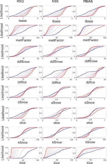
Fig. 2. The regional sensitivity analysis of the glacier module based on RSQ, NSE and PBIAS (x-axis represents the different parameter set, y-axis the likelihood, red coarse line the best group and blue coarse line the worst group).
The sensitivity of runoff to parameter changes in the J2K model was examined by NSE (Fig. 3). The glacier runoff parameters (ddfIce, ddfSnow, kIce and kSnow) were the most sensitive, followed by the surface runoff parameters (cOFactor, tbase, meltTemp and flowRouteTA). The underground runoff parameters (e.g. initRG, gwRG and gwCapRise) were the least sensitive. The results indicated that groundwater in the Qugaqie basin contributes little to the streams in the basin, whereas summer glacial melt and surface runoff dominated the streamflow. The observation also implied that the contribution from snow was much smaller than the contribution from the glaciers to the streams. The results also indicated that the soil infiltration, snowmelt and snow storage constant had low sensitivity or even non-sensitivity, consistent with the fact that the Nam Co basin is located in the monsoonal region and the precipitation is mainly concentrated in summer (∼90%; see Fig. S4 (http://www.igsoc.org/hyperlink/14j170_supp.pdf)) (Reference KangKang, 2011). During the melt season, the snow albedo (snowConstAlbedo in Fig. 3) also had low sensitivity. This may be due to the thin snow on the glacier during the melt season keeping albedo at a consistently low level and thus playing a minor role in runoff variability.
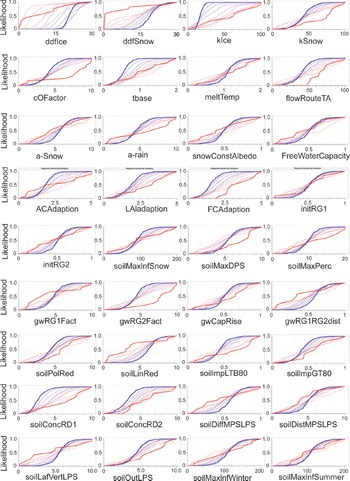
Fig. 3. The RSA of the J2K model based on the NSE (x-axis represents the different parameter set, y-axis the likelihood, red coarse line the best group and blue coarse line the worst group).
5.2. Parameter optimization
We utilized the Multi-Object COMplex evolution (MOCOM-UA) algorithm, an effective and efficient methodology for solving the multiple-objective global optimization problem (Reference Yapo, Gupta and SorooshianYapo and others, 1998), to calibrate various combinations of the snow and ice modules. MOCOM-UA, based on the SCE-UA population evolution method (Reference Duan, Sorooshian and GuptaDuan and others, 1992), involved the initial selection of a population of P points distributed randomly throughout the s-dimensional feasible parameter space. A detailed description and explanation of the methods is provided by Reference Yapo, Gupta and SorooshianYapo and others (1998).
The calibration period for the Qugaqie basin was 2006–07, while it was 2007 for the Zhadang sub-basin. The validation period was 2008. Due to the harsh environmental conditions in the TP during winter, there was a lack of observations during winter for the frozen river water. Five objective functions were chosen to examine the goodness-of-fit between the simulations and observations during optimization: (1) the minimum annual average runoff deviation (PBIAS); (2) the maximum NSE; (3) the maximum correlation coefficient between the simulated and the observed runoff (RSQ); (4) the minimum root-mean-square error (RMSE); and (5) the maximum logarithm function of Nash–Sutcliffe (LNSE). These functions are calculated:
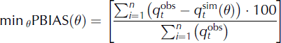
where PBIAS is the deviation of data being evaluated, expressed as a percentage;
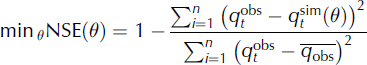
where NSE indicates how well the plot of the observed versus simulated data fits the 1 : 1 line;
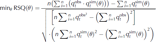
where RSQ describes the degree of collinearity between the simulated and measured data;
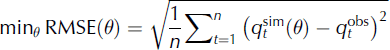
where RMSE estimates the residual variance between the measured and simulated values; and
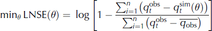
where LNSE describes the logarithm of NSE.
The five objective functions tend to provide different parameter estimates, resulting in different simulated hydrographs. The multi-objective problem is defined as
The calibration and validation results for various combinations of the ice/snow modules in the Qugaqie basin and Zhadang sub-basin are shown in Table 3. The optimum values of RMSE, NSE and RSQ in the Zhadang sub-basin during calibration are obtained from the combinations G2 + S2 and G2 + S3. The best results for PBIAS were from the combinations G1 + S2 and G1 + S3. During validation, the optimum values of RMSE and RSQ were from the combination G2 + S3, the best NSE was from the combinations G2 + S2 and G2 + S3, and the optimum PBIAS was from the combination G2 + S1. The calibration and validation results for the Qugaqie basin were similar to those for the Zhadang sub-basin. The calibration and validation showed that the glacier melt method G2 performed better than G1, while the best snowmelt method was S3, although the difference was small among the various snow modules. The optimization demonstrated that runoff in the Qugaqie basin was mainly influenced by glacier melt, while the impact of different snow modules on the runoff was small. Snowmelt played a pivotal role in the runoff and water balance in alpine regions. Its contribution to runoff was one of the important water resources in mountainous regions, in addition to rainfall and glacier melting (Reference Zhang, Xie, Yao, Liang and KangZhang and others, 2012). In Nam Co basin, there existed a more continuous snow cover before summer melting, and the majority of annual snow cover melted away in summer to supply more water to the lake (Kropacek and others, 2010; Reference Zhang, Xie, Yao, Liang and KangZhang and others, 2012). However, in the studied basin, due to the large glacier area, the contribution of snowmelt to the runoff was less than that of glacier melt.
Table 3. The calibration and validation under various ice/snow models
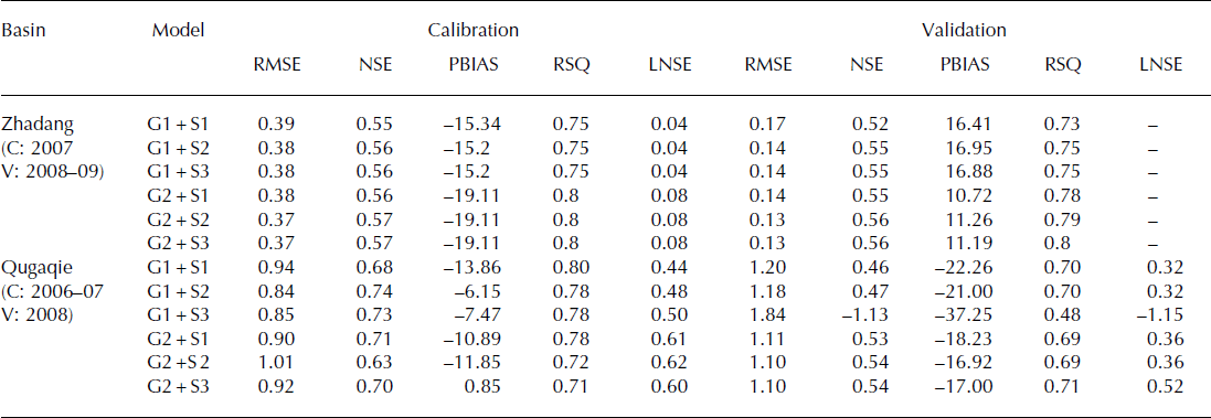
The calibration results in the Qugaqie basin were inferior to those in the Zhadang sub-basin, which may be because glacier runoff contributes more to the streamflow in the Zhadang sub-basin than in the Qugaqie basin. These results perhaps also show that the model needs improvement in simulating the hydrological processes in grasslands and bare lands. Nevertheless, the optimization showed that the J2K simulation results were reliable in both the Qugaqie basin and Zhadang sub-basin.
The calibration and validation of the glacier and snow modules (Table 3) showed that the G2 + S3 combination performed best in the Zhadang basin. The result of G2 + S2 was very similar to that of G2 + S3, though with slightly lower RMSE and PBIAS values. In addition, the best combination in the Qugaqie basin was G2 + S1, indicating that the revised glacier melt module G2 can account for the melting process in the whole Qugaqie basin. These results further demonstrate that the traditional temperature-index method, when considering the global radiation and glacier/ snow melt empirical coefficient, was better at simulating glacier runoff than the degree-day factor method.
Among the snowmelt modules, S3 and S2 were better than S1 when considering the snow’s thermal changes and refreezing processes. Figures 4 and 5 illustrate the runoff simulation using the optimized modules of G2 + S3. In the Qugaqie basin (Fig. 4), the simulated and observed runoff show similar variability, with most of the total runoff occurring in summer. The contribution of glacier melt to the runoff is ∼50%. In the Zhadang basin, the simulated runoff is close to the glacier melt. The observed runoff peaks in July and August of 2007 and 2009 and is much higher than the simulated runoff (Fig. 5). However, the simulated and the observed runoff in 2008 show only small variability, and the monthly total values are similar from May to September, reflecting small glacier melt contributions to the river flow (Reference KangKang and others, 2009). In August–October 2009 (Fig. 5), the glacier melt runoff is almost equal to the simulation, indicating that precipitation makes a small contribution to runoff. In addition, glacier surface albedo is enhanced in winter when snow covers the glacier (Reference Fujita, Ohta and AgetaFujita and others 2007).
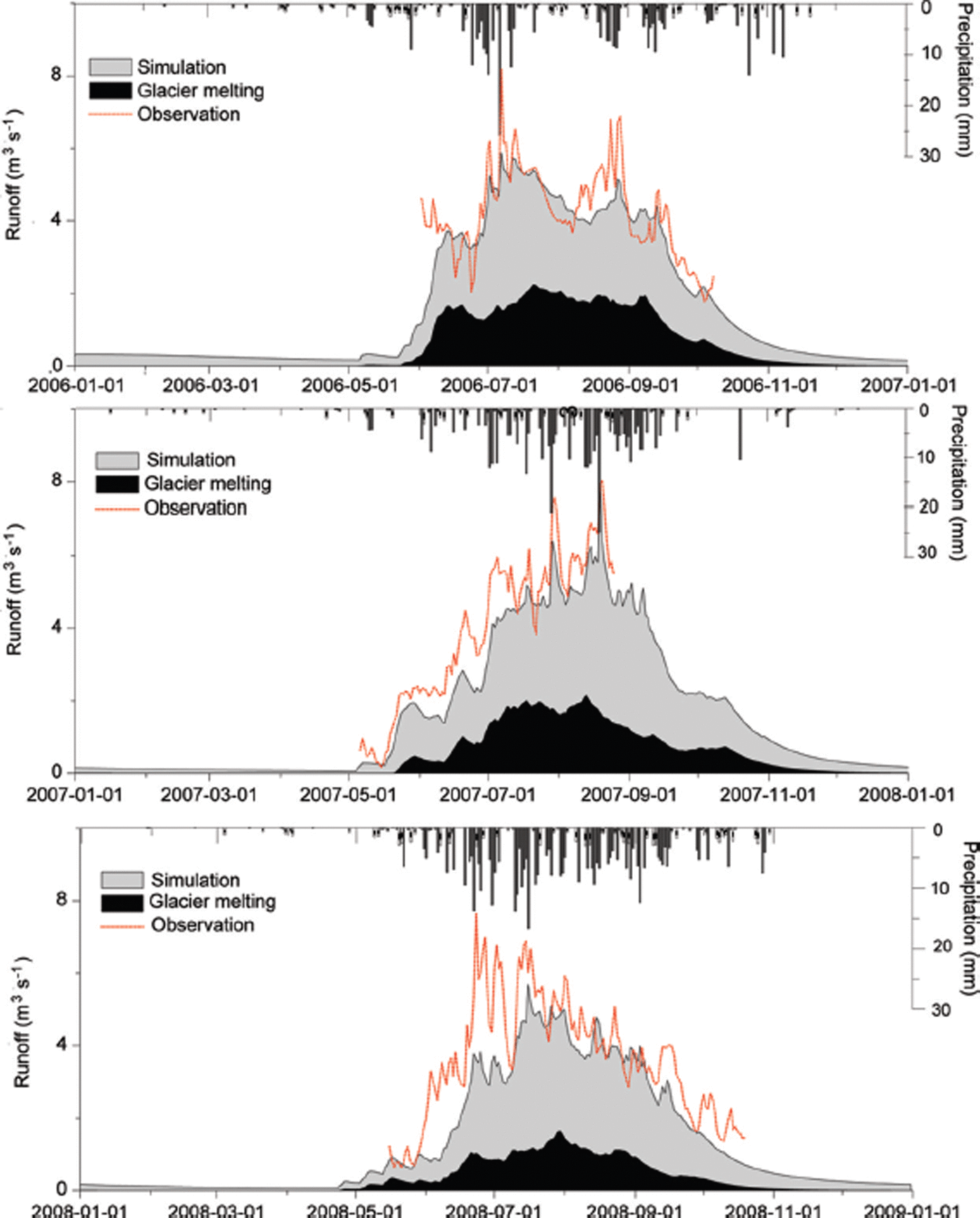
Fig. 4. Simulated and observed runoff from the Qugaqie basin after optimization (2006–08). Date format is yyyy-mm-dd.
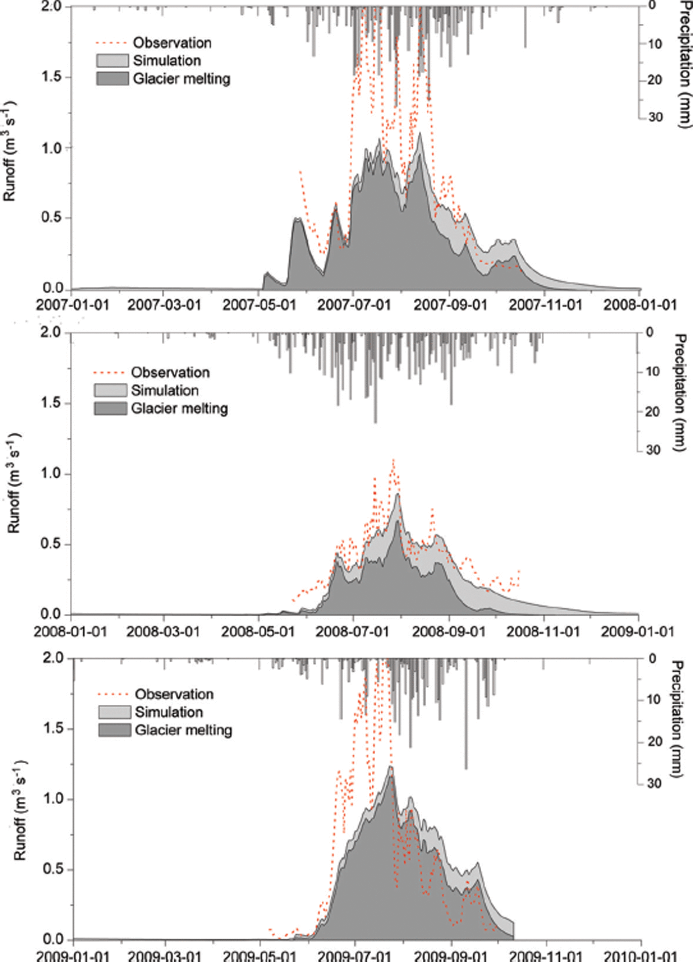
Fig. 5. Same as Figure 4, but for the Zhadang basin
6. Glacier Melt and Mass-Balance Simulation
Based on the G2 + S3 combination method, we simulated glacier melt and mass balance. During 2006–08, the simulated glacier melt runoff in the Qugaqie basin contributes 58%, 50% and 41% to the streamflow, respectively, with the highest monthly contributions occurring in June (65.6%) and July (65.3%). The glacier melt runoff in the Zhadang sub-basin during 2007 and 2008 contributes 78% and 66%, respectively, to the streamflow, with the highest contributions in June and July. Because of rising temperature, the glacier melt contribution is high in June and July, coinciding with the onset of monsoonal precipitation in the region.
The simulated and observed mass balance of Zhadang glacier in 2006/07, 2007/08 and 2008/09 are shown in Figure 6. The observed mass balances were −783, 223 and −1705 mm, respectively, and the simulated mass balances are −450, −214 and −1370 mm, respectively. Large negative mass balances occurred during the 2006/07 and 2008/09 observation periods, but a positive mass balance occurred in 2007/08 due to the early onset of the rainy season, which suppressed glacier melt (Reference KangKang and others, 2009). The simulated negative mass balances are higher than observed, explaining the underestimation of the glacier melt.
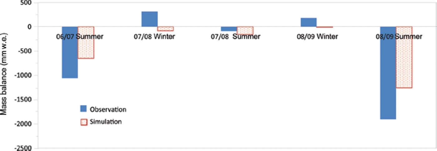
Fig. 6. Comparison of seasonal glacier mass balance for Zhadang glacier from observation and simulation. The observed mass-balance data are from Reference KangKang (2011) and Reference QuQu and others (2014).
Comparison between the simulated and observed Zhadang glacier mass balance during 2006–09 shows similar variability (R 2 = 0.85) (Fig. 7), indicating that the J2K model can accurately simulate the glacier mass balance, doing relatively well in the summer melt season. However, in the accumulation season, there is a discrepancy between simulations and observations. This may be because the precipitation data for the winter used in the model come from Nam Co station, which is ∼60 km from the Qugaqie basin. It is possible that the regional weather variation caused a spatial variation in the winter precipitation. In addition, based on the same method, Reference Fujita, Ohta and AgetaFujita and others (2007) found that the simulation results in winter, when the snow-covered glacier had high albedo, were much lower than observed. Surface albedo is a critical factor in glacier mass balance, and is dramatically affected by snow and ice surface conditions. Reference Fujita, Ohta and AgetaFujita and others (2007) found that changes in air temperature caused an increase in melting by sensible heat and reduced albedo, since some of the snowfall changes to rainfall. Snowfall in winter on the glacier surface resulted in high albedo, which effectively reduced the solar radiation absorption by the glacier, preventing glacier surface melt and hence reducing glacier runoff (Reference Verbunt, Gurtz, Jasper, Lang, Warmerdam and ZappaVerbunt and others, 2003; Reference Fujita, Ohta and AgetaFujita and others, 2007). In the melt season, however, precipitation form was variable and rainfall could occur due to high air temperature (Reference ZhangZhang and others, 2013), resulting in the albedo having less effect on the melt amount (Reference FujitaFujita, 2008). Reference Fujita, Ohta and AgetaFujita and others (2007) found that changes in both air temperature and precipitation strongly affected glacier runoff by changing the surface albedo during the melt season, although these perturbations only slightly altered the annual averages. Energy-balance analysis has shown that Zhadang glacier surface albedo is affected by variations in precipitation form, resulting in large interannual variability in glacier meltwater (Reference Zhou, Kang, Gao and ZhangZhou and others, 2010). The seasonal pattern of precipitation also significantly affected the climatic sensitivities of glacier balance (Reference FujitaFujita, 2008; Reference Kapnick, Delworth, Ashfaq, Malyshev and MillyKapnick and others, 2014). The latest study found that light-absorbing impurities (e.g. black carbon and dust on the glacier surface) play an important role in reducing albedo (Reference QuQu and others, 2014). The overall effect of various factors (temperature, precipitation pattern and form, light-absorbing impurities) on albedo requires further study. In our study, the observed positive mass balance occurred during winter (Fig. 7), mainly due to the much higher snow albedo in winter than in the melt season (Reference QuQu and others, 2014). Albedo plays an important role in glacier mass balance (e.g. Reference Fujita, Ohta and AgetaFujita and others, 2007; Reference QuQu and others, 2014). However, the J2K model failed to capture the changes in snow albedo, resulting in discrepancies between the observation and the simulation. In order to better simulate the glacier mass balance, changes in the albedo need to be accounted for, or coupling with other models (e.g. snow, ice and aerosol radiative model (SNICAR)) is required to improve the J2K model.
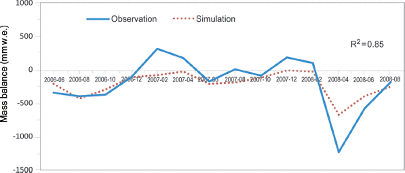
Fig. 7. Temporal variations of the simulated and observed glacier mass balance for Zhadang glacier. Date format is yyyy-mm.
7. Water Balance Analysis
Water balance was calculated using model results, glacier melt, evaporation, etc., following
where WB is the water balance (mm).
The simulated water balance in the Qugaqie and Zhadang basins shows precipitation changes between 383 and 621 mm with a large elevation gradient (Table 4). Precipitation in the Zhadang basin was 27% higher than in the whole Qugaqie basin in 2007 and 2008. The climate was relatively dry in 2006 and relatively humid in 2008. The ratio of solid rainfall fluctuated between 43% and 68%. Due to the high elevation of the Zhadang basin, the proportion of solid precipitation was >50% of annual precipitation. Land surface evaporation and snow evaporation were between 208 and 247 mm a−1 and were relatively low in Zhadang, which is covered by large glacier areas. The simulated runoff in the Qugaqie basin was in the range 705–874 mm, while the range in the Zhadang basin was 1051–1502 mm, both generally lower than observed. Glacier melt was 1084–1167 mm, indicating that glacier runoff played a crucial role in the Qugaqie basin.
Table 4. The simulated water balance in the Qugaqie and Zhadang basins
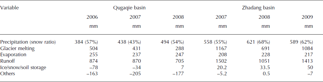
Water balance analyses in the upstream and downstream areas showed that the water storage of the whole basin was negative (Table 4). In the JAMS/J2K model, we could not explain the origin of the extra input water. However, previous studies have found that the frozen soil/ permafrost had degraded due to climate warming in the TP, creating a deeper active ground layer (Reference Cheng and WuCheng and Wu, 2007) and variations of runoff, especially during winter (Reference Liu, Xie, Gong, Wang and XieLiu and others, 2011). In the Qugaqie basin, frozen soil was widely developed (Reference TianTian and others, 2009), changing the heat and energy exchange, land surface albedo, soil heat capacity, land surface evaporation, etc., when freezing or thawing (Reference Li, Nan and ZhaoLi and others, 2002). We can suppose that as the frozen soil thaws, it will release the partially stored water that runs into the river. It is possible that some proportion of the negative water balance in the Qugaqie basin was caused by frozen soil changes. In the Zhadang basin, the water balance was almost zero or positive. This may be because the basin has a larger proportion of glacier areas and less impact on frozen soil. On the other hand, snow storage may also impact the water balance in the region. Previous studies have found that in the Nam Co basin >90% of precipitation occurred during the monsoon season (June to September) (Fig. S4 (http://www.igsoc.org/hyperlink/14j170_supp.pdf); Reference KangKang, 2011; Reference Zhang, Xie, Yao, Liang and KangZhang and others, 2012). Over the period 2005–12, the observed mass loss rate of Zhadang glacier averaged ∼1200 mm w.e. a−1 (Qu and others, 2015). The clear negative mass balance of Zhadang glacier confirms that the snowline altitude may be higher than that of the whole glacier (Reference KangKang and others, 2015). This means precipitation during the monsoon was almost entirely accounted for, by rapid melting. Compared to the large amount of precipitation during the monsoon, the runoff from stored winter snow was smaller than the summer precipitation.
8. Conclusions
The distributed hydrological model JAMS/J2K was used to simulate glacier runoff and mass balance in the Qugaqie basin and Zhadang sub-basin on the southern TP. According to the calibration and validation, RSA results indicated that the glacial parameters were the most sensitive. The runoff simulation was improved using a scheme combining the temperature, global radiation (G2) and the snow/ice refreezing process (S3). The simulated Zhadang glacier mass balance is in good agreement with observations, suggesting that the J2K model is suitable for simulating glacier mass-balance changes, especially during the melt season.
The application of the J2K model with the combined G2 and S3 algorithm (glacier and snow modules) showed that glacier meltwater accounted for >50% of the total annual streamflow in the upstream Zhadang sub-basin and the Qugaqie basin, with the largest contribution during June and July (78.94% and 81.35%, respectively). The result of the water balance in the Qugaqie basin revealed that snowmelt largely accounted for the total runoff in the upstream and downstream areas.
In the glacial basin of the TP, the sensitivity analysis and parameter optimization of hydrological models can improve the simulation results based on the glacier-/snowmelt combination method. However, the lack of a frozen soil module in the hydrological model will affect the simulation, especially under the influence of climate change. This will need further study in the future.
Acknowledgements
This study was supported by the National Natural Science Foundation of China (41121001, 41190081 and 41190083), the Global Change Research Program of China (2013CBA01801), the Chinese Academy of Sciences (KJZD-EW-G03-04) and the Academy of Finland (264307). We thank the reviewers, whose valuable comments helped to improve the manuscript, J. Schulla for his suggestions concerning the modelling, and the staff of Nam Co station for the observations.


