


1. INTRODUCTION
In the currently warming climate, meltwater runoff from glaciers and ice caps, especially in the Arctic, is a major contributor to sea-level rise (Church and others, Reference Church2011; Jacob and others, Reference Jacob, Wahr, Pfeffer and Swenson2012; Machguth and others, Reference Machguth2013; Mernild and others, Reference Mernild, Liston and Hiemstra2014; Moon and others, Reference Moon, Ahlstrøm, Goelzer, Lipscomb and Nowicki2018). It is expected that glaciers and ice caps will lead to 81 ± 43 mm of sea-level rise by 2050, assuming current acceleration (Meier and others, Reference Meier2007; Radić and Hock, Reference Radić and Hock2011; IPCC, Reference Stocker, Qin, Plattner, Tignor, Allen, Boschung, Nauels, Xia, Bex and Midgley2013). The Arctic is experiencing greater warming than the global average through feedbacks caused by changes in sea-ice extent, surface reflectivity and air temperature, a process known as the ‘Arctic amplification’ (Manabe and Stouffer, Reference Manabe and Stouffer1980; Serreze and Francis, Reference Serreze and Francis2006; Serreze and others, Reference Serreze, Barrett, Stroeve, Kindig and Holland2009).
The High Arctic archipelago Svalbard has a glacierized area of ~34 000 km2 (Nuth and others, Reference Nuth2013), equivalent to 5% of the world's land-ice mass outside of Greenland and Antarctica (Pfeffer and others, Reference Pfeffer2014; Aas and others, Reference Aas2016). Glaciers cover ~60% of the land area of Svalbard (Hagen and others, Reference Hagen, Kohler, Melvold and Winther2003) and, if melted, could potentially contribute 14–26 mm to global sea-level rise (Radić and Hock, Reference Radić and Hock2010; Huss and Farinotti, Reference Huss and Farinotti2012; Martín-Español and others, Reference Martín-Español, Navarro, Otero, Lapazaran and Błaszczyk2015). Mean annual temperature in Longyearbyen has increased by 0.25 K decade−1 over the past 100 years (Førland and others, Reference Førland, Benestad, Hanssen-Bauer, Haugen and Skaugen2011), with most of the warming in the more recent period, since 1975 (~1.0 K decade−1); the strongest recorded warming in Europe (Førland and others, Reference Førland, Benestad, Hanssen-Bauer, Haugen and Skaugen2011; Nordli and others, Reference Nordli, Przybylak, Ogilvie and Isaksen2014). The recent warming is most pronounced in winter and spring and temperatures are expected to continue to increase in the 21st century (IPCC, Reference Stocker, Qin, Plattner, Tignor, Allen, Boschung, Nauels, Xia, Bex and Midgley2013). Simultaneously, over the period 1964–97, precipitation in Longyearbyen has increased by 1.7% decade−1 (Førland and Hanssen-Bauer, Reference Førland and Hanssen-Bauer2000). In terms of glacier mass balance, however, this weak increase is not enough to compensate for effects of the warming. Svalbard glaciers show a declining mass-balance trend since 1967, when the first glaciological measurements were started (WGMS, Reference Zemp, Nussbaumer, Gärtner-Roer, Huber, Machguth, Paul and Hoelzle2017; Østby and others, Reference Østby2017).
In northwest Svalbard, the Kongsfjord basin near Ny-Ålesund plays a crucial role in scientific research in oceanography, meteorology, biology, ecology and land surface processes (hydrology, glaciology). In Kongsfjord, there are glaciers of different shapes and sizes and with different dynamic behaviour (Liestøl, Reference Liestøl1988; Hagen and others, Reference Hagen, Liestøl, Roland and Jørgensen1993). Studying mass balance of these glaciers is important for understanding the present trend of glacier retreat as well as to quantify fresh water discharge to the fjord. Apart from glacier runoff, another significant source of fresh water to the fjord in this region is meltwater from seasonal snow in the nonglacierized area. Freshwater runoff at the base of tidewater glaciers creates a buoyant plume when entering the fjord (Cowton and others, Reference Cowton, Slater, Sole, Goldberg and Nienow2015; How and others, Reference How2017) and mixes with the fjord water at different vertical depth affecting the fjord's circulation (Sundfjord and others, Reference Sundfjord2017). Plumes bring nutrients and plankton to the fjord surface, propagating their impact through the food chain to a wide range of species, and thus plays a crucial role in the fjord ecosystem (Lydersen and others, Reference Lydersen2014). Accurately quantifying the spatial and temporal distributions of meltwater runoff is, therefore, crucial for understanding the fjord system. Insight into runoff can only be gained through distributed modelling; Kongsfjord is particularly well suited for this task since long-term records (the longest in Svalbard) of glacier data exist for model calibration and validation.
Models have been widely used to simulate mass balance of glaciers from regional to global scales ranging in complexity from conceptual degree day models (Hock, Reference Hock2003; Nuth and others, Reference Nuth, Schuler, Kohler, Altena and Hagen2012) to physically-based energy-balance models (Hock, Reference Hock2005; Arnold and others, Reference Arnold, Rees, Hodson and Kohler2006). Energy-balance models consider all the energy fluxes interacting with the glacier surface to compute surface temperatures T S; the energy equivalent of T S>0 °C is used to calculate melt at the glacier surface. Meltwater percolates through the snowpack and may refreeze, depending on the subsurface temperature; any excess meltwater contributes to runoff. Refreezing plays a crucial role in the mass budget of Arctic glaciers as it increases the temperature and density of the snowpack, and reduces and delays mass loss through runoff (Wright and others, Reference Wright2007; Reijmer and others, Reference Reijmer, van den Broeke, Fettweis, Ettema and Stap2012). Furthermore, heat released by refreezing has a major impact on the thermal structure of a glacier (Poinar and others, Reference Poinar, Joughin, Lenaerts and van den Broeke2017). Refreezing below the previous year's summer surface in the firn area is known as internal accumulation (Schneider and Jansson, Reference Schneider and Jansson2004), which is not captured by conventional mass-balance monitoring. In contrast to non-polar regions, refreezing strongly affects the mass balance of High Arctic glaciers, mainly due to the strong seasonal temperature cycle (Bliss and others, Reference Bliss, Hock and Radić2014). Very cold winters with relatively little or no insolation lead to cold snowpacks, increasing the potential for refreezing of percolated meltwater during the melt season and storage of water in the snow or firn after the melt season.
Previous modelling studies of mass balance in the Kongsfjord region mainly focused on four glaciers: Austre Brøggerbreen (BRB), Midtre Lovénbreen (MLB), Kongsvegen (KNG) and Kronebreen-Holtedahlfonna (HDF) (Table 1). All of these studies have focused on either single glaciers (Bruland & Hagen, Reference Bruland and Hagen2002) or partial areas of Kongsfjord (Lefauconnier and others, Reference Lefauconnier, Hagen, Pinglot and Pourchet1994a; Kohler and others, Reference Kohler2007; Rasmussen and Kohler, Reference Rasmussen and Kohler2007; Nuth and others, Reference Nuth, Schuler, Kohler, Altena and Hagen2012; Van Pelt and Kohler, Reference Van Pelt and Kohler2015). In this study, meltwater production is simulated considering all glaciers in the Kongsfjord basin, and additionally, we simulate seasonal snow in the nonglacierized area. This enables us to distinguish runoff contributions to the fjord from glaciers and land. Glacier and seasonal snow runoff modelling over entire catchments is required to estimate the total water budget, as has been done in several glacierized catchments in the world (e.g. Himalaya, Alps, Central Asia, Alaska, Andes) (Verbunt and others, Reference Verbunt2003; Jeelani and others, Reference Jeelani, Feddema, van der Veen and Stearns2012; Duethmann and others, Reference Duethmann2015; Bring and others, Reference Bring2016; Mernild and others, Reference Mernild2016; Valentin and others, Reference Valentin, Hogue and Hay2018). The long-term simulation allows us to detect trends in seasonal snow amounts and the climatic mass balance (CMB) and its components, and relate them to transient climate conditions. We estimate and analyze the long-term CMB evolution of the entire glacierized area of Kongsfjord basin, and quantify runoff into the fjord from glaciers and from the seasonal snow of the nonglacierized area. Simulations are performed with a surface energy balance – firn model (Van Pelt and Kohler, Reference Van Pelt and Kohler2015), which has been extended with a soil model (Westermann and others, Reference Westermann, Boike, Langer, Schuler and Etzelmüller2011) to simulate seasonal snow in nonglacierized parts of the domain.
Table 1. Previous mass-balance studies on four glaciers of Kongsfjord basin

2. STUDY AREA
Kongsfjord is open to the sea to the west and is surrounded by glaciers to the south, east, and north (Fig. 1). The glaciers to the south are small land-terminating glaciers (average area per glacier ~6.5 km2), whereas the glaciers to the east and north are mainly large tidewater glaciers (>50 km2). The total nonglacierized area (tundra, hills, and nunataks) amounts to 293 km2 and accounts for 20% of the Kongsfjord basin (~1440 km2).
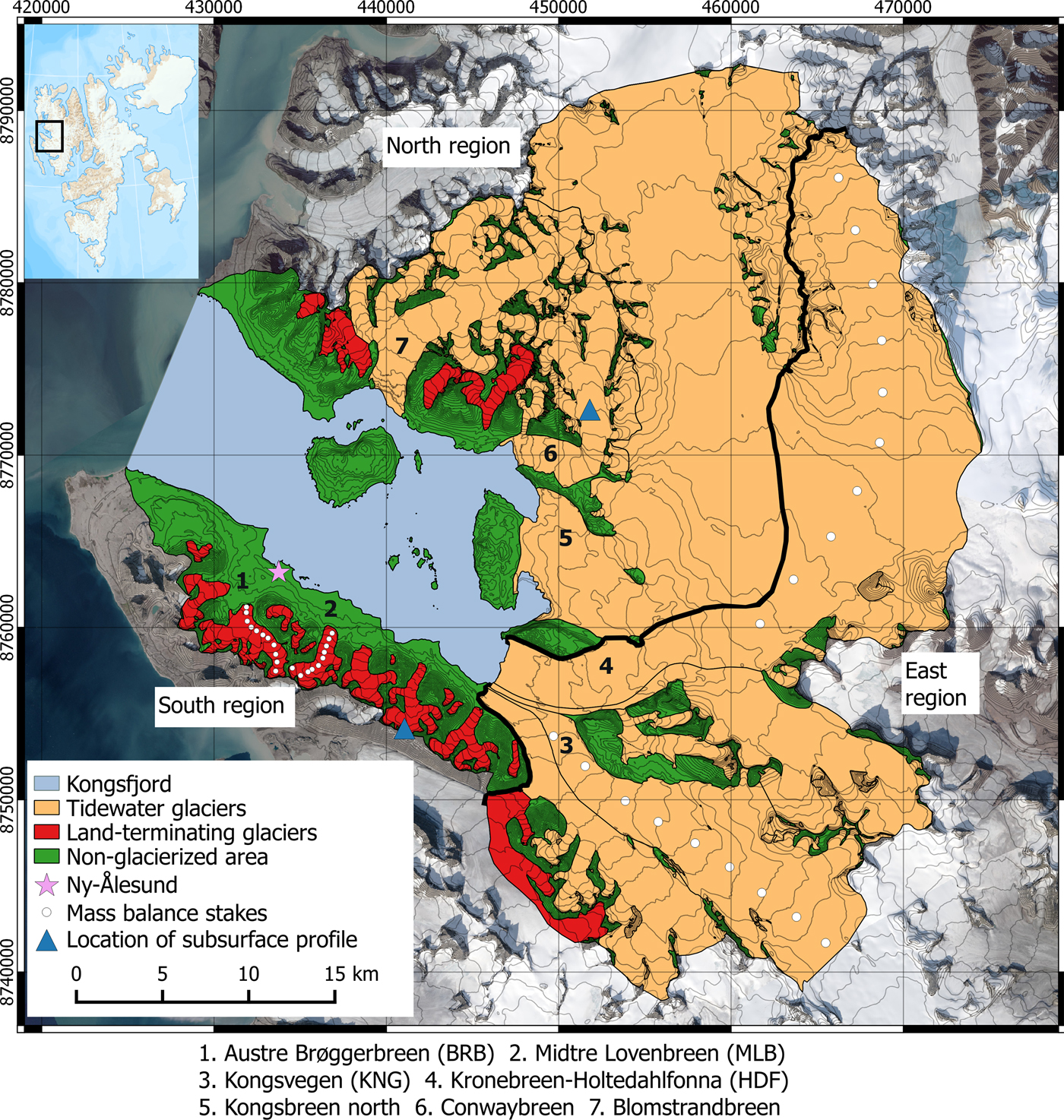
Fig. 1. Kongsfjord basin; Orange colour indicates tidewater glaciers, red colour indicates land-terminating glaciers, and green colour indicates non-glacierized area. Individual glaciers are shown with the thin black line. Thick black lines divide east region from south region and north region from east region. Mass-balance stakes of the four mass balance glaciers are shown with white dots. Ny-Ålesund is shown with magenta star. Blue triangles indicate the locations (elevation 610 m a.s.l.) where subsurface density has been investigated. The background is Landsat mosaic image.
In this study, we divide the glacierized area of Kongsfjord basin into three subregions; south (~42 km2), east (~ 573 km2) and north (~533 km2) (Figs 1, 2). Glaciers in south region are all land-terminating, low-lying and relatively slow moving (Hagen and others, Reference Hagen, Liestøl, Roland and Jørgensen1993). The east region contains two large tidewater glacier systems; Kongsvegen-Sidevegen and Kronebreen, the latter draining the ice fields of Holtedahlfonna (HDF) and Infantfonna. KNG is a surge-type glacier currently in its quiescent phase, flowing at low velocities (2–8 m a−1) and undergoing surface steepening (Hagen and others, Reference Hagen, Melvold, Eiken, Isaksson and Lefauconnier1999; Kohler and others, Reference Kohler2007; Nuth and others, Reference Nuth, Schuler, Kohler, Altena and Hagen2012). Kronebreen (KRB), which shares its terminus with KNG, is a fast-flowing tidewater glacier (300–800 m a−1; Kääb and others, Reference Kääb, Lefauconnier and Melvold2005). It has experienced two periods of rapid frontal retreat, ~ 3 km between 1966 and 1980, and ~1 km between 2011 and 2013 (Nuth and others, Reference Nuth, Schuler, Kohler, Altena and Hagen2012, Reference Nuth2013); this most recent retreat is still ongoing. The north region of the basin contains three tidewater glaciers (Blomstrandbreen, Conwaybreen and Kongsbreen, from west to east) and a few smaller land-terminating glaciers (Hagen and others, Reference Hagen, Liestøl, Roland and Jørgensen1993). The tidewater glaciers in this area vary in their dynamic behaviour and contribute substantial mass to the fjord through calving (Liestøl, Reference Liestøl1988; Lefauconnier and others, Reference Lefauconnier, Hagen and Rudant1994b). Blomstrandbreen surged in 2007 (Sund and Eiken, Reference Sund and Eiken2010; Mansell and others, Reference Mansell, Luckman and Murray2012; Burton and others, Reference Burton, Dowdeswell, Hogan and Noormets2016). Kongsbreen North was observed to move at ~2.8 m d−1 in autumn 2012 (Schellenberger and others, Reference Schellenberger, Dunse, Kääb, Kohler and Reijmer2015).
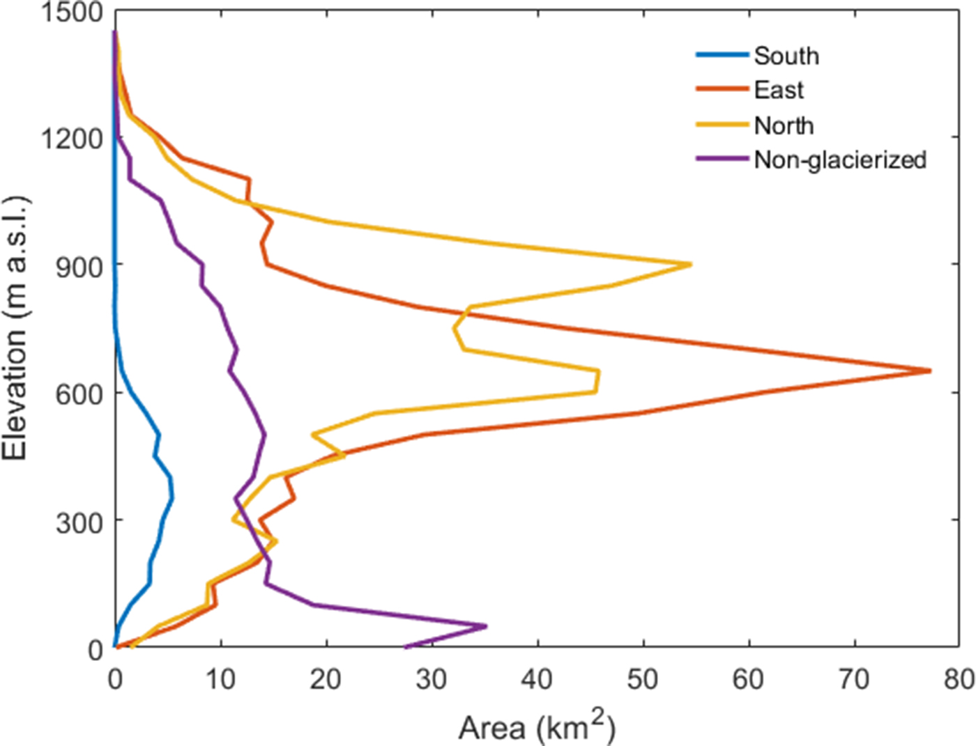
Fig. 2. Regional hypsometries of three regions. Elevation interval is 50 m. Maximum elevation is 1417 m a.s.l.
A meteorological station is situated on the southwest side of the fjord at Ny-Ålesund (78.92o N, 11.91o E). We use observational data from four glaciers (Fig. 1) (Kohler, Reference Kohler2013) monitored by the Norwegian Polar Institute (NPI) to calibrate and validate the model; two tidewater glaciers, HDF and KNG, and two land-terminating glaciers, BRB and MLB.
3. DATA
3.1. Surface DEM and glacier mask
We use a Digital Elevation Model (DEM) with a 5 m horizontal resolution, constructed by the NPI from aerial surveys in 2009 and 2010 (NPI, 2014), averaging values onto a 250 m × 250 m model grid. A recent model grid and the most recent glacier mask (König and others, Reference König, Nuth, Kohler, Moholdt and Pettersen2014) is used throughout the study period. Elevation and glacier outlines are assumed to be constant throughout the simulation period.
3.2. Meteorological input
To force the model, we use 6 hourly weather station data from Ny-Ålesund (air temperature, air pressure, cloud cover and relative humidity), and downscaled precipitation data derived from the ERA-Interim re-analysis of the European Center for Medium-Range Weather Forecast (Dee and others, Reference Dee2011). Pressure, cloudiness and humidity records from Ny-Ålesund are extrapolated to the model grid using fixed lapse rates, extracted from HIRLAM regional climate model output used in Van Pelt and Kohler (Reference Van Pelt and Kohler2015). In this work, the temperature lapse rate (TLR) is an adjustable parameter, the calibration of which is discussed in section 4.2. Precipitation from ERA-Interim is available from 1979 at 6-h intervals and at ~80 km horizontal resolution (Dee and others, Reference Dee2011). Østby and others (Reference Østby2017) downscaled this product to 1 km resolution over Svalbard using the linear theory of orographic precipitation (Smith and Barstad, Reference Smith and Barstad2004). In this study, we re-grid the 1 km product to our model domain by linear interpolation and apply a spatial linear correction derived from the measured winter mass balance, to reduce the biases of ERA-Interim precipitation.
3.3. Stake and glacier-wide mass balance
Mass-balance measurements of the two land-terminating glaciers BRB and MLB started in 1967 and 1968, respectively, while monitoring of KNG and HDF started in 1987 and 2004, respectively (WGMS, Reference Zemp, Nussbaumer, Gärtner-Roer, Huber, Machguth, Paul and Hoelzle2017). Seasonal mass balance is measured using stakes drilled into firn/ice along the glacier centrelines (Fig. 1). Stakes are measured twice a year in April and September to yield winter (b w) and summer (b s) balances. These point measurements (henceforth referred to as stake balances) are then extrapolated using the glacier hypsometry to calculate glacier-wide winter (B w), summer (B s) and net (B n) mass balances, assuming a functional relationship between mass balance and elevation. We use stake balances (winter and summer) for calibration of climate parameters of the model (section 4.2).
4. MODEL AND SET UP
4.1. Model description
The model employed in this study simulates mass and energy exchange between atmosphere, surface and the underlying snow, firn and /or ice and it has been used previously by Van Pelt and Kohler (Reference Van Pelt and Kohler2015) for the glacier system KNG and HDF. Here, we use a different precipitation product for forcing and add a separate subsurface scheme for the nonglacierized part of the domain to expand the application to the entire Kongsfjord basin.
The model iteratively solves the energy-balance equation for each time step to calculate the surface temperature. The surface temperature is capped at the melting point and excess energy is used to melt the surface. The meltwater enters the subsurface snow/firn pack and serves as input to the subsurface module.
The subsurface module is an update (Reijmer and Hock, Reference Reijmer and Hock2008) of the SOMARS model (Simulation Of glacier Mass balance And Related Subsurface processes; Greuell and Konzelmann (Reference Greuell and Konzelmann1994)), which simulates the evolution of vertical profiles of temperature, density and water content and which has been repeatedly applied on Svalbard (Van Pelt and others, Reference Van Pelt2012, Reference Van Pelt2014, Reference Van Pelt, Pohjola and Reijmer2016b; Østby and others, Reference Østby, Schuler, Hagen, Hock and Reijmer2013; Østby and others, Reference Østby2017). Briefly, percolated meltwater refreezes, depending on the subsurface temperature and density of snowpack in each layer and excess meltwater, if any, is routed vertically according to a tipping-bucket scheme. As percolated meltwater refreezes, it releases latent heat, which increases the temperature of the snowpack. Apart from gravitational densification, refrozen meltwater increases the density of the snowpack. Runoff occurs at the firn/ice transition in case a snowpack is present or at the surface in case of bare-ice exposure. The model does not consider any horizontal transport of water in between grid cells since it requires explicit treatment of surface and subsurface drainage, which is beyond the scope of the study. The subsurface model comprises a vertically adjustable grid of 100 layers, the thickness of which increases with depths by merging the 15th, 30th and 45th layers, and which vary from 0.1 m to 0.8 m. For the nonglacierized area, a subsurface soil model (Westermann and others, Reference Westermann, Boike, Langer, Schuler and Etzelmüller2011) connected with the energy-balance model simulates the heat conduction in the soil below the snowpack.
The CMB is the sum of the mass gain due to precipitation, riming at the surface and mass loss due to runoff, sublimation or evaporation. The winter balance refers to the period between 1 September of the previous year and 15 April of the current year, while summer balance corresponds to the period between 16 April and 31 August. The net balance is calculated as the sum of the winter and summer balances i.e. it covers the period between 1 September of the previous year and 31 August of the present year. Annual melt, refreezing and runoff are also calculated over the same period.
4.2. Calibration of parameters
Van Pelt and Kohler (Reference Van Pelt and Kohler2015) calibrated parameters determining incoming shortwave and longwave radiation, turbulent exchange coefficient and the albedos of snow and firn. Here, we adopt their parameter values without further refinement but calibrate TLR to achieve optimal agreement between modelled and measured stake summer balances at four glaciers (BRB, MLB, KNG and HDF; Fig. 3) by minimizing the RMSE value. Model calibration experiments are run over the observation period at selected grid points where observational data exist. Table 2 presents the calibrated parameter values used for the model application to the whole domain. We used similar TLRs for glaciers close to their respective calibrating glaciers, i.e. we use the HDF TLR for the glaciers in the north and the MLB TLR for the south side of the fjord. Time series of glacier-wide winter (B w), summer (B s) and net balance (B n) of the four mass-balance glaciers BRB, MLB, KNG and HDF (Figs 4a–d) demonstrate that the model reproduces year to year variability of mass balance very well, thus giving confidence in the interannual variability of precipitation forcing and TLR calibration.

Fig. 3. Best match of modelled and measured stake winter (b w, blue) and summer (b s, Red) balance for all four mass balance glaciers (a) Austre Brøggerbreen (BRB), (b) Midtre Lovénbreen (MLB), (c) Kongsvegen (KNG) and (d) Holtedahlfonna (HDF) after calibration.

Fig. 4. Modelled (solid line) and measured (dashed line) winter (B w), summer (B s) and net (B n) mass balances of (a) Austre Brøggerbreen (BRB), (b) Midtre Lovénbreen (MLB), (c) Kongsvegen (KNG) and (d) Holtedahlfonna (HDF) (right axis). The left-hand side of each panel shows the hypsometry of the respective glacier (left axis).
Table 2. Calibrated temperature lapse rates for mass-balance glaciers. Bias is defined as mean difference between modelled and measured mass balance

4.3. Initialization
An initialization run is performed to generate suitable subsurface conditions (temperature, density and water content) for the start of the simulation in 1979. At the start of the initialization, the density corresponds to that of ice (900 kg m−3), with a constant temperature of 270 K and zero water content. We perform 40 years of initialization in two steps, first running the model from 1979 to 1999 and then starting the second iteration from the final state of the first iteration over the same period.
5. RESULTS AND DISCUSSION
5.1. Climatic mass balance
The area-averaged climatic mass balance, snowfall, rainfall, melt, refreezing and runoff over the period 1980–2016 for the entire glacierized basin and the three subregions are shown in Table 3. Figure 5 shows spatial distributions of precipitation, melt, refreezing and climatic mass balance. Glaciers on the south and east sides of the fjord receive less snowfall compared with the glaciers in the north, while overall melt rates are highest in the south. The modelled mean CMB of glacierized area of Kongsfjord is positive (+0.23 m w.e. a−1) for the period 1980–2016. The CMB varies considerably between regions, however, with a strongly negative CMB in the south (−0.43 m w.e. a−1), a weakly negative mass balance in the east (−0.08 m w.e. a−1) and positive mass balance in the north (+0.61 m w.e. a−1). We found glacier-wide mass losses for the (land-terminating) glaciers on the south side, in agreement with the observed retreat (Rippin and others, Reference Rippin2003; Kohler and others, Reference Kohler, König, Nuth and Villaflor2018). Glaciers in the north are at higher elevations, and experience on average 56% more snowfall and 59% less melt compared with glaciers in the south region. Glaciers in the north and east are mostly tidewater glaciers and lose mass due to calving. For HDF, calving rates at its tidewater terminus KRB have previously been estimated at −0.42 ± 0.10 m w.e. a−1 for 1966–2007 (Nuth and others, Reference Nuth, Schuler, Kohler, Altena and Hagen2012), which suggests that the total mass balance is much more negative than the simulated CMB of −0.05 ± 0.26 m w.e. a−1 for 1980–2016.
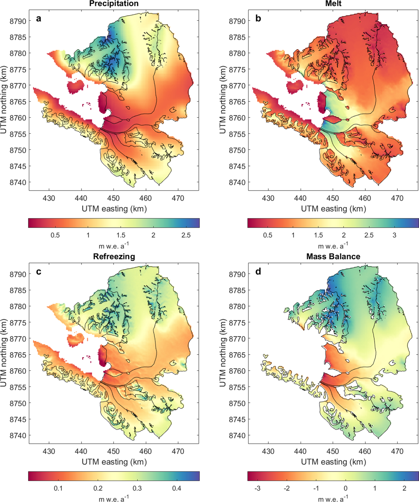
Fig. 5. Long-term spatially distributed pattern of (a) precipitation, (b) melt, (c) refreezing and (d) climatic mass balance averaged over the simulation period 1980-2016. (a–c) are for the entire Kongsfjord basin while (d) shows only the glacierized area.
Table 3. Area-averaged glacier wide climatic mass balance (B w, B s, B n), melt, refreezing and runoff for three regions and entire glacierized area, 1980–2016

Overall, refreezing comprises 17% of the total accumulation from precipitation and moisture deposition for the entire glacierized part of the basin. Average refreezing amounts to 0.24 m w.e. a−1 and consists of similar contributions of refreezing of percolating water (0.12 m w.e. a−1) in spring/summer and refreezing of stored irreducible and slush water (0.12 m w.e. a−1) in winter. For comparison, a mean value for total refreezing of 0.30 m w.e. a−1 was found on HDF and KNG by Van Pelt and Kohler (Reference Van Pelt and Kohler2015). Refreezing varies spatially, with lower values in the south (0.21 m w.e. a−1) than the north region (0.27 m w.e. a−1). The higher refreezing rates in the north region are most likely due to the relatively larger accumulation zones that allow deeper water storage in firn and refreezing in the winter season. Substantial refreezing also occurs in seasonal snow on soil (0.21 m w.e. a−1), most of which is related to rainfall events during the cold season. Major refreezing events after heavy rainfall during the core winter season can cause the formation of basal ice in the snowpack (Hansen and others, Reference Hansen2014; Van Pelt and others, Reference Van Pelt2016a, Reference Van Pelt, Pohjola and Reijmer2016b), which can dramatically impact food supplies of grazing herbivores in Svalbard (Kohler and Aanes, Reference Kohler and Aanes2004).
Time series of annual climatic mass balance, snowfall, rain, melt and refreezing are shown in Fig. 6 for the entire glacierized area and for the three subregions. The area-averaged net balance has a weakly negative but nonsignificant trend for the entire glacierized basin and the south and north regions over the simulation period, whereas the trend is significant for the east region (Table 4). Summer balance has a weakly negative but significant trend for the entire glacierized area, east and north region, while the trend in the south region is nonsignificant over the simulation period 1980–2016 (Table 4).
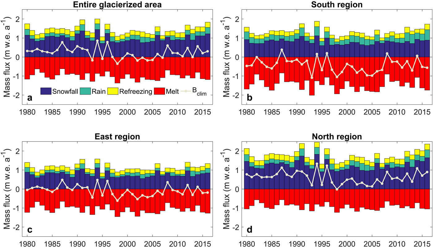
Fig. 6. Glacier area-averaged climatic mass balance and its components over the simulation period 1980–2016 for the (a) entire glacierized area, (b) south region, (c) east region and (d) north region. The climatic mass balance of a year is calculated between 1 September of the previous year and 31 August of the present year.
Table 4. Climatic mass-balance trend of three subregions and entire glacierized area with their corresponding p values

We find an increasing trend of 0.12 K a−1, 0.04 K a−1 and 0.09 K a−1 (with p < 0.005 for all) for mean winter, summer and annual temperatures respectively (Fig. 7) over the simulation period 1980–2016. We find correlations of −0.32 (p < 0.06) and 0.77 (p < 0.01) between net mass balance and mean summer temperature, and between net mass balance and annual snowfall, respectively, for the entire glacierized area. Net mass balance has a significant correlation to the annual snowfall for the south, east and north regions, with the strongest correlation observed in the latter region (Table 5). The anticorrelation of net mass balance with mean summer temperature is weakest and nonsignificant for north region, however, the anticorrelation is stronger in the east and south regions (Table 5), which indicates that mass balance of glaciers in the south and east is more sensitive to temperature than in the north. Winter precipitation shows a positive but nonsignificant trend for the entire glacierized basin (+0.0023 m w.e. a−2, p < 0.4) as well as the south (+0.0024 m w.e. a−2, p < 0.3), east (+8.9 × 10⁻⁴ m w.e. a−2, p < 0.7) and north (+0.0038 m w.e. a−2, p < 0.3) regions over the simulation period 1980–2016. There is a significant increasing trend in summer temperature, which induces a negative and significant trend in summer balance for the entire glacierized basin as well as in two of the subregions (east and north). However, the summer balance is compensated to a certain extent by the slightly increasing winter precipitation for the entire glacierized area as well as all subregions, thereby yielding a nonsignificant trend in the net climatic mass balance.
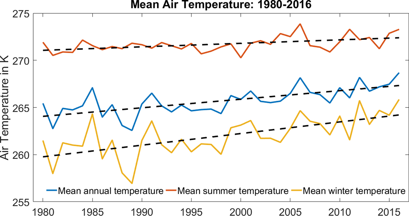
Fig. 7. Temperature (winter, summer and annual) for the period 1980–2016. Mean winter temperature increased around 2 K between 1980 and 2016. The trends for winter, summer and annual temperature are 0.12 K a−1, 0.03 K a−1 and 0.09 K a−1, respectively, shown with black dashed line.
Table 5. Correlation between winter snowfall and CMB and temperature and CMB for three subregions and entire glacierized area

5.2. Runoff
Figure 8 shows time series of total annual runoff from the glacierized subregions and nonglacierized areas. Runoff from the nonglacierized area is mainly due to snowmelt and comprises ~16% of the total runoff from the whole basin over the simulation period. Runoff from seasonal snow is limited by the amount of cumulative snowfall in the cold season. Area-averaged runoff from glaciers is largest in the south, followed by the east and north regions (Table 3). Nevertheless, total glacier runoff is smallest in the south due to the small glacier area; the east region contributes the most fresh water to the fjord (Fig. 8). Differences in runoff between glacierized and nonglacierized areas are largest in years with warm summers due to high rates of glacier ice melt after the disappearance of the seasonal snow.
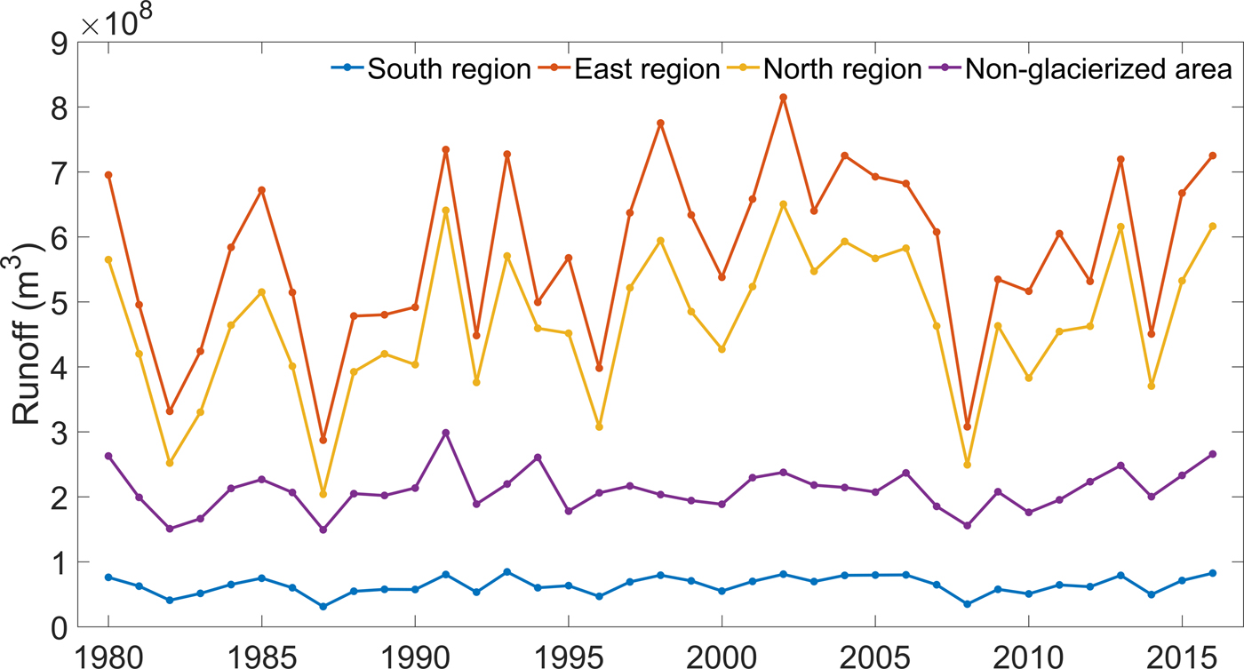
Fig. 8. Total annual runoff from the glacierized and non-glacierized areas over the simulation period 1980–2016. Total runoff from non-glacierized area contributes 16% of the total freshwater to the fjord. Runoff from seasonal snow is limited by the winter snowfall whereas runoff from the glacierized area is from both snow and ice melt from glaciers.
We find an increasing and statistically significant trend in annual runoff from the glacierized area (6.83 × 10⁶ m3 a−1 with p < 0.09), and the east (3.47 × 10⁶ m3 a−1 with p < 0.1) and north (3.1 × 10⁶ m3 a−1 with p < 0.08) regions over the simulation period, while a positive but nonsignificant trend is observed in runoff from the south region (2.51 × 10⁵ m3 a−1, p < 0.24). With future warming, runoff from all the glaciers will increase substantially (see section 5.5). Increased runoff volume will potentially lead to more rapid vertical mixing of fresh water at the tidewater glacier front, which would impact the fjord circulation (Sundfjord and others, Reference Sundfjord2017) and promote more foraging of marine mammals (Lydersen and others, Reference Lydersen2014). Increased runoff from land-terminating glaciers would lead to greater stratification and affect the physical and chemical environment of the fjord (Nowak and Hodson, Reference Nowak and Hodson2013, Reference Nowak and Hodson2015).
5.3. Decadal changes
Figure 9 shows averages of climatic mass balance, snowfall and rainfall as a function of elevation for the glacierized area of Kongsfjord basin during four periods; 1980–89, 1990–99, 2000–09 and 2010–16 (7 years). The overall positive mass-balance gradient is especially pronounced for the period 2010–16 (Fig. 9a), mainly driven by an increase in snowfall at high elevations (Fig. 9b). On average, mass balance is positive above 600 m a.s.l., with the major contribution coming from glaciers on the north and northeast side of the fjord. We find substantial increases in precipitation (both snowfall and rainfall) at higher elevations of the basin in the most recent period. However, there is no significant change in snowfall at lower elevations, although rainfall has increased substantially at all elevations. Average rainfall during the last three decades was 0.15 m w.e. a−1 and has increased by 27% in 2010–16 compared with 1980–2009. In a warmer and wetter future Svalbard climate (Førland and others, Reference Førland, Benestad, Hanssen-Bauer, Haugen and Skaugen2011), rainfall is likely to further increase; with most pronounced warming in winter, more rainfall is likely to occur also during the cold season (Van Pelt and others, Reference Van Pelt2016a).
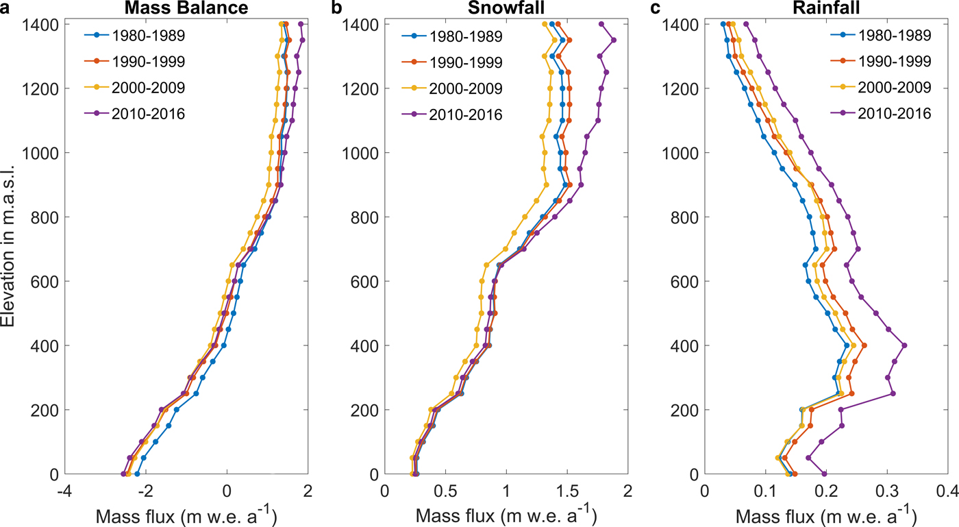
Fig. 9. Evolution of (a) climatic mass balance, (b) snowfall and (c) rainfall for four different periods as a function of elevations. CMB, snowfall and rainfall are averaged over the periods and spatially integrated within 50 m elevation bins for the glacierized area of the whole Kongsfjord basin.
The mass balance of the entire glacierized area of Kongsfjord has decreased over the last three periods (1990–99, 2000–09, 2010–16) compared with the 1980–89 period, with 2000–09 having the lowest mass balance ( + 0.08 m w.e. a−1) (Fig. 6). Melt and runoff in the 1990–99 and 2000–09 periods increased substantially compared with the 1980–89 period and decreased in 2010–16. However, melt and runoff in 2010–16 has increased by 12 and 17%, respectively compared with 1980–89 (Fig. 6). The average Equilibrium Line Altitude (ELA) of the glacierized area has increased from 437 ± 75 m a.s.l. in 1980–89 to 509 ± 153 m a.s.l. and 572 ± 110 m a.s.l. in 1990–99 and 2000–09, respectively, decreasing to 517 ± 74 m a.s.l. in 2010–16.
5.4. Subsurface variables
Figures 10a, b show the time-depth evolution of subsurface density for the period 1990–2015 at two sites; one on a glacier in the south region and the other on a glacier in the north region (locations are shown in Fig. 1). The elevation of both sites is ~610 m a.s.l., within the accumulation zone of the respective glaciers. In spite of being at similar elevations, we find significant differences in the firn density evolution at these locations. The glacier in the south region has a small accumulation area, and the proximity of the ELA inhibits the formation of a thick firn layer. Firn almost disappears at this location over the period 1998–2006, due to low snowfall and high melting. At a similar elevation in the glacier in the north region, the significantly thicker firn started depleting between 1998 and 2006, caused by low snowfall in this period, when all glaciers show most negative mass balance. The site in the north region is higher above its local ELA than the site in the south, thus leading to the formation of a thicker snow and firn pack. Due to higher snowfall in the post-2006 period, firn thickness starts to increase, especially after 2011, at both locations.
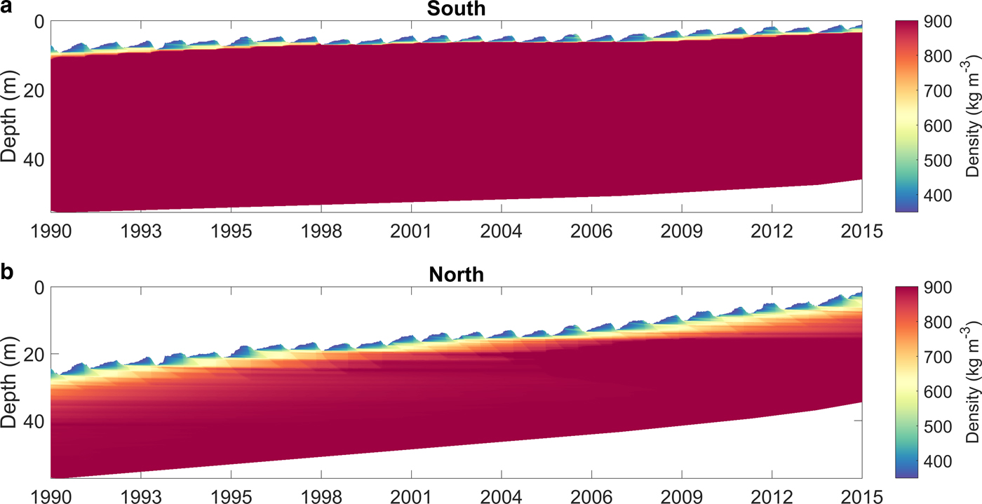
Fig. 10. Time series of simulated subsurface density at a location in the accumulation area of (a) a glacier in the south region and (b) a glacier in the north region. Locations are shown in Fig. 1; both are at an elevation of 610 m a.s.l.
5.5. Climate sensitivity
To reduce computational cost, sensitivity tests were conducted at the mass-balance stake locations of the four NPI study glaciers over the period 1979–2016. We performed multiple runs perturbing air temperature (T), precipitation (P) and cloud cover (C) uniformly over the simulation period, without considering any seasonal variability. Table 6 provides the sensitivities of net mass balance, refreezing and runoff to perturbations in T, P and C in terms of anomalies to the long-term mean of the unperturbed state for three glaciers (MLB, KNG and HDF). Altitudinal profiles of sensitivities of mass balance, refreezing and runoff for six changing climate scenarios for KNG are shown in Figure 11. Mass balance and runoff are generally more sensitive to temperature than precipitation; runoff in the accumulation zone is nearly insensitive to precipitation changes. Refreezing has a complex response to changes in precipitation and temperature (Fig. 11b). Increases in precipitation lead to increased refreezing as a thicker snowpack has a higher cold content and a larger pore volume. This promotes both refreezing of meltwater in the early melt season and refreezing of stored irreducible water after the melt season. Similarly, reduced temperatures will increase snow depth and the extent of the accumulation zone and will simultaneously enhance winter cooling, all of which contribute to enhance refreezing. With the upward migration of the ELA in a warming climate refreezing rates drop and runoff amplifies. This explains the strong nonlinearity in the mass balance and runoff sensitivity to temperature change at sites just above the present ELA (Fig. 11). Table 6 shows that an increase in cloud cover increases runoff and decreases refreezing substantially.
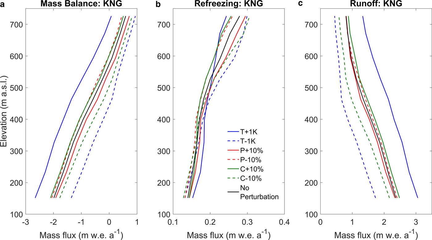
Fig. 11. Sensitivities to perturbations in temperature (T), precipitation (P) and cloud cover (C) of (a) mass balance, (b) refreezing and (c) runoff along the centreline of Kongsvegen (KNG).
Table 6. Overview of mass-balance sensitivity (δB), refreezing sensitivity (δRE) and runoff sensitivity (δRU) to changing temperature (T), precipitation (P) and cloud cover (C) of three glaciers along their central line. Units are in m w.e. a−1.

Sensitivity values of BRB are similar to MLB and therefore not shown here.
5.6. Uncertainties
A substantial source of uncertainty in the presented results comes from the small-scale variability of spatial snow distribution that is not accounted for by the orographic precipitation model. Local topography, wind speed and direction influence snow deposition and distribution in mountainous terrain like Kongsfjord basin (Hodgkins and others, Reference Hodgkins, Cooper, Wadham and Tranter2005; Lehning and others, Reference Lehning, Löwe, Ryser and Raderschall2008; Dadic and others, Reference Dadic, Mott, Lehning and Burlando2010). Ignoring the small-scale variability of accumulation leads to biases in the area-averaged mass balance as the mass balance has a nonlinear response to snow accumulation (Van Pelt and others, Reference Van Pelt2014). Another source of uncertainty is that we used a fixed topography and ice extent throughout the entire simulation, which adds uncertainty to the extrapolation of elevation-dependent meteorological parameters, such as temperature and precipitation, and to runoff due to glacier length fluctuations. A 250 m × 250 m DEM would not properly resolve the topography around smaller glaciers leading to inappropriate shading, which would lead to uncertainty in radiation budget for those glaciers.
We used fixed start and end dates to calculate the mass balance of each year. Although in a warming climate the mass-balance year may need to be redefined eventually, it is convenient for comparison and to detect trends to have fixed dates define the mass-balance year.
Extrapolation of stake data to a glacier-wide grid also leads to uncertainty. In particular, the extrapolation of winter balance may contain significant uncertainty due to potential snow accumulation variability in our study region.
We used a fixed time-invariant TLR for different glaciers over the simulation period which is another source of uncertainty in the model, as cloud condition substantially affects the TLR (Petersen and others, Reference Petersen, Pellicciotti, Juszak, Carenzo and Brock2013; Matuszko and Węglarczyk, Reference Matuszko and Węglarczyk2014; Van Tricht and others, Reference Van Tricht2016).
Finally, observations used for model calibration and validation do not include any glaciers in the north region, which increases the uncertainty of the results in this region. More observational data from this region will help to constrain uncertainties.
6. CONCLUSIONS
We use a surface energy-balance model coupled with a subsurface snow/firn model (Van Pelt and others, Reference Van Pelt2012) to simulate the long-term (1980–2016) evolution of the CMB of glaciers and the associated fresh water flux into the Kongsfjord basin. The model is forced with downscaled ERA-Interim precipitation and climate data extrapolated from the nearby meteorological station in Ny-Ålesund, on a 250 m × 250 m grid. Calibration is performed by adjusting the TLR to match the measured summer balance data.
Results indicate that glaciers of Kongsfjord basin show wide variability in mass balance from south to north and from west to east. The CMB of the entire Kongsfjord basin is estimated to an average of + 0.23 m w.e. a−1 over the simulation period. Glaciers in the north region of Kongsfjord show overall positive CMB and are least sensitive to temperature perturbations, whereas glaciers in the south and east regions show overall negative CMB and are more sensitive. The net CMB of the entire glacierized basin shows a weakly negative but nonsignificant trend, although summer balance has a negative and significant trend over the simulation period 1980–2016.
Comparison of mass-balance components during the periods 1980–89, 1990–99, 2000–09 and 2010–16 shows a lowest CMB (+0.08 m w.e. a−1) in the 2000–09 period. The most recent period (2010–16) had above-average precipitation, which could be related to recent retreat of Arctic sea-ice cover and increasing winter temperatures. Increase in snowfall is observed only at higher elevation but rainfall increases throughout the domain.
Refreezing accounts for 17% of the total mass gain and is higher in the north (0.27 m w.e. a−1) than in the south (0.21 m w.e. a−1). Snowmelt from nonglacierized areas in early summer contributes 16% of the total runoff to the fjord, while the remaining 84% is from glacier runoff. The largest contribution to total runoff comes from the east region. We find a significant increase in runoff trend over the simulation period from the entire glacierized area.
ACKNOWLEDGEMENTS
The first author received Ph.D. studentship support from ESSO-National Centre for Antarctic and Ocean Research (NCAOR), financed by the Ministry of Earth Sciences, Government of India; Grant/Award number: MoES/16/22/12-RDEAS (PhD fellowship-NPI). Additional funding came from the Polish-Norwegian Research Programme GLAERE, the Norwegian Research Council project TIGRIF, and the Norwegian Polar Institute's TW-ICE project. We thank the editor, H. Jiskoot and one anonymous referee for their insightful comments that helped to improve the manuscript. This article is NCAOR contribution no. 46/2018.


 Open access