


1. INTRODUCTION
The ablation of ice and snow at glaciers and ice sheets is of much importance for the mass balance of glaciers, and contributes both to the direct loss of mass and indirectly through the lubricating effect that meltwater can have on glacier dynamics. Despite this importance, there currently exist only two general methods of estimating ablation, using either a full energy-balance model (e.g. Kraus, Reference Kraus1973) or the positive degree day (PDD) model (e.g. Braithwaite, Reference Braithwaite1995). In energy-balance models, information about cloud cover and vertical profiles of wind speed, humidity, and air temperature are typically needed to calculate the relevant energy fluxes. However, these quantities are rarely measured in enough detail (if at all) to be able to use measured quantities. Instead, atmospheric models are often used (e.g. Sanz Rodrigo and others, Reference Sanz Rodrigo, Buchlin, van Beeck, Lenaerts and van den Broeke2013) to estimate the quantities needed, leading to significant uncertainties in the appropriate parameters. The PDD model (also known as a temperature-index model) represents the opposite extreme in that the PDD model estimates ablation using only measurements of surface air temperature and empirically calibrated degree-day factors that are usually used to scale the (above zero) temperatures to (above zero) ablation rates (with no ablation at temperatures below 0°C).
Due to the simplicity and computational efficiency of the PDD method, as well as the wider availability of surface air temperature measurements or estimates, the PDD method has been a popular alternative to the energy-balance model. In some cases, energy-balance methods simply cannot be applied, for example for historical datasets where atmospheric models are grossly inaccurate, but PDD models can still provide useful estimates of ablation (e.g. Janssens and Huybrechts, Reference Janssens and Huybrechts2000; Ohmura, Reference Ohmura2001; Wake and others, Reference Wake2009; Irvine-Fynn and others, Reference Irvine-Fynn2014; Wilton and others, Reference Wilton2017). Unfortunately, while PDD estimates of ablation have been shown to be reasonably accurate, they lack a clear physical basis and do not obviously satisfy energy conservation laws that are expected to hold. Specifically, PDD models either assume that above 0°C temperatures can immediately cause ablation regardless of how cold the ice was immediately prior to that or how long those cold temperatures lasted, or that there is a nonphysical non-0°C melt threshold (e.g. van den Broeke and others, Reference Van den Broeke, Bus, Ettema and Smeets2010). This clear inconsistency with physical expectation is one of the primary motivations of this work. While there may be other physical limitations to the PDD model (e.g. Hock, Reference Hock2003; Pellicciotti and others, Reference Pellicciotti2005; Sicart and others, Reference Sicart, Hock and Six2008), we concentrate on how to make predictions that are consistent with energy conservation while still only relying on limited measurements (temperature) as inputs.
In Section 2, we present a simplified 1-D energy balance that accounts for ice temperature and find that this physics results in a model for predicting ablation rates that is similar to the PDD model but has a physical basis. Like the PDD model, our simple model does not explicitly account for radiative energy fluxes but instead assumes that air temperature is measured and that the temperature indirectly accounts for radiation. In Section 3, we show predictions of the new model for idealized scenarios as well as for applications to Greenland where we find the model improves upon PDD estimates of ablation.
2. MODEL
2.1. New ablation model
The simplified physical model that we propose here is one in which the 1-D local temperature profile is used to calculate the vertical flux of heat, which can either go towards melting ice and hence producing ablation (thinning of ice) or can go towards warming up cold ice or cooling down warm ice (e.g. Aschwanden and others, Reference Aschwanden, Bueler, Khroulev and Blatter2012). As such, although the model is simplified significantly from a full energy-balance model (e.g. Kraus, Reference Kraus1973), it still satisfies the basic laws of physics which are expected to govern the melting of ice. Perhaps most significantly, unlike the PDD model, which assumes ice melts as soon as air temperatures are above 0°C (or has a nonphysical melt threshold), this model accounts for a delay in melting related to the warming of ice from significantly below 0°C to the melting point. This part of the heat budget is sometimes called the ‘cold content’ (Kattelmann and Daqing, Reference Kattelmann and Daqing1992; Marks and others, Reference Marks, Domingo, Susong, Link and Garen1999) in energy-balance models.
As in the classical PDD model, we assume that there exists a single measurement of surface air temperature, T a(t), made continuously in time, t and that this measurement is made at a height z = h above the surface of the glacier or ice sheet (z = 0 being defined as the glacier surface) as shown in Figure 1. We also assume that heat (potentially in the form of liquid water) can potentially percolate downwards such that there is a zone of thickness H p at the surface of the glacier that is of uniform temperature and through which heat is assumed to equilibrate (see Fig. 1). In the absence of such percolation-assisted heat transfer, heat is not expected to diffuse more than 5 m over the course of a full year (e.g. Turcotte and Schubert, Reference Turcotte and Schubert2002), but it is expected that most glaciers have a more efficient exchange of heat between the surface and some percolation depth H p. While H p may potentially vary temporally, for example due to liquid water percolation transferring heat more efficiently than thermal conduction alone, in this model we assume H p is a fixed constant for a given region. It is also assumed that this heat transfer can be accomplished with an infinitesimal amount of melt (see Section 3.2 for further discussion). H p is expected to be larger when ice is porous or fractured, allowing efficient transfer of heat downwards through either air flow or melt. The modeled temperature of this percolation region is denoted T p(t). Below this depth, it is expected that the temperature of the glacier quickly reaches its long-term average temperature since diffusion of temperature is inefficient over longer length scales (Turcotte and Schubert, Reference Turcotte and Schubert2002).
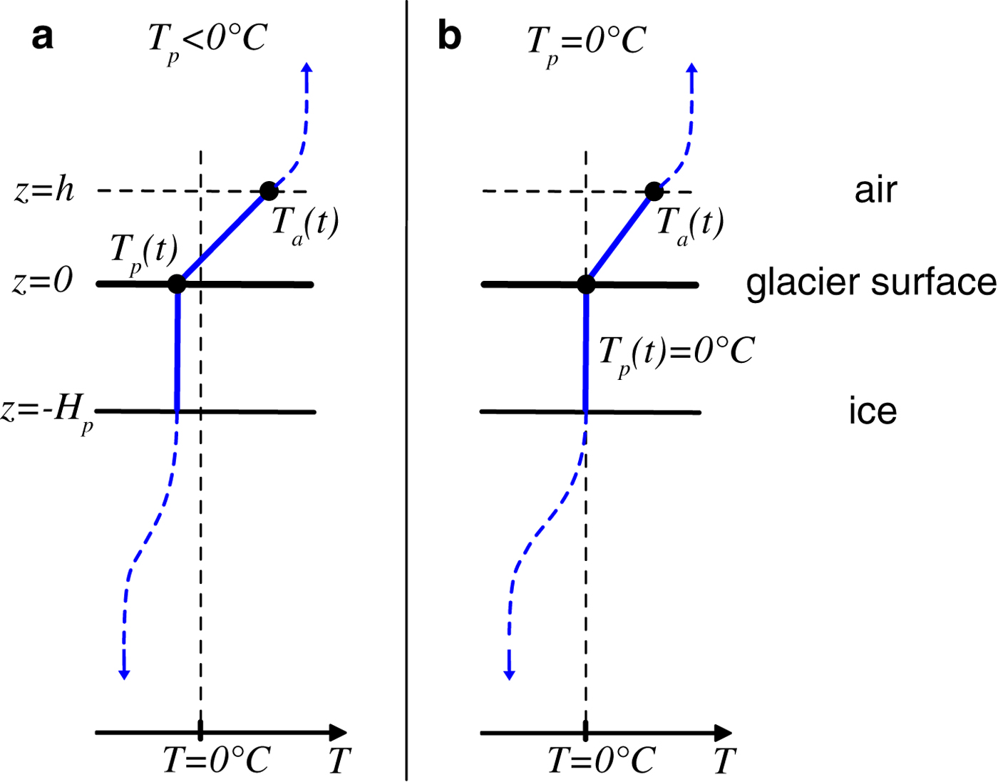
Fig. 1. Schematic of the temperature profile assumed. T a(t) is the air temperature observed at z = h. T p(t) is the modeled temperature in a ‘percolation’ zone of thickness H p. (a) A typical temperature profile when T p is <0 °C. (b) A typical temperature profile when T p is at the melting point.
In order to calculate heat fluxes, it is further assumed that the gradient of air temperature is constant from z = 0 to z = h and that there is a single effective thermal conductivity k of air. In other words, we assume there is a linear temperature profile with heat flux q given by
 $$q(t) = - k\displaystyle{{\partial T} \over {\partial z}} = - k\displaystyle{{T_a(t) - T_p(t)} \over h},$$
where this expression for heat flux assumes that radiation is important for determining T a(t) but plays no other role in the surface heat flux. In principle, k should be a material constant that is known but, in reality, it is affected by the efficiency of small-scale air turbulence and we discuss later how values of k are chosen and how they may vary spatially and temporally (see Section 2.2). The only other parameters that enter our model are the material constants ρ, c P and L, which are the density of ice, specific heat of ice and the latent heat of ice, respectively.
With the assumptions above of a simplified 1-D heat budget, conservation of energy between the percolation layer and the air implies the following governing equations for the percolation layer temperature T p(t) and ablation rate a = −dz s/dt where z s is the surface location
 $$\rho c_PH_p\displaystyle{{{\rm d}T_p} \over {{\rm d}t}} = \displaystyle{k \over h}\left( {T_a - T_p} \right),{\rm if} \, T_p \lt 0 \,\,\,{\rm or} \,\,T_a \lt 0$$
 $$T_p = 0,\quad {\rm if} \quad {\rm} T_p = 0\,{\rm and}\,T_a \gt 0$$
for T p(t) and
 $$ - \displaystyle{{{\rm d}z_s} \over {{\rm d}t}} = 0,\quad {\rm if}\,T_p \lt 0\,{\rm or}\,T_a \lt 0$$
 $$ - \rho L\displaystyle{{{\rm d}z_s} \over {{\rm d}t}} = \displaystyle{k \over h}\left( {T_a - T_p} \right),\quad {\rm if}\,T_p = 0\,{\rm and}\,T_a \gt 0$$
for a = −dz s/dt. Eqn (2a) describes the warming of the percolation layer when it is below freezing (i.e. warming of the ‘cold content’) (see Fig. 1a), whereas Eqn (3b) describes the ablation that is expected once the percolation temperature is at 0°C (see Fig. 1b), similar to how more general enthalpy methods are constructed (Aschwanden and others, Reference Aschwanden, Bueler, Khroulev and Blatter2012). In fact, H p can be thought of simply as a parameter that determines how much enthalpy is needed to account for warming the near surface of the glacier. Note that Eqn (2a) also describes the cooling of the percolation layer when T a<Tp. Ablation as described by Eqn (3) is always positive and leads only to the lowering of the surface z s; the surface z s may be expected to stay in steady state over the long term (many seasons) due to advection of ice from upstream, but this is not directly relevant to the calculation of ablation and will not be discussed further. More importantly, Eqns (2) and (3) also assume that there is negligible heat transfer from greater depths within the ice. There are two potential reasons why this might be reasonable: First, if the percolation layer thickness H p is much larger than the total annual integrated ablation ( $ \int a(t){\rm d}t$ over 1 year), then the additional heat flux caused by neglecting the lowering of the surface would be justifiably small (i.e. no additional contribution to Eqn (3)). A second reason that this heat flux could be ignored is if the long-term average temperature at depth is similar to the time-averaged percolation layer temperature. In this case, the net effect of heat transfer from depth would also be negligible (i.e. no additional contribution to Eqn (2)). In this model, we ignore these terms of the heat budget. While such terms could potentially be included, they would lead to additional parameters (like the long-term average temperature at depth) that may not be well constrained and we prefer to maintain the simpler physical model here. Accounting for these additional terms could be an avenue of future work.
Rearranging Eqns (2) and (3) yields the following two equations that can be used to directly calculate T p(t) and a(t) = −dz s/dt
 $$\displaystyle{{{\rm d}T_p} \over {{\rm d}t}} = \displaystyle{k \over {h\rho c_PH_p}}\left( {T_a - T_p} \right),\quad{\rm if}\quad T_p \lt 0\,{\rm or}\,T_a \lt 0$$
and
 $$a(t) = - \displaystyle{{{\rm d}z_s} \over {{\rm d}t}} = \displaystyle{k \over {h\rho L}}\left( {T_a - T_p} \right),\quad {\rm if} \quad T_p = 0\,{\rm and}\,T_a \gt 0$$
where Eqn (4) is an ordinary differential equation (ODE) for the percolation layer temperature T p(t) and once T p(t) is determined through Eqn (4), then Eqn (5) is an algebraic equation for the ablation rate a(t). Constants k, h, ρ, c P, H p and L are all assumed to be known. Given an air temperature time series T a(t), Eqn (5) leads to a new estimate of the ablation rate a(t). Code implementing the model is provided as a supplementary file.
2.2. Comparison with the PDD model
The model proposed in Section 2.1 has many similarities to the PDD model. Perhaps most importantly, the only time-varying quantity that needs to be measured to calculate ablation is a single local air temperature T a(t), unlike some previously suggested improvements to the PDD model (e.g. Williams and Tarboton, Reference Williams and Tarboton1999; Hock, Reference Hock2003; Pellicciotti and others, Reference Pellicciotti2005; Irvine-Fynn and others, Reference Irvine-Fynn2014). The model requires a numerical solution to an ODE, rather than having an algebraic solution like the PDD model, but this is easily accomplished with a wide range of standard numerical software with little computational effort. (Running the model for 40 years at 12-h resolution takes 6 s on a modern laptop computer; see Section 3.3.) The new model also requires an estimate of the percolation layer thickness, H p, which in some cases may not be easily measurable, though in principle it is straightforward to measure H p as the depth to which temperatures are approximately constant during the melt season. Alternatively, reasonable lower and upper bounds might also be estimated from observations of surface porosity and fracture density, which are typically available for a given field site. A brief discussion of how much H p varies spatially across Greenland is provided in Section 3.3, though a more complete spatiotemporal analysis would be useful but is beyond the scope of this work.
The current model also has the interesting feature that it mathematically simplifies to exactly the PDD model in the limit as H p → 0. Taking this limit of Eqn (4), one can determine that any air temperature T a above 0°C will immediately bring the percolation layer temperature to 0°C, and ablation will therefore occur at the rate a(t) = (k/hρL) · T a(t) given by Eqn (5), i.e. ablation is proportional to air temperature for air temperatures above 0°C, just as in the PDD model. The factor β = k/hρL can then be identified as the standard degree-day factor linking observed temperatures to ablation rate. Observations (Hock, Reference Hock2003) suggest that the degree-day factor is typically in the range 4–20 mm d−1 °C−1. With standard values of ρ = 920 kg m−3 and L = 334 kJ kg−1, this implies that k/h is in the range 14–71 W m−2 °C−1. Using h = 1 m, that would imply that the effective thermal conductivity k is in the range 14–71 W m−1 °C−1. Note that this is ~1000 times larger than the laboratory measured thermal conductivity of air, k a ≈ 0.024 W m−1 °C−1, and most of this discrepancy is due to the small-scale turbulent motions of air near the ground-surface that causes more efficient heat transfer than conduction alone. Differences in measured degree-day factors are thus expected to primarily be due to differences in this turbulence, rather than directly due to albedo or radiation as suggested by Hock (Reference Hock2003) for the PDD model, and this in turn suggests that uncertainties in k and H p may be responsible for most uncertainties in both the PDD model and the current one (including differences between snow and ice ablation rates). (For example, pockets of stagnant air in snow can decrease local turbulence and thus decrease efficiency of heat transfer and cause generally lower degree-day factors for snow. Since snow has lower albedo, this stagnation of air should correlate with albedo and thus may explain why observed degree-day factors anticorrelate with albedo as in Arendt and Sharp (Reference Arendt, Sharp, Tranter, Armstrong, Brun, Jones, Sharp and Williams1999).) This limiting behavior approaching the PDD model is most appropriate for temperate glaciers, where the temperature of glacial ice is at 0°C throughout. The present model therefore provides a physical justification for the PDD model, when applied to temperate glaciers that do not have significant ice below freezing for any portion of the year. The model also predicts that the PDD model should have a constant ablation factor (α) that is approximately zero, which is also confirmed by observations (Braithwaite, Reference Braithwaite1995). While other justification has been previously provided for the PDD model that relies on more complex energy-balance models (e.g. Ohmura, Reference Ohmura2001), the present model is novel and complementary to previous justification and expresses perhaps the simplest possible and most straightforward justification, while also clearly identifying some of the limitations of the PDD model. Importantly, the model therefore provides a physical interpretation for degree-day factors and their uncertainties as well as providing guidance for how parameters of the model might be determined when empirical calibration is not possible. While radiation has been explicitly ignored in this analysis, surface air temperature T a(t) strongly depends on radiation such that the above conclusions are not in contradiction with the observation that longwave radiation often dominates the surface energy balance (Ohmura, Reference Ohmura2001). If radiation plays an additional role beyond determining the surface air temperature, that would suggest additional complexity beyond what is described by the present model (e.g. Sicart and others, Reference Sicart, Hock and Six2008) and would also imply further limitations of the PDD model and the interpretation of degree-day factors in these scenarios.
Finally, we note that our new model predicts the opposite offset of ablation at 0°C as compared with the full PDD model as empirically calibrated by Braithwaite. In the current model, ablation is always zero at 0°C and can be zero at above 0°C, whereas the full linear PDD model as calibrated by Braithwaite has small but nonzero ablation predicted at 0°C and is always nonzero at above 0°C. One reason for the nonzero ablation at 0°C in the full PDD model is the possible bias from using daily averaged temperatures that may include part of a day that is above 0°C (Braithwaite, Reference Braithwaite1995; Hock, Reference Hock2003; van den Broeke and others, Reference Van den Broeke, Bus, Ettema and Smeets2010). We would expect that if air temperature were continuously monitored (e.g. every minute), this bias would disappear. We ignore this effect and assume that continuous temperature measurements are available and that any discretization of this, including daily averaging, will result in some small bias of the results.
3. RESULTS
3.1. General behavior of the model
Before applying the model to a real dataset, we present results for a test scenario in which the air temperature time series is idealized as the sum of two sinusoids as
 $$T_a(t) = 5^ \circ {\rm C} \cdot \left[ { - \cos \displaystyle{{2\pi t} \over {5\,\; {\rm months}}} + \sin \displaystyle{{2\pi t} \over {1\; \,{\rm month}}}} \right]$$
with an initial percolation layer temperature set as T p(0) = −5 °C, consistent with the initial T a(0) = −5 °C. This initial percolation temperature is best thought of as describing the long-term averaged air temperature over the winter months prior to the beginning of the melt season. As such, model results are expected to be better if the air temperature time series is known for a longer period of time before the ‘beginning’ of the calculation. The initial time could potentially be chosen after the onset of melt, but this would significantly complicate the estimate of the initial T p since such a calculation would then have to include an estimate of the effect of the percolation layer, including the dependence on H p; without doing a calculation similar to that of the present model, an accurate determination of T p would not be possible. Thus, we assume that the initial time is chosen prior to the beginning of melt.
With T a(t) given, ρ and L with values as above and C P = 2100 J kg−1 °C−1, there are just two remaining parameters that must be determined to perform the calculation, i.e. k/h and H p. For k/h, we rely on the estimates of Braithwaite (Reference Braithwaite1995) of the degree-day factor, as described in Section 2.2, and use a typical value of k/h = 24 W m−2 °C−1. H p depends on the effective porosity or fracture density. Based on observations of the depths of firn aquifers (Forster and others, Reference Forster2014; Machguth and others, Reference Machguth2016a), we estimate that H p is at most ~50 m on the Greenland ice sheet. H p is expected to be significantly smaller where the ice is compacted and nonporous, and a lower bound on H p is expected to be approximately given by the conductive thickness (Turcotte and Schubert, Reference Turcotte and Schubert2002). For time span τ, then  $H_p{\rm \mathbin{\lower.3ex\hbox{$\buildrel\gt\over {{\scriptstyle\sim}\vphantom{_x}}$}}} \sqrt {D\tau} $ where D is the thermal diffusivity of ice (D ≈ 10−6 m2 s−1). Over a 1-week time span, H p would be expected to be at least ~1 m, so that H p might be expected to typically vary between 2 and 50 m in ablation areas and timescales of interest. We show results for the model assuming H p = 0, 2, 5 and 20 m.
Results for the four simulations are shown in Figure 2. Percolation layer temperatures T p for the four different cases are shown in Figure 2a and ablation rate for those four cases are shown in Figure 2b. As expected, early in the melt season, temperatures above 0°C lead to increasing the temperature of the percolation layer, without ablation, whereas later in the melt season, ablation is proportional to positive temperatures, as in the PDD model. Also as expected, simulations with thicker H p lead to a longer delay from when temperatures rise above 0°C and when ablation begins. For example, in the more extreme case of H p = 20 m, even the relatively large ~5 °C pulse early in the melt season that lasts half a month does not generate any ablation (see orange curve of Fig. 2b). Another feature that is clear from Figure 2b is that ablation decreases monotonically with increasing H p. Since the PDD model is obtained in the limit of H p → 0, that also implies that this revised model predicts strictly less ablation than the PDD model for the same coefficients, for example with the same degree-day factor. This implies that if any nonzero H p is used, the effective degree-day factor k/hρL should be larger than the corresponding PDD degree-day factor in order to achieve the same amount of seasonally integrated melt. For smaller values of H p like the 2 m or 5 m (blue and red curves in Fig. 2b), this difference in total melt is negligible (only a few percent, which is within the uncertainties of the degree-day factors), but would be significant for the larger values of H p like 20 m.
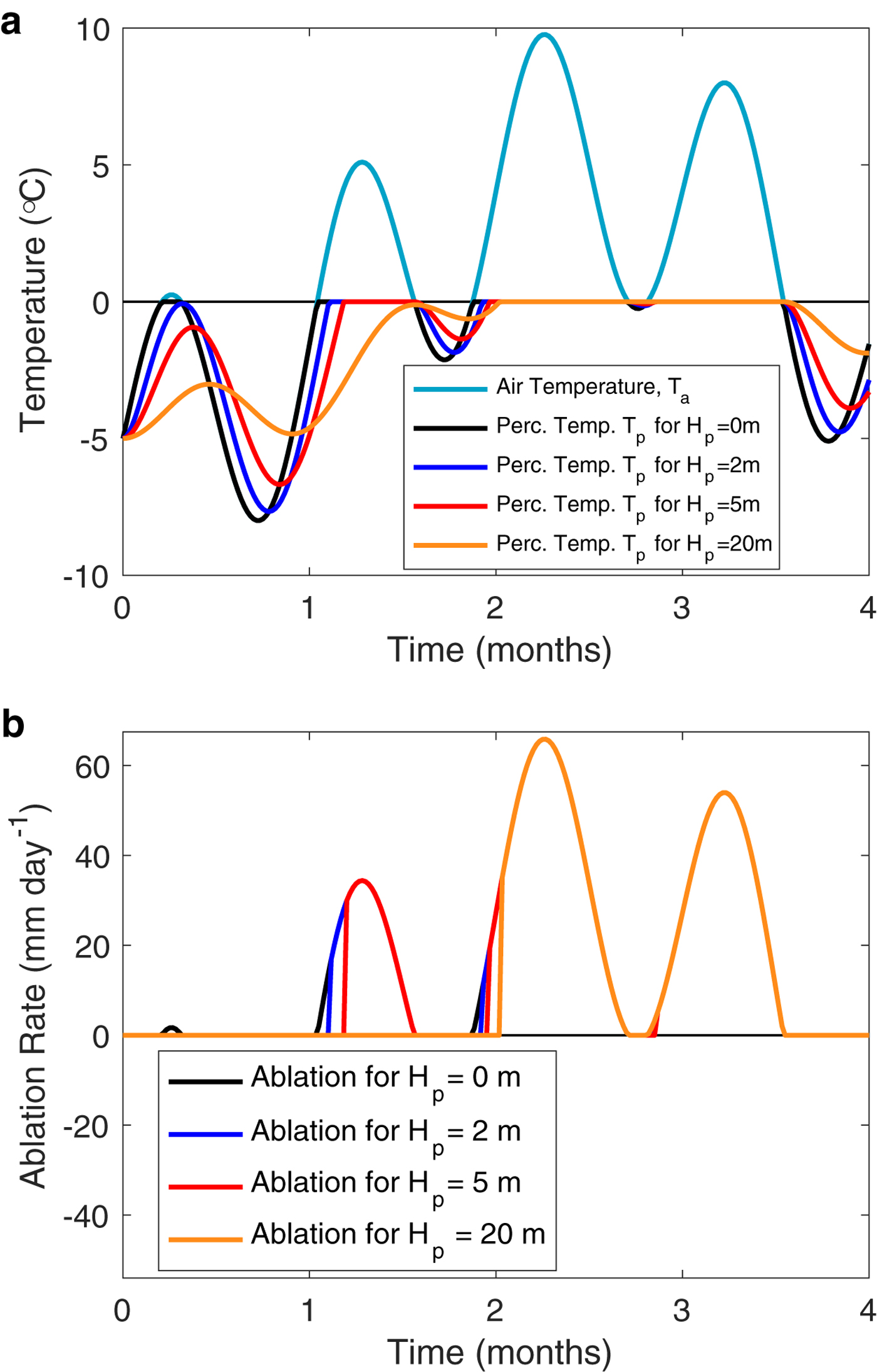
Fig. 2. Predictions of the model for idealized inputs. (a) Assumed air temperature T a(t) (cyan) and the predicted percolation layer temperatures T p(t) for four different assumptions for H p (0, 2, 5 and 20 m, corresponding to black, blue, red and orange lines). (b) Predicted ablation rate a(t) = −dz s/dt in mm day−1 for the four different H p as in panel (a) and with the same colors. Note that when predicted ablation is identical from different models, only line colors for larger H p appear.
3.2. Application to Qamanarssup Sermia
In this section, we apply our new model to observations of ablation and temperature at Qamanarssup Sermia in southwest Greenland (Braithwaite and Olesen, Reference Braithwaite, Olesen and Oerlemans1989; Olesen and Braithwaite, Reference Olesen, Braithwaite and Oerlemans1989; Braithwaite, Reference Braithwaite1995). Despite more than 20 years of new observations, the dataset of Braithwaite (Reference Braithwaite1995) still remains one of the more complete datasets for which observations of daily ablation rate and local air temperature are available. The primary dataset consists of daily ablation measurements averaged over three stakes and air temperature measurements made a few hundred meters away during the summers of 1980–86. At the Qamanarssup Sermia site (elevation 790 m a.s.l.), there is little to no snow, so that the ablation measurements are for ablation of ice. For some days, temperatures are reported but no ablation is reported and we assume that these days have ablation that is not significantly different from zero (daily ablation below 15 mm is rarely reported by Braithwaite, giving an estimate of uncertainties).
Our results from Section 3.1 show that the primary difference between our new model and the PDD model occur early in the melt season when the subsurface ice still has significant ‘cold content’ (Marks and others, Reference Marks, Domingo, Susong, Link and Garen1999) and when temperatures rise above 0 °C relatively quickly from significantly below zero temperatures. Of the 7 years of Braithwaite observations, only 1 year's data, that of 1986, has a long enough record at the beginning of the melt season, including times well before significant ablation occurs, to be useful for testing the new model. In 1986, measurements were made for more than 1 week without significantly nonzero ablation, and air temperatures averaged −3°C or colder for at least 20 days prior to warming above 0°C over the course of a few days. In all other years, observations did not begin early enough to capture the first significant period of above 0°C air temperatures, the time period for which the present model is expected to depart from the PDD model most significantly. We, therefore, test the model against the 1986 records, with daily ablation and daily mean air temperature measurements made from 1 June 1986 through 28 August 1986.
In order to have a continuation of air temperature measurements prior to the beginning of the Braithwaite observations, we use NOAA/NCEP Reanalysis daily mean air temperatures (Kalnay and others, Reference Kalnay1996) near Qamanarssup Sermia to estimate unmeasured air temperatures. Since the NOAA/NCEP temperatures are gridded quite coarsely (at 2.5° in latitude and longitude, or ~250 km), we take the four closest grid points and use the gridpoint with the best correlation with the Braithwaite measurements, i.e. at 62.5°N, 50°W (without any elevation correction). While this point is slightly farther from Qamanarssup Sermia (64.48°N, 49.48°W) than the nearest gridpoint (65°N, 50°W) of the NOAA dataset, it correlates with the Braithwaite measurements better and is therefore expected to better predict the temperatures at the site during other times as well.
Predictions for the percolation layer temperature T p(t) and ablation rate a(t) are shown in Figs 3a, b, respectively. Air temperature T a(t) is also shown in Figure 3a and both the measured ablation rates and PDD-estimated ablation rates are also shown in Figure 3b. Percolation layer temperature is initialized to −5°C on 1 January 1986 and the model is solved over the entire winter. Due to this long (5-month) spin-up time, predictions of summer ablation and percolation layer temperatures are not affected by the assumed initial condition. H p is estimated to be 5 m. This choice can be justified a posteriori based on the accuracy of the prediction, with values ranging between 4 and 6 m producing similar results. Percolation layer temperatures are found to be nonzero only in the early part of the Braithwaite observation period (prior to day 160) and predictions of ablation therefore track the PDD estimates of ablation exactly afterwards and thus for the vast majority of the data points. The only differences in the prediction of the new model appear during the initial few days of the Braithwaite observations. Despite this short period of time in which the model differs from the PDD model, it is clear that the new model improves upon the PDD model during this early time when zero ablation is observed. The model with H p = 5 m predicts the onset of melting on the correct day, whereas the PDD model predicts melting on early days for which no ablation is observed. (Note that increasing H p to 20 m would result in ablation not starting until day 170, later than observed.) Correlating the predicted ablation from both models with the observed ablation produces a correlation coefficient of 0.815 for the new model as compared with 0.803 for the PDD model, a modest gain in explanatory power. The improvement is modest because predicted percolation layer temperatures are 0°C for the majority of the observed time period.
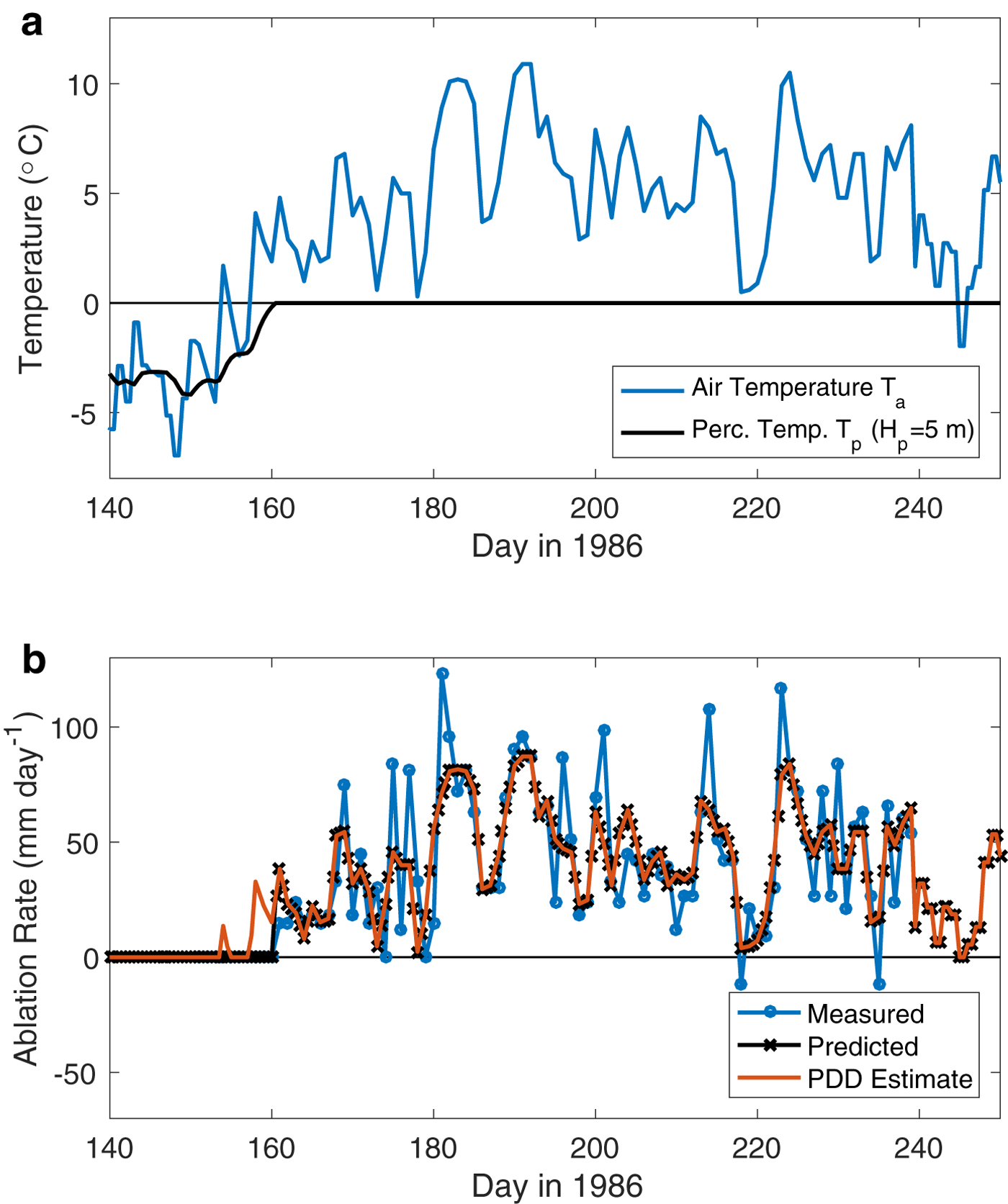
Fig. 3. Comparison of model predictions with observations at Qamanarssup Sermia during the melt season. (a) Air temperatures T a(t) (blue) observed by Braithwaite (Reference Braithwaite1995), continued into the early melt season using NOAA/NCEP Reanalysis surface air temperatures (Kalnay and others, Reference Kalnay1996), and modeled percolation layer temperature T p(t) (black). (b) Ablation rates measured by Braithwaite (blue), predicted by the present model (black) and using the traditional PDD estimate (orange).
As shown in Figure 4b, predictions of the new model are very different from those of the PDD model for the first 150 days of 1986 when no ablation measurements are available. The new model predicts only three days for which there is nonzero ablation whereas the PDD model predicts 28 days of nonzero ablation for the same time period. Thus, while the total ablation predicted over the full season is only 11% less, there is only 91 mm of ablation predicted over these first 150 days as compared with 530 mm for the PDD model, such that the first 500 mm of ablation occurs a full 47 days later than in the PDD model. While we have no independent measurements of ablation during this time period, the significantly negative percolation layer temperatures calculated during these times (see Fig. 4a) suggest that any melt produced during this time would quickly refreeze to warm the percolation layer. Even if the estimated H p were smaller during this time, one would expect H p to be at least ~1 m (as discussed previously) and predicted ablation would still be significantly less than PDD estimates over this time period. We note that ‘enhanced’ PDD models that use observed radiation along with air temperature to empirically estimate ablation (e.g. Pellicciotti and others, Reference Pellicciotti2005) may also predict less early spring ablation, but for a different physical reason than proposed here.

Fig. 4. Comparison of model predictions at Qamanarssup Sermia over the full year. (a) Air temperatures T a(t) (blue) observed by Braithwaite (Reference Braithwaite1995), continued using NOAA/NCEP Reanalysis surface air temperatures (Kalnay and others, Reference Kalnay1996) and modeled percolation layer temperature T p(t) (black). (b) Ablation rates predicted by the present model (black) and using the traditional PDD estimate (orange).
The most important implication of the new model is that ablation is expected to be significantly lower for the same temperature early in the melt season as compared with later. The predicted date of the beginning of ablation is thus expected to be significantly later than estimates from a PDD model. This delay of melting may, in turn, have important implications on whether subglacial meltwater drainage lubricates the ice sheet or not (Schoof, Reference Schoof2010). Furthermore, due to the delay inherent in the diffusion of heat, there is a natural hysteresis predicted in ablation rate versus air temperature, which also makes ablation nonlinearly related with air temperature. This general conclusion agrees with other recent findings that ablation rates (and their standard deviations) may not be linear with temperature (Wake and Marshall, Reference Wake and Marshall2015).
3.3. Application to PROMICE data across the Greenland ice sheet
Another dataset for which in situ ablation measurements were made is the PROMICE (Programme for Monitoring of the Greenland ice sheet) dataset (Machguth and others, Reference Machguth2016b; Van As and others, Reference Van As2017), which includes ablation measurements at 22 automatic weather stations across the Greenland ice sheet for multiple years. While the ablation data are not of uniform quality, including many times when ablation is not reported and other times for which ablation may be misreported due to the automated nature of the recordings (Fausto and others, Reference Fausto, Van As, Ahlstrom and Citterio2012), there are a number of sites for which full years of uninterrupted, high-quality ablation measurements are available. We validate our model with ablation measurements at the five PROMICE sites for which multi-year nearly continuous daily ablation measurements are available (using ablation from channel AblationPressureTransducer of the PROMICE flat files as described in Van As and others, Reference Van As2017). Comparisons of the measured ablation, PDD estimates and our model estimates are shown in Figure 5 along with predicted percolation layer temperatures as in Figure 3. For each site, degree-day factors were first estimated by fitting the PDD model to the ablation measurements (see label β in each panel of Fig. 5). These degree-day factors were then fixed and percolation layer thickness were estimated by fitting the new model to all of the ablation measurements at each site (see labels of H p in each panel of Fig. 5). To model the 12 years of data shown in Figure 5, we ran the model for 40 years (including years not shown) at 12-h temporal resolution, which took 6 s on a modern (3.1 GHz) laptop computer, suggesting that computational time is reasonable for the results shown in Figure 5.
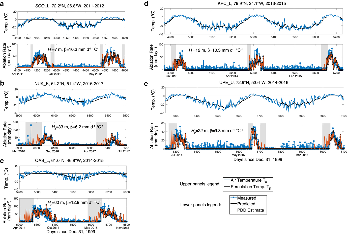
Fig. 5. Comparison of model predictions with observations at PROMICE sites. Data are shown for two consecutive seasons for stations (a) SCO_L, (b) NUK_K and (c) QAS_L, and for three consecutive seasons for stations (d) KPC_L and (e) UPE_U. In each panel, upper subpanels show observed air temperatures T a(t) (blue) and modeled percolation layer temperature T p(t) (black) whereas lower subpanels show ablation rates as measured by PROMICE pressure transducers (blue), predicted by the present model (black) and using the traditional PDD estimate (orange). Light gray shading is used to highlight time periods for which the present model improves upon the PDD model. Values of H p and degree-day factor β used for the modeling are given in each panel. For a map showing PROMICE site locations, see Van As and others (Reference Van As2017).
As can be observed in Figure 5, ablation estimates at each site and each season are improved with the current model as compared with the PDD model, with shaded areas in Figure 5 highlighting time periods with the most significant improvement. As with the Braithwaite data, the improvements are mostly in the early parts of the melt season. Counting the number of days for which above 10 mm day−1 is predicted by the PDD model prior to any predicted ablation with the current model, for example, we find 4 such days for the 2012 season of SCO_L, 33 days for 2016 NUK_K, 38 for 2014 QAS_L, 9 days for 2015 KPC_L and 15 days for 2016 UPE_U. We note that in the ablation comparisons, the nonzero ablation reported during winter time periods may be suspect and may better reflect measurement errors at each site. Interestingly, there is a wide range of percolation layer thicknesses required to fit the data, with H p ranging from 7 m at SCO_L, 12 m at KPC_L, 22 m at UPE_U and 33 m at NUK_K to 60 m at QAS_L. These large percolation layer thicknesses and associated large delays in ablation relative to PDD model estimates underscore the need to incorporate a model like the one proposed to correctly estimate ablation during the early melt season. While the spatial variability in percolation layer thicknesses required has not been verified in situ, the large range of values suggests that it will be important to understand the spatial and temporal variability of the model parameters (primarily H p and k), including differences for snow versus ice.
Finally, we note that the 2017 melt season at NUK_K (see Fig. 5b) is the only season (of the 12 seasons modeled) for which our new model does not well capture the beginning of ablation as measured by the PROMICE pressure transducers. Tests show that even allowing for a larger H p compared with that which best fits the 2016 data does not result in a good match of the 2017 NUK_K data. We suggest that the pressure transducer measurements for that one season are not reliable despite passing our quality control metrics, primarily due to time periods for which no ablation is reported (which is reported differently than ablation measured to be zero). It should be noted that many of the other PROMICE stations had similar issues, but all other seasons were rejected from our modeling test due to other data quality criteria including lack of continuity of measurements.
4. CONCLUSIONS
We have presented a new simplified model in which observations of surface air temperature can be used to construct a physically meaningful estimate of ice ablation rates from the surface of an ice sheet or glacier. This model only has one additional parameter, the percolation layer thickness, as compared with the PDD model and is therefore simple to use. While it is certainly not expected to be as accurate as a full energy-balance model, the ability to use the model in essentially any circumstance in which the PDD model can be used, while having a sound physical basis that the PDD model lacks, makes the new model particularly attractive for use across a wide range of applications and particularly in cases where empirical calibration is difficult. The new model is found to simplify exactly to the PDD model if either the percolation layer thickness is infinitesimally thin or if the glacier is purely temperate (0 °C throughout), though an infinitesimally thin percolation layer is never expected to exist in reality. Application of the model to Greenland ice sheet data suggests the model is more accurate than the PDD model, with predicted differences with respect to the PDD model being largest in the early melt season. The model may also apply to other glaciers worldwide, though we have not yet evaluated how much it improves upon the PDD model in other circumstances and we suggest that the model should be tested in these other regions. Nonetheless, we suggest that researchers currently using the PDD model to predict ablation rates could benefit significantly from using our modest modification to the PDD model and would allow them to more accurately predict both the date of first melt as well as the amount of melt at the beginning of the melt season.
SUPPLEMENTARY MATERIAL
The supplementary material for this article can be found at https://doi.org/10.1017/jog.2018.55
ACKNOWLEDGEMENTS
We thank three anonymous reviewers for their constructive comments. This work was partly supported by NSF grant OPP-1735715.


 Open access