Bathymetry and surface features

We used sonar sounding from a small boat to determine the bathymetry in the recently deglaciated fjord. Our data were quite dense in the near-terminus environment, and they show that the steep-walled fjord has a maximum depth of ∼270 m below sea level. A terminal moraine exists 2 km down-fjord of the present terminus, marking the most recent (1962–94) position of stability. There the water depth shallows to about 190 m. Given the highly resistant surrounding bedrock, formation of such a submarine moraine is likely a much slower process than is typical for many other tidewater glaciers in Alaska, which generally erode soft sedimentary or metamorphic rocks (Reference Hunter, Powell and LawsonHunter and others, 1996).

The terminus is completely grounded, but the majority of the terminal ice lies below sea level. With an average ice-cliff height of 40–60 m above the sea surface (as determined by helicopter-borne differential global positioning system (GPS) measurements and terrestrial surveying (accuracy 1–2 m)), the terminus is currently only 20–25 m above flotation. The glacier center line is shifted approximately 150 m south of the deepest part of the channel (Fig. 2a). The nearterminus surface topography is steep, with surface slopes on the order of 10°. Heavy crevassing dominates the lower 8 km of the glacier, with the last 4 km composed mainly of seracs and ice pinnacles.

Fig. 2. (a) Glacier terminus and fjord bathymetry as measured in 1999, looking down-fjord. (b) Location of the transverse markers (hexagons). A gap exists between the ice and margin, as shown. The arrow marks the location of the cross-section shown in (a); asterisks denote replacement markers.

Motion

Horizontal and vertical ice motion were monitored for 37 days (2 May–4 June and 26–30 August) at several markers. We used optical survey methods and tetrahedral markers placed on seracs. Over the course of the study, we deployed a total of 18 markers 0–7 km from the terminus. Thirteen of these markers were placed near the longitudinal center line of the glacier (labeled A–G, plus Bend and Gate in Fig. 1b). The remaining five were set on a transverse profile across the width of the terminus (labeled T1–T5 in Fig. 2b); these were surveyed for only 2 days (Fig. 3). Due to serac instability and calving losses, some markers were periodically reset; new positions were chosen as close to the initial marker positions as possible in order to investigate the temporal changes in motion at a given point in space (i.e. within an Eulerian reference frame). Replacement markers are labeled with an asterisk (e.g. B^*). A longitudinal coordinate system ξ ∊ [0, 9 km] was defined with the origin (ξ = 0) located just up-glacier from Gate (Fig. 1b), where the glacier enters a well-defined constriction, and is positive towards the terminus. ξ = 0 is near the average 1990s equilibrium line, ξ = 7 marks the May 1999 terminus position and ξ = 9 the 1962–94 position.

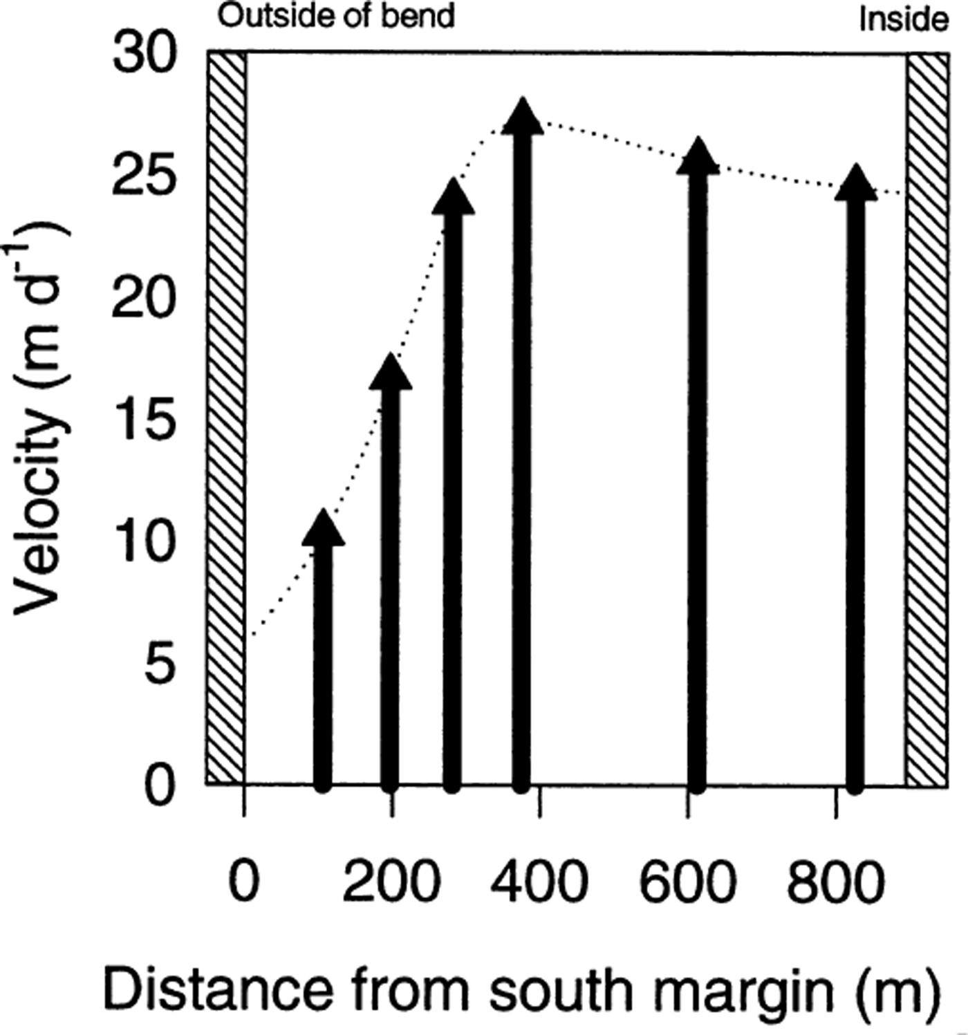
Fig 3. Transverse velocity profile at the terminus. The maximum ice velocity is shifted towards the outside of the bend by about 80 m. Note that sliding occurs even at the margins.

As we were interested in identifying any tidal forcing of glacier speed, we attempted motion surveys at intervals of a few hours in order to satisfy the Nyquist sampling criteria (a sampling interval less than or equal to 1/(twice the frequency of interest); Reference GodinGodin, 1972). For a semi-diurnal cycle, this requires sampling at least four times per day. When possible, we surveyed at 2–3 hour intervals, with a 3–6 hour gap at night. Therefore, our surveys generally satisfy the sampling criteria, but the sampling interval was not constant and there were data gaps.

The weather during May 1999 was unseasonably poor, and markers were sometimes obscured by clouds or precipitation during a survey. However, the resulting time series of motion are relatively complete, as can be seen in Figure 4a. The estimated errors in the surveyed positions range from ±3 cm in good conditions to ±6 cm in poor surveying conditions. Over 3 hour time intervals these correspond to errors in velocity of ±0.34 and ±0.68 m d⁻¹, respectively. Additional errors were occasionally introduced by marker tilt or rotation. The average error in vertical position is estimated to be ±5 cm.

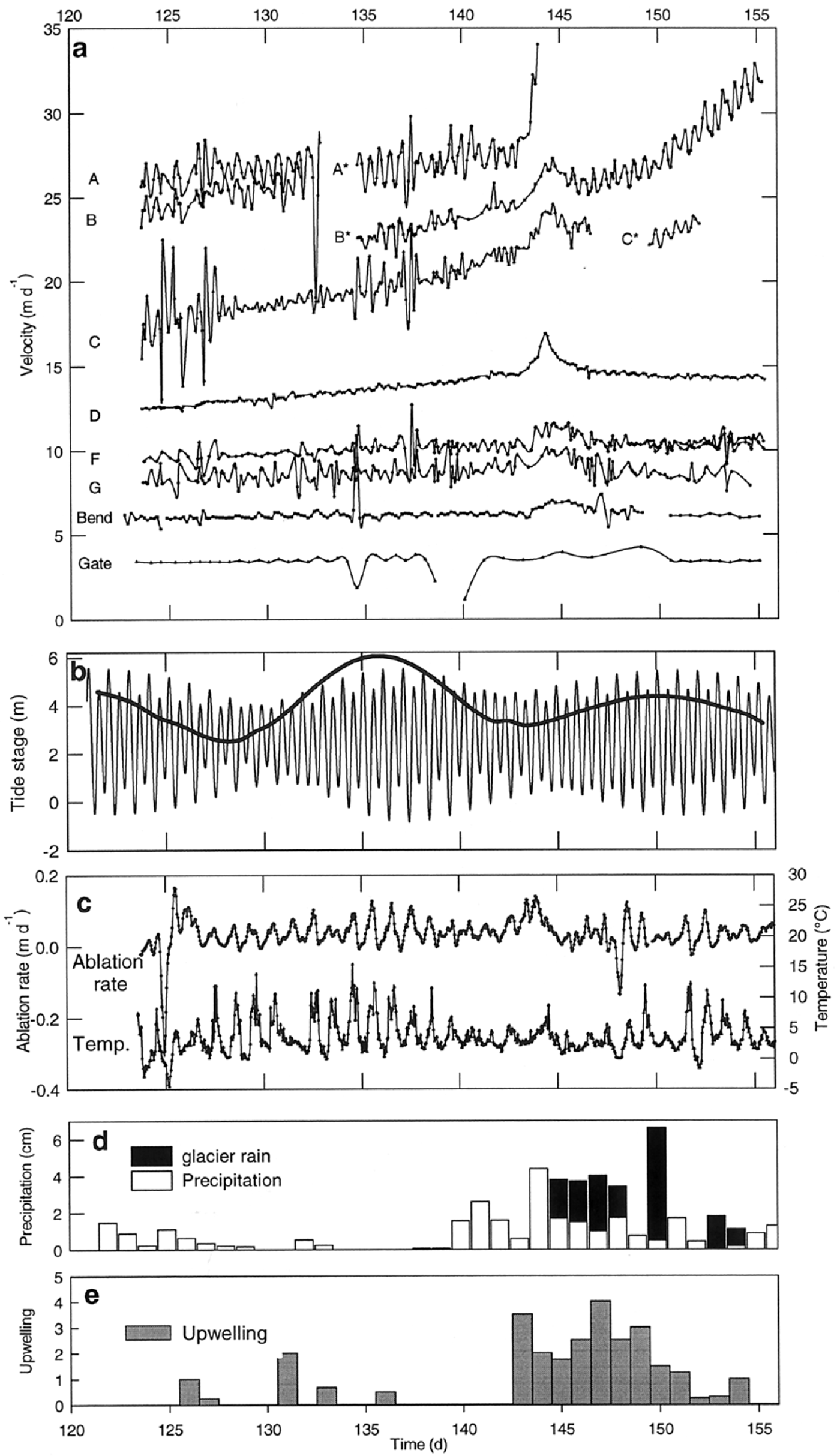
Fig. 4. (a) Velocity of each marker. (b) Predicted tide (thin line) and tidal amplitude (bold line). (c) Ablation rate and temperature as measured on an adjacent glacier. (d) Precipitation at Petersburg Airport, and, when available, local precipitation. (e) Upwelling at the terminus.

Further upstream at Bend and Gate (Fig. 1b), we deployed dual-frequency GPS receivers, with position data six and two times daily, respectively, for the duration of the study. Postprocessing of these data against a nearby base station (“Lake”, Fig. 1b) gave a positional accuracy of about 3 cm; rotation of the markers as crevasses opened may have caused some degradation of this accuracy. A few gaps exist in this otherwise continuous record because of power losses.

Tide

Complete knowledge of the ocean tide at the glacier terminus is critical to our analyses of velocity and calving. The closest continuously operating tide gauge was located in Ketchikan, Alaska, >100 km from the glacier. To more accurately determine the tide near the glacier we obtained U.S. National Oceanic and Atmospheric Administration (NOAA) water-level data collected in LeConte Bay during spring 1997 (http://www.co-ops.nos.noaa.gov/data_res.html). We also installed our own tide gauge in the bay during August 1999. Using these data, we were able to prescribe the local tide at any time during our study, as described below. The tide in LeConte Bay (Fig. 4b) has a strong semi-diurnal component, with two highs and lows of unequal magnitude each day. Peak-to-peak amplitude varies from about 2.5 to 6 m. In what follows we refer to the daily “tidal amplitude”, which we define to be the range between the average of the two high tides and the two low tides each day.

Other observations

Hourly air temperature (±0.4°C) and ice ablation (±1 cm) were measured using a thermistor probe, sonic ranger and data logger situated on a tributary glacier about 3 km from the terminus and 530 m a.s.l. The ablation rate (time derivative of the ablation data; Fig. 4c) exhibits clear diurnal variations, even though variable weather and long-duration rain events introduce large variability in the timing (±0.2 days) and magnitude of the peak ablation rate. Thus the ablation rate has a broad spectral peak, centered around 1 cycle d⁻¹. Negative values represent snowfall events.

Daily precipitation was measured by the U.S. National Weather Service at Petersburg Airport. We also measured precipitation for 9 days (days 145–154) at a temporary gauge near the terminus. The two records generally follow similar trends, but the magnitude of the precipitation at the glacier was often twice that measured in Petersburg (Fig. 4d). However, at times the precipitation differed markedly; the rain event recorded in Petersburg on day 151 occurred 1 day earlier at the terminus.

Water discharge from a tidewater glacier is difficult to monitor, but it plays an important role in basal hydrology and glacier motion. As a proxy for discharge, we made qualitative estimates of upwelling at the terminus by observing the timing and magnitude (0–5) of silt-laden fresh-water plumes in the fjord, just downstream of the terminus (Fig. 4e). Upwelling plumes were easily recognizable as they would drive icebergs and brash ice away from the terminus, and a strong upwelling event (magnitude 5) would create whitecaps in the forebay. An absence of upwelling (magnitude 0) left the terminus region packed with ice.

Flow around a bend

As ice approaches the terminus of LeConte Glacier, it flows around a sharp bend. There the center-line radius of curvature is about 1.1 km, while the glacier is only 1 km wide. This causes a change in flow direction of >90° (Fig. 1b). The transverse velocity profile near the end of this bend shows that the flow maximum is shifted outward by about 80 m from the glacier center line (Fig. 3). Theory describing ice flow in a curving channel (Reference Echelmeyer and KambEchelmeyer and Kamb, 1987) accurately predicts this outward shift, but the details of the velocity profile and those of the theoretical one differ because basal (and marginal) motion dominates the actual flow. According to this theory, the surface slope should vary across the glacier, with maximum slope on the inside of the bend. Such a variation in slope is observed.

Strain rate

As ice approaches the terminus, it is subject to large longitudinal gradients in velocity (up to 6 a⁻¹) and in strain rate (Fig. 5). These strain rates are extremely large, being about an order of magnitude greater than those observed in the past on Columbia Glacier (Reference Venteris, Whillans and van der VeenVenteris and others, 1997). The strain rate reaches a maximum value about 200 m up-glacier from the terminus; it then drops an order of magnitude in the last 200 m to the terminus. This maximum occurs about one cross-sectional average ice thickness back from the terminus. These high strain rates cause heavy crevassing, as well as thinning in the terminus region. The recent thickness change at the terminus is known from repeat airborne profiles in 1996 and 2000; we estimate that thinning caused by longitudinal stretching alone is 19 m a⁻¹, or about 60% of the measured thinning rate. As noted above, the motion of the markers within such an extending flow regime leads to an apparent temporal increase in speed; this is a spatial rather than a temporal effect.

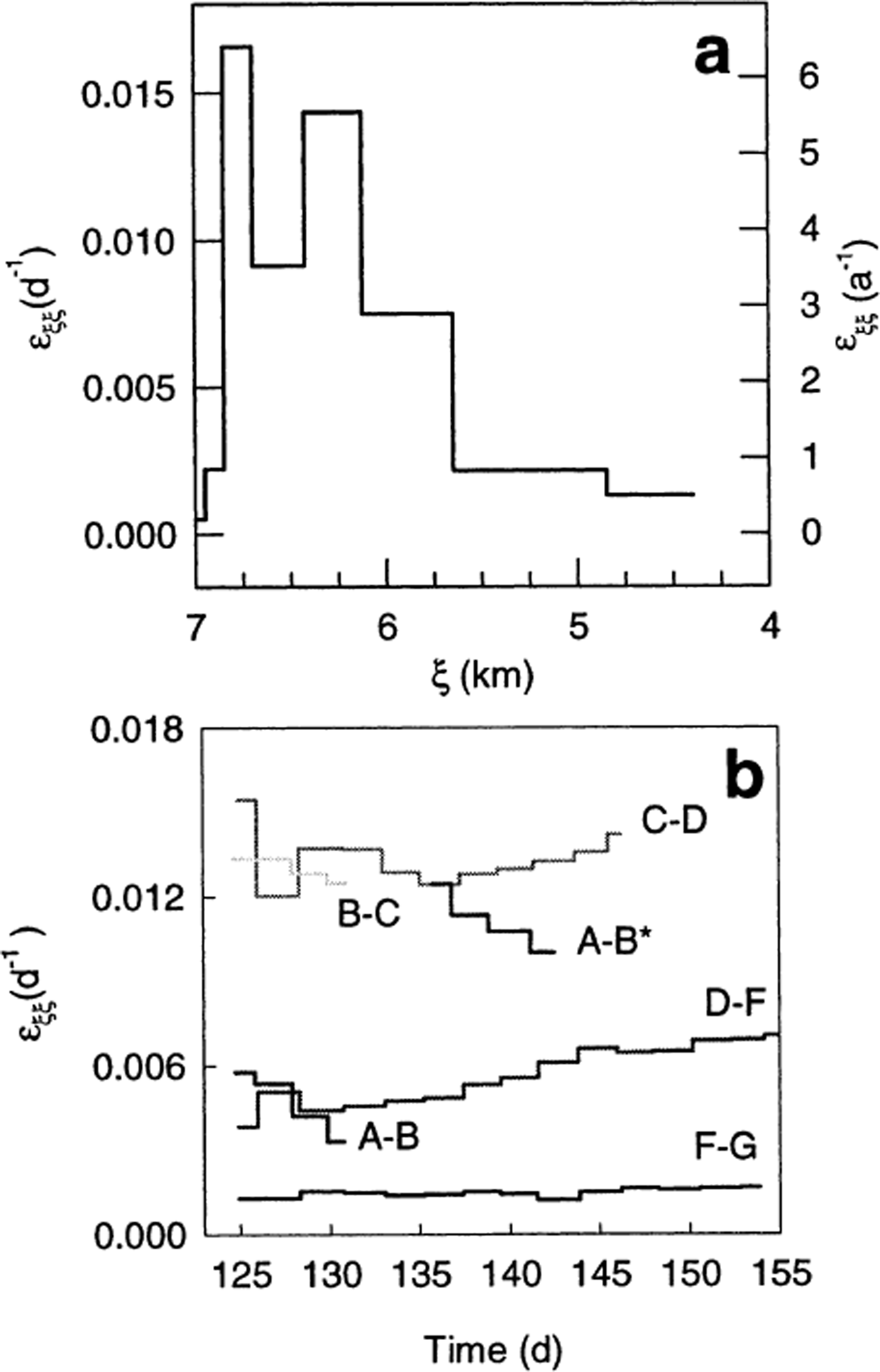
Fig. 5. (a) Longitudinal strain rate plotted as a function of ξ; extension is positive, (b) Longitudinal strain rate between markers as a function of time. At no time during the study was any part of the terminus region under longitudinal compression.

Seasonal variations in speed

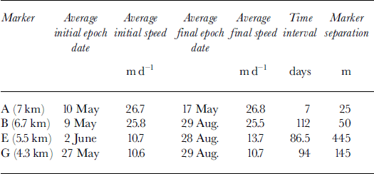
Table 1 gives a comparison of velocity measurements made at similar locations on the glacier surface at different times of the year. These comparisons were made between markers that were located < 2 m apart along the flow direction to minimize errors due to the large longitudinal strain rates. The dates given in this table are the mid-times of the early-season velocity epoch (column 2) and of the later velocity epoch used in the comparison (column 4), while column 6 is the length of time over which the comparison is made. Columns 3 and 5 are the two velocities that are to be compared. The distances in the last column of Table 1 are the spatial separations of the markers between the two measurement epochs, as measured transverse to the flow direction. Large transverse separations in this column will introduce errors in our assumed temporal comparisons because of transverse variations in speed, but these are likely to be small as the flow is plug-like. Marker A shows no change in speed from pre-melt conditions (and no water input at the surface) into the early melt season. The other comparisons span a 3–4 month interval from early May to the end of August. The early part of this interval was characterized by precipitation as snow and little melt on the glacier; the middle spans the entire melt season; and at the end, new snow was accumulating on the glacier as low as Gate (700 m elevation). Over this interval, the glacier speed at these three locations was nearly constant; any differences are likely accounted for by the transverse position of the markers (especially marker E). Additional data come from the continuous GPS record obtained at Gate, which shows short-term variations but no seasonal change in speed over the same >100 day interval (Fig. 6). These results indicate that there is no change in speed over the lower 7 km of the glacier from late in the winter season through the entire melt season. Because this interval spans the transition from no surface input of water to the glacier system to a time of substantial water input, these results support the idea that there is little or no seasonal variation in speed on lower LeConte Glacier. Of course, it is possible to construct scenarios of summertime speed oscillations that would produce the observed lack of seasonal variation within our sampling scheme, but these scenarios are unrealistic.

Fig. 6. Surface velocity at Gate. No seasonal changes are apparent.

Table 1. Seasonal changes in speed. The velocities for markers moving along similar flowpaths at different times are shown. Marker separation distances are transverse to flow

Harmonic analysis of the tide

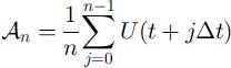
The standard techniques of “harmonic analysis” (Reference GodinGodin, 1972; Reference ForemanForeman, 1993) were used to analyze the local tide and, subsequently, the ice-speed data. In this analysis we assume that a time series can be partially represented by a sum of discrete sinusoids, each with a prescribed frequency, ω_i (rad h⁻¹), as determined by tidal forces, but with unknown amplitude, A_i, and phase φ_i . That is:

(1)

where is the tide (or later the ice speed), t is the time in hours, M is the mean of , and the subscript i ranges over the N constituents assumed to make up the time series. Nonlinear least squares is then used to solve for the unknown amplitude and phase of each constituent. We also calculated the reduction of variance (ROV) in a stepwise fashion as each constituent is added to the analysis. This allows us to assess the relative strength of each constituent, and the chi-squared test (χ ²) was used to determine the statistical significance of the predicted series. A residual time series, equal to the input series minus the N-component predicted series, was also calculated for later analyses.

The primary tidal constituents are either semi-diurnal or diurnal. Notation for these constituents consists of a letter representing the source (lunar, solar), followed by a subscript delineating the approximate frequency per day (diurnal = 1, semi-diurnal = 2; Reference GodinGodin, 1972). For example, M ₂ is the principal lunar semi-diurnal constituent.

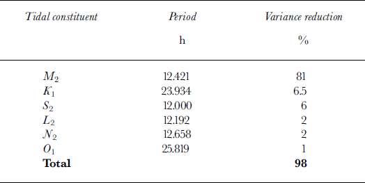
We used the 1997 NOAA tide observations from LeConte Bay to solve for the amplitude and phase of the dominant tidal constituents. This solution was then checked against our 1999 tidal measurements, using a prediction via Equation (1). The six strongest constituents of the LeConte Bay tide are listed in order of decreasing importance in Table 2. These constituents determined ∼98% of the variance in the tide signal. The semi-diurnal constituent M ₂ dominates the tide (81% ROV), followed by the lunar diurnal constituent, K ₁. The tide is relatively free of complicated shallow-water, overtide constituents at higher frequencies.

Table 2. LeConte Bay tide: tidal constituents (Reference GodinGodin, 1972), their periods and strength in the local tide

Using Equation (1) and the amplitude and phase for these six constituents, we can predict the tide at any time of interest, in particular during our survey in 1999 (Fig. 4b). The estimated accuracy is 0.25 m, with few or no phase discrepancies, except during extremes in atmospheric pressure.

Short-term variations in horizontal motion

Here we describe the methods and results of our analyses of horizontal speed, U(t), over tidal to several-day time periods.

Signal filtering

Prior to the analysis, we detrended, smoothed and filtered the speed series displayed in Figure 4a. An Eulerian reference frame was approximated by removing the effects of the large longitudinal velocity gradients (Fig. 5). Cubic splines were fit to these data, and these were sampled at 3 hour intervals (our nominal surveying interval). These series were then subjected to a low-pass filter with a cut-off period of 24 hours in order to isolate that portion of the signal at lower than tidal frequencies. The filter used was , where

(2)

(Reference GodinGodin 1972, p.65). U is the ice speed, Δt is our sampling interval (3 hours), and n = 8. Now isolated, the low-frequency part of the signal was subtracted from the splined interpolant, leaving the high-frequency portion of the signal, U _highfreq.

(3)

We describe the low- and high-frequency parts of the signal in turn.

Low-frequency variations

The low-frequency time series, , for each marker are shown in Figure 7. The most prominent feature of these series is the speed-up event centered around day 144.5, which lasted about 3 days and had an amplitude of 5–13% of the mean speed at each marker. The onset, duration, and time of peak speed are similar for each of the markers, with a variance of < 0.5 day in their timing.

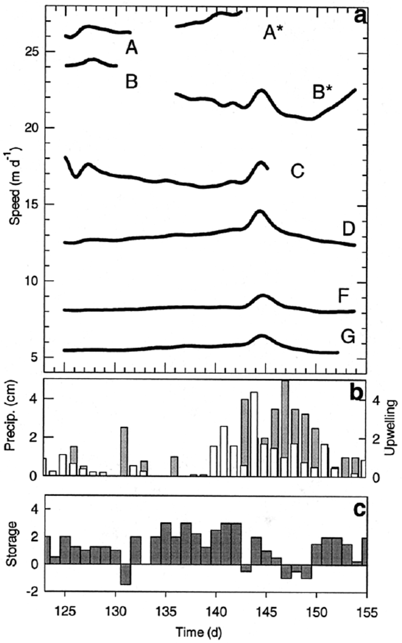
Fig. 7. (a) Low-frequency speeds for markers A–G; (b) precipitation (white) and upwelling (grey); and (c) a qualitative storage index.

A correlation (correlation coefficient, C = 0.54−0.66) with a phase lag of +1.0 day exists between the low-frequency speeds and excessive water input provided by heavy precipitation, such that precipitation events precede the maximum velocity. At some locations the speed decreased to a level that was lower than before the speed-up event (e.g. markers B^*, D, G).

To investigate possible effects of water storage, we estimate a crude water-storage index (Fig. 8c). This index was compiled by differencing qualitative magnitudes of water input and output each day. Inputs and output were included in the index only when they were above “base” levels. Water input included any recorded precipitation and any surface melting in excess of the lowest maximum daily melt rate. Any observable upwelling (Fig. 8b) was considered to be above the base-level discharge. The velocity peak around day 144 is centered on an abrupt change in the water-storage index. However, the largest peaks in storage index did not coincide with velocity peaks.

Fig. 8. Measured high-frequency horizontal speed (solid line) and the harmonic analysis prediction (dotted line and triangles).

Semi-diurnal variations

We applied harmonic analysis to the high-frequency time series, U _highfreq, following Equation (1). These results are presented in Table 3, where the total reduction of variance and the ROV for the semi-diurnal M ₂ constituent alone are given, as well as the amplitude and phase for each constituent for each marker. Markers A/A^* and B^* demonstrate the best overall ROV, and there is an approximate up-glacier decay in the overall ROV. Near the terminus (B^*, Fig. 8), the predicted series matches the observations quite well (χ ² for markers A/A^* and B^* yields < 1% probability of a random fit). Even in these cases, however, the ROV is < 50%, indicating that the velocity fluctuations are not completely tidal in nature. The upstream markers have a poorer fit (e.g. F in Fig. 8; see also Reference O’NeelO’Neel, 2000), and the probability of a random fit is on the order of 50%. Marker C has an abnormally noisy record.

Table 3. Harmonic analysis of horizontal velocity: amplitude (A) and phase (φ) relations for each marker and the tide using the six strongest tidal constituents. The total ROV and the M₂ ROV are given in parentheses

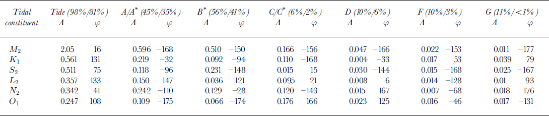
The results in Table 3 show that, as in the case of the tide, most of the speed fluctuations are semi-diurnal (M ₂). The other constituents in the speed are poorly resolved, as their signal is either too weak or contaminated by other forcings (also noted on Columbia Glacier by Reference Walters and DunlapWalters and Dunlap, 1987). Such contamination from non-tidal forcings is illustrated by abrupt changes in phase between constituents of similar frequency (Table 3), rather than a smooth response (Reference Zettler and MunkZettler and Munk, 1975). We therefore take the M ₂ response given in Table 3 to represent the effects of the tide on velocity at each marker.

The M ₂ phase angle for the tide is 16°, and the average M ₂ phase angle for markers A/A^* and B^* is about −160°. Thus, the phase difference between the two is 176°. Minimum speed occurs at peak tide, with virtually no phase lag.

Statistical analysis shows that the amplitude of M ₂ given in Table 3 is well resolved. It thus provides a means for studying the up-glacier propagation of tidal forcing through its amplitude admittance. We define the M ₂ admittance, as the ratio of the amplitude of the M ₂ speed variation to the amplitude of M ₂ in the tide:

(4)

There is an exponential decay in with distance up-glacier from the terminus (Fig. 9). This decay has a characteristic damping length (damping to 1/e of peak value) equal to 0.5 km, or about 1.2 times the center-line ice thickness at the terminus.

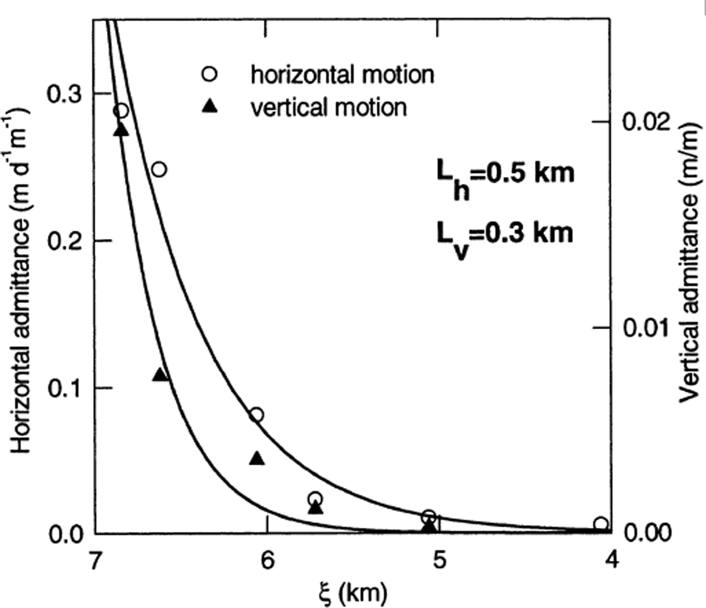
Fig. 9. Horizontal and vertical M₂ admittances (circles and triangles, respectively).

Diurnal variations

Diurnal cycles exist in both temperature and ablation rate. These cycles likely influence water input to the glacier system, and therefore may affect glacier speed. However, resolving such forcing is difficult because the tide also contains some diurnal constituents, albeit with low energy. Separation is especially difficult because of the broad width of the diurnal melt peak, which is indicative of variable weather conditions.

In an effort to separate these two signals, we assume that U _highfreq is a linear combination of two terms: U _tide, which accounts for motion driven by the tide, and U _melt, which represents meltwater-forced motion plus noise. Then

(5)

We then assume that U _tide can be prescribed by the M ₂ admittance as applied to the other constituents by an admittance transfer function:

(6)

Here is the expected phase angle for the ith constituent, obtained by shifting the ith tidal phase by 176°, as found for M ₂. Thus, we assume that the relative admittance of each of the six constituents is equal to the well-resolved M ₂ admittance. Tests with synthetic data have shown that this admittance transfer function (Equation (6)) is effective for separating a melt signal from a tidal one (Reference O’NeelO’Neel, 2000).

Following Equation (5), this admittance transfer function was subtracted from the high-frequency time series to obtain U _melt. These results show that melt-driven variations in horizontal motion are best developed upstream at markers D through Bend (Fig. 9; Reference O’NeelO’Neel, 2000), but they exist to some degree at most markers.

The average amplitudes of the melt-forced variations in speed were estimated for each U _melt series. A step change in the peak-to-peak amplitude occurs between markers C and D; A–C have amplitudes of ∼50 cm d⁻¹, while markers upstream have smaller amplitude variations of only ∼20 cm d⁻¹. However, the upper markers have less “noise” due to tidal forcing, so diurnal fluctuations are better resolved there.

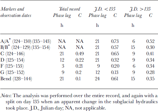
We used cross-correlation to identify the lag between surface ablation and ice speed. In all cases, the ablation-rate peaks precede increases in speed (Table 4). The statistical significance of the correlations was small when calculated over the entire interval; this indicates that the phase lag between the two variables is not constant. However, by splitting the time series into two intervals (days 124–135 and 135–154), the correlations between the variables for each interval and for each marker are greatly improved (Table 4). Day 135 thus marks a change in the response time of the speed to melt forcing; the average response time is reduced from 23 hours to 10 hours. Prior to day 135, the phase lag generally increases up-glacier, but after day 135 it is more variable, exhibiting no obvious trends.

Table 4. Cross-correlation (correlation coefficient C) between U _melt and ablation rate

Short-term variations in vertical motion

We next consider the vertical position, z(t), of each marker over the same time-scales as those discussed for horizontal speed, using the same analysis methods. For each marker, downslope movement was removed by subtracting a quadratic representation of the local glacier surface from the z(t) series, as determined by airborne surface profiling.

Low-frequency vertical variations

The low-frequency vertical displacement signals (Fig. 10) do not show a consistent pattern at the different markers; some of this may be due to the detrending applied to the data. The upstream markers (D, F, G) show an uplift event centered on about day 145 corresponding to the precipitation-related speed-up event shown in Figure 7; this is not observed at the near-terminus markers. After heavy rain, the glacier surface at D–G is uplifted; it then drops upon the initiation of up-welling. There was no longitudinal compression during these vertical motion events.

Fig. 10. Low-frequency vertical position for each marker. Precipitation (white) and upwelling (black) are shown in lower panel.

Fluctuations in vertical position at marker A/A^* are approximately in phase with the tidal amplitude; minimum surface elevation coincides with minimum tidal amplitude. Vertical motion at markers B and C shows no correlation with either the tidal amplitude or precipitation.

High-frequency vertical variations

Harmonic analysis of z _highfreq(t) shows that semi-diurnal tidal forcing of surface elevation exists only at the markers closest to the terminus (e.g. A/A^*, Fig. 11). However, even though this figure appears to show a strong semi-diurnal signal at A/A^*, the ROV for the M ₂ component is small there, and even smaller for B^* (Table 5). The peak-to-peak amplitude of the M ₂ variation at A/A^* is on the order of 13–18 cm, with a phase lag of about 90°, such that the maximum surface elevation follows the high tide by ∼3 hours. This implies that the maximum uplift rate (dz/dt) occurs at high tide. The up-glacier decay of the semi-diurnal fluctuations in z is more rapid than the horizontal M ₂ motion (L _v = 0.3 km; Fig. 9). Because the semi-diurnal tidal constituent M ₂ does not dominate the signal, the admittance transfer function (Equation (6)) cannot be applied to further analysis of z(t).

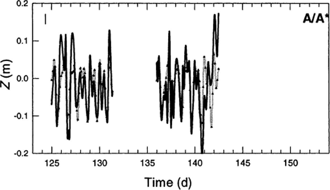
Fig. 11. z _highfreq formarkerA/A^* (solid line) and the harmonic analysis prediction (dotted line and triangles). A typical error bar is shown in the upper left. This semi-diurnal forcing exists only near the terminus and is rapidly damped up-glacier.

Table 5. Harmonic analysis of vertical position. The variance reduction is shown for the M ₂ constituent, as well as the combined reduction for diurnal constituents K₁ and O₁

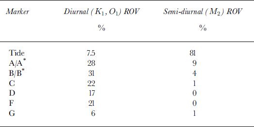
For the vertical position of markers A–F the variance reduction due to the diurnal constituents K ₁ and O ₁ is significantly greater than the ROV in the tide for these same constituents (Table 5). The peak-to-peak amplitude of these diurnal variations is fairly constant (8–12 cm) between the markers, which we feel is above our level of measurement uncertainty. These results suggest that the diurnal fluctuations in uplift are related to diurnal meltwater production, and not K ₁ and O ₁ tidal forcing.

Semi-diurnal variations

Ice speed on LeConte Glacier is 180° out of phase from the tidal stage. A 1.5% variation in sea level (∼3.0 m of 171 m mean depth) causes a 5.5% fluctuation in speed (∼1.5 out of 27 m d⁻¹ mean speed, marker A/A^*). Equivalently, this may be expressed as 0.5 m d⁻¹ per m of tide. On Columbia Glacier, Reference Meier and PostMeier and Post (1987) reported a 4% variation in speed caused by a 1% fluctuation in tide, or 0.2 m d⁻¹ per m of tide. Reference Walters and DunlapWalters and Dunlap (1987) also found that the speed at Columbia Glacier was nearly 180° out of phase with the tide.

The similarity between the magnitude and phase of tidal forcing on the two glaciers suggests that semi-diurnal variations in velocity are governed by the amplitude of the tidal fluctuations regardless of terminus geometry (slope, thickness, water depth), as long as the terminus is not floating. (On the floating terminus of Jakobshavn Isbræ, Greenland, the speed is a maximum when the tide is rising fastest (K. A. Echelmeyer, unpublished data)). These semi-diurnal variations may be explained by a time-varying hydrostatic force imbalance at the terminus (Reference Walters and DunlapWalters and Dunlap, 1987; Reference WaltersWalters, 1989), where the water column acts as a dam with a time-dependent height. This leads to longitudinal stress gradients that vary with the tide. Maximum restraint occurs at high tide, leading to minimum speed. The variations in speed further depend on the daily tidal range, being best developed when the tidal amplitude is maximum (Fig. 4). Note that if, instead, the tide were to cause a time-varying pressurization of the hydraulic system, and a consequent change in basal motion, as predicted by typical sliding “laws”, then one would expect zero lag between the tide and speed at the terminus. Similarly, if high tide were to cause decreased water discharge from the glacier — and thus increased water storage — then one might again expect zero lag between glacier speed and the tide, as increased storage would be expected to decrease basal drag and increase glacier motion.

The exponential decay length for the semi-diurnal perturbations serves as a proxy for the length over which longitudinal stress gradients are averaged in this region of the glacier (Reference EchelmeyerEchelmeyer, 1983; Reference Kamb and EchelmeyerKamb and Echelmeyer, 1986; Reference WaltersWalters, 1989). This decay length is much smaller than the 2 km e-folding length at Columbia Glacier, especially when compared to near-terminus ice thickness, which is only slightly larger on Columbia Glacier. The short coupling length on LeConte Glacier (∼1 ice thickness) can be attributed to the extreme longitudinal strain-rate gradients found there (Fig. 5), following the theory of Reference Kamb and EchelmeyerKamb and Echelmeyer (1986). At the time of Reference Walters and DunlapWalters and Dunlap’s (1987) observations, the near-terminus strain rates on Columbia Glacier were 0.2–0.3 a⁻¹, or almost 20 times smaller than those on LeConte Glacier. In that case, one would expect a coupling length of about four times the center-line thickness, as observed. However, the large contribution of basal motion at LeConte Glacier generally exceeds the assumptions used in the Kamb and Echelmeyer model, so the agreement cannot be expected to be exact.

We also observed semi-diurnal variations in surface elevation at the terminus, with the maximum rate of uplift occurring at high tide. These variations in surface elevation are not caused by longitudinal compression (Fig. 5). Neither are they caused by extensional thinning due to the larger magnitude of the tidal speed changes at A/A^* than at B/B^* (Figs 4 and 12); this would be in phase with the horizontal speed. This suggests that the water column not only acts as a dam, but also affects subglacial water storage or pressure, leading to uplift. These apparently contradictory observations may possibly be explained by considering the overall longitudinal force balance near the terminus. The large basal velocities indicate that overall basal drag is small. This, combined with the shape of the transverse velocity profile (Fig. 3), indicates that marginal drag is the main source of restraint in this near-terminus regime. Superimposed on this large marginal drag are small tidal variations in longitudinal back pressure (i.e. longitudinal stress gradients). These changing longitudinal stress gradients are large enough to affect the horizontal speed. But, because basal drag is already small, the small perturbations in effective pressure caused by a ∼1% change in water level (3 m tide/250 m water depth) are insufficient to cause much of an overall change in basal motion. On the other hand, the rapid up-glacier decay of semi-diurnal vertical variations (L_v = 0.3 km; Fig. 9), plus the near-hydrostatic ratio of the effective glacier thickness (thickness corrected for crevasse void space) to water depth, imply that the terminus must be grounded but quite near flotation, and that this region of near-flotation exists only within ∼300 m of the terminus. Because the terminus is near flotation, a ∼1% change in water depth can cause a change in basal water storage or pressure that is sufficient to cause local uplift but does not cause any perceptible change in speed via “typical” sliding ideas.

Fig. 12. Meltwater-forced variations in ice velocity. Ablation rate is plotted with a thin line (scale changes between plots), and the 6 hour running mean U _melt series are shown with a bold line. The time series of motion have been phase-shifted for maximum correlation with ablation rate, and there is a change in lag on day 135. Lags (in hours) are provided in the upper corners, and the correlation coefficient is shown in the lower corners, for both the early and late parts of the records.

Diurnal variations

The observed tide at LeConte Glacier has little energy at diurnal frequencies, but diurnal variations in speed are observed over the entire terminus region (Fig. 12). The amplitudes of these speed variations range from 10 cm d⁻¹, or ∼5% of the mean speed, at up-glacier locations such as Bend and Gate, to 70 cm d^–1, or about 2.5%, at the terminus. Although smaller in absolute magnitude, the diurnal signal is better defined up-glacier because there is no superimposed tidal “noise”. Near the terminus, the tidal fluctuations are about twice as large as the melt-driven diurnal ones, while up-glacier the melt-driven signal is much larger than the tidal one. These diurnal speed fluctuations are driven by changes in water input from surface ablation. However, the data suggest that the delay time to this forcing is both spatially and temporally variable.

The situation on Columbia Glacier is somewhat different. Close to the terminus, Reference Walters and DunlapWalters and Dunlap (1987) estimate that melt-driven variations in speed are approximately one-third the magnitude of tidally forced semi-diurnal variations. These authors also report a more constant delay time between speed and meltwater forcing, with a peak speed some 7–8 hours after peak insolation. However, it is difficult to directly compare this with our results because the methods used to estimate melt-forced fluctuations on the two glaciers were different, and neither was that effective.

Surface elevation also varies diurnally; the largest fluctuations (about 15 cm) are again found near the terminus. These fluctuations are likely an indication that basal water storage fluctuates diurnally (Reference Iken, Röthlisberger, Flotron and HaeberliIken and others, 1983). Larger diurnal surface-elevation variations were observed after precipitation events, possibly indicating that water discharge is the limiting factor in determining diurnal fluctuations in water storage, as argued by Reference Kamb, Engelhardt, Fahnestock, Humphrey, Meier and StoneKamb and others (1994) on Columbia Glacier.

On 15 May (day 135) an abrupt change occurred in the timing of the response of the speed to meltwater input. No rain had fallen for 3 days, but there was a period of significant upwelling, and thus loss of stored water, at this time. There were also speed-up events at Bend and F, while the speed decreased at both C and Gate (Fig. 4a). Perhaps most notably, the largest calving event of the study interval occurred on this day (Reference O’NeelO’Neel, 2000). These events all followed the first period of strong ablation in the spring, and thus a change from winter to summer conditions in the glacier hydraulic system. An alternate explanation is that the responses were caused by the calving event, but this is unlikely, as other large calving events did not produce noticeable changes in the ice speed or in the response time to melt forcing.

Low-frequency variations

Speed-ups of 5–13% of the mean speed at a location, lasting about 3 days, were observed after a period of heavy rainfall (day 145). The magnitude of this and other events did not always vary in direct accordance with the magnitude of the rainfall, as was also observed on Columbia Glacier (Reference FahnestockFahnestock, 1991; Reference Kamb, Engelhardt, Fahnestock, Humphrey, Meier and StoneKamb and others, 1994). These authors instead found that peaks in speed were centered on peaks in water storage, as indicated by combined proxies of water input and marginal stream discharge. On both glaciers, rainfall events often lead to nearly complete removal of the tidal fluctuations during the time of speed-up (e.g. day 145 at A^* and B^* in Fig. 4a; also Reference Walters and DunlapWalters and Dunlap, 1987).

On LeConte Glacier, the timing of the speed-up on day 145 suggests that it was related to an increase in water storage: the velocity peak occurred between a major rain event and a period of substantial upwelling (Fig. 8). At some markers, an “extra slow-down” followed this speed-up, which also argues for a water-storage control. However, this slow-down is not observed at each marker, implying a poorly connected subglacial hydraulic system, as suggested by Reference FahnestockFahnestock (1991). The asymmetric shape of the perturbations in surface elevation (Fig. 10) provides additional evidence for water-storage control. In some cases, the drop in elevation during an extra slow-down was larger than the original uplift, again implying water storage as control. There was also a slow-down observed on day 125. This was a result of a snowstorm on days 122–123 (∼30 cm of snow) that effectively shut down meltwater production.

Relation between horizontal and vertical motion

Phase relations between horizontal and vertical motion provide additional information on the processes controlling glacier motion. If the basal water pressure were controlling basal motion, then the maximum horizontal speed should occur synchronously with maximum vertical speed (maximum dz(t)/dt; Reference Iken, Röthlisberger, Flotron and HaeberliIken and others, 1983). If, instead, peaks in horizontal speed and vertical displacement were in phase, then water storage would be directly related to basal motion (Reference FahnestockFahnestock, 1991; Reference PatersonPaterson, 1994).

Cross-correlation between U _highfreq and z _highfreq indicates that the maximum surface elevation lags the maximum speed by 3 hours, suggesting that water storage is responsible for variations in motion. However, the correlation is poor (C = 0.33), and inspection of the two series shows that the lag varies with time. At times the peak horizontal speed occurs after both the peak in vertical speed and that in z, as on day 143. We interpret these observations as indicators of mixed forcing by water pressure, water storage and tidal back pressure.

The response to fluctuations in pressure and storage over longer time-scales is also variable. Marker G appears to exhibit a pressure-driven response (Figs 7 and 11), while just downstream at D and F the response appears to be controlled by water storage. Closer to the terminus, B and C show what is likely a mixed response to both pressure and storage. Thus it appears that up-glacier, where basal motion is reduced, basal water pressure is important. Near the terminus, where basal motion is largest and reorganization of the basal drainage system should occur most frequently, there is a combination of these two forcing terms, plus tidally induced changes in longitudinal stress gradients. This is likely related to the transfer of the dominant resistive stresses to the margins close to the terminus.

Seasonal variations

Seasonal variations in speed have been observed near the terminus of Columbia Glacier by Reference Krimmel and VaughnKrimmel and Vaughn (1987) and Reference KrimmelKrimmel (1997). They report a maximum speed in early spring and a minimum in early fall, with a difference between maximum and minimum speed of about 2.5 m d⁻¹ at a location where the mean speed is 10–15 m d⁻¹. If we assume that the relative magnitude of seasonal change is of the same order on LeConte Glacier, then we would expect to see a decrease of about 5 m d⁻¹ from early May to the end of August in our measured velocity. However, no such variation was observed (Table 1; Fig. 6). Nor do we expect any significant variations at other times of year, as surface water forcing is minimal or non-existent in winter. The missing seasonal variations in speed, plus the continuous rapid flow, indicate that basal motion must be significant year-round, even in the absence of surface water input. Reference Echelmeyer and HarrisonEchelmeyer and Harrison (1990) also found this to be the case on Jakobshavn Isbræ. They suggested that the rapid basal motion of that glacier would provide a self-sustaining quantity of basal melt from the heat produced at the bed, q _bed = U _bed τ _b. In the terminus region of LeConte Glacier, a maximal estimate of the melt rate due to potential energy loss can be obtained from the driving stress of 2– 2.5 kPa and a speed of 20 m d⁻¹; this gives 1.5 cm d⁻¹ of melt. This would be available for rapid basal motion, regardless of the season. However, the same ideas do not seem to apply to the observed seasonal speed variation on Columbia Glacier, where basal melt rates are also relatively large.