


1. INTRODUCTION
During the late Pleistocene (800–12 kyr BP), the Earth's climate went through vast changes known as glacial-interglacial cycles, with a periodicity of ~100 kyr, accompanied by the periodic advance and retreat of large Northern Hemisphere ice sheets. Summer insolation at high northern latitudes is commonly accepted as the main driving and modulating factor for glacial-interglacial cycles (Milankovitch theory, Milankovitch, Reference Milankovitch1941; Hays and others, Reference Hays, Imbrie and Shackleton1976). However, orbital forcing alone cannot explain the strong 100 kyr cycle of Northern Hemisphere ice sheets, which have larger amplitude, slower build up and faster retreat than the insolation signal. This indicates that internal climatic feedbacks acting as nonlinear amplifiers are also of vital importance (Imbrie and others, Reference Imbrie1993; Huybers and Wunsch, Reference Huybers and Wunsch2005; Lisiecki, Reference Lisiecki2010; Huybers, Reference Huybers2011; Abe-Ouchi and others, Reference Abe-Ouchi2013).
Northern Hemisphere ice sheets are among the largest topographic features that can amplify, pace or drive global climate change on different timescales (Clark and others, Reference Clark, Alley and Pollard1999). The extensive coverage of ice sheets lowers surface albedo and alters the Earth's energy budget (Abe-Ouchi and others, Reference Abe-Ouchi, Segawa and Saito2007). Large ice-sheet height can modify atmospheric circulation, downwind ocean surface temperature and sea ice coverage (Liakka and others, Reference Liakka, Nilsson and Löfverström2012; Löfverström and others, Reference Löfverström, Caballero, Nilsson and Kleman2014; Ullman and others, Reference Ullman, LeGrande, Carlson, Anslow and Licciardi2014; Zhang and others, Reference Zhang, Lohmann, Knorr and Purcell2014; Löfverström and others, Reference Löfverström, Liakka and Kleman2015). The freshwater flux from ice-sheet melt and ice-rafting from ice-sheet calving also can modulate the strength of Atlantic Meridional Overturning Circulation (AMOC) and result in global scale climate shifts (Bond and Lotti, Reference Bond and Lotti1995; Ganopolski and Rahmstorf, Reference Ganopolski and Rahmstorf2001; Carlson and Clark, Reference Carlson and Clark2012).
Northern Hemisphere ice-sheet evolution can be inferred from the geological surveys. The evolution of the Northern Hemisphere ice sheets has been reasonably established since the Last Glacial Maximum (LGM, see Fig. 1) using radiocarbon-dating, geomorphological features, relative sea-level reconstructions or other types of geological data (Dyke, Reference Dyke2004; Clark and others, Reference Clark2009; Carlson and Clark, Reference Carlson and Clark2012; Margold and others, Reference Margold, Stokes and Clark2015; Hughes and others, Reference Hughes, Gyllencreutz, Lohne, Mangerud and Svendsen2016; Gowan and others, Reference Gowan, Tregoning, Purcell, Montillet and McClusky2016), while it remains poorly constrained prior to the LGM (Svendsen and others, Reference Svendsen2004; Kleman and others, Reference Kleman2010). The geometry, volume and exact timing of ice-sheet evolution is difficult to infer from the geological record alone because the most recent glaciation destroyed older landforms.
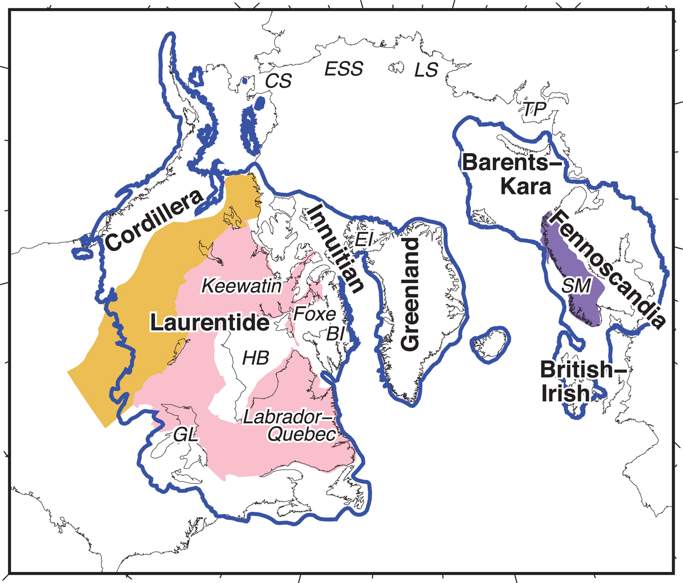
Fig. 1. Location of Northern Hemisphere ice sheets at the LGM (21 kyr BP): Cordillera, Laurentide, Innuitian, Greenland, Barents-Kara, Fennoscandia and British-Irish Ice Sheets (blue line; Dyke, Reference Dyke2004; Hughes and others, Reference Hughes, Gyllencreutz, Lohne, Mangerud and Svendsen2016; Gowan and others, Reference Gowan, Tregoning, Purcell, Montillet and McClusky2016). The locations of the three domes of Laurentide Ice Sheet: Labrador-Quebec, Keewatin and Foxe. The areas mentioned in this study include the Hudson Bay (HB), the Great Lakes (GL), Baffin Island (BI), Ellesmere Island (EI), Taimyr Peninsula (TP), Laptev Sea (LS), East Siberian Sea (ESS) and Chukchi Sea (CS). The yellow area is the Interior Plains, the pink area is the Canadian Shield and the purple area is the Scandinavia Mountains (SM).
Numerical ice-sheet models are widely used to assess the evolution of ice sheets. Ideally, the ice-sheet models are embedded within global circulation models to capture the feedbacks between the climate and the ice sheet. However, this approach is not yet computationally feasible over glacial-interglacial timescales. On the other hand, neither climate reconstructions nor off-line paleo climate simulations provide the temporally and spatially varying boundary conditions required for simulations with stand-alone ice-sheet models. Climate reconstructions are too sparse to provide a spatially detailed temperature distribution and usually do not provide reliable, quantitative precipitation information. Climate simulations rely on reconstructed ice-sheet geometries as a boundary condition and are usually only available as time slice experiments for specific, well constrained periods, such as the LGM or the preindustrial (PI).
The glacial index method synthesizes the necessary boundary conditions by combining the temporal evolution of the climate as deduced from climate reconstructions (often based on an ice core record, since the isotope record is correlated with temperature) with the spatial signature of glacial and interglacial climate modes deduced from a limited number of time slice simulations (e.g., Greve and others, Reference Greve, Wyrwoll and Eisenhauer1999; Marshall and others, Reference Marshall, Tarasov, Clarke and Peltier2000, Reference Marshall, James and Clarke2002; Charbit and others, Reference Charbit, Ritz and Ramstein2002; Rodgers and others, Reference Rodgers2004; Tarasov and Peltier, Reference Tarasov and Peltier2004; Zweck and Huybrechts, Reference Zweck and Huybrechts2005; Charbit and others, Reference Charbit, Ritz, Philippon, Peyaud and Kageyama2007). The basis of this approach is the assumption that to first order climate can be separated into a spatial mode and a temporal index globally modulating it over time. There are several aspects that need to be carefully considered when applying this method. The climate used for forcing the ice-sheet model is generated with a prescribed ice-sheet reconstruction configuration, which causes a circularity between the climate forcing and the resulting ice-sheet simulation. Also, the proxy-based index may not represent the climate on a global scale, and interactions between ice sheet and other climate components cannot be investigated by using this method. However, this approach allows us to investigate the influence of climate forcing and to test ice-sheet model parameters for consistency.
Atmospheric effects (e.g. surface air temperature, solar radiation, precipitation) are important for the evolution of predominantly land-based Northern Hemisphere ice sheets (Oerlemans, Reference Oerlemans1991). Using output from General Circulation Model (GCM) intercomparison projects, the sensitivity of ice sheets to the forcing has been investigated in earlier studies (Pollard, Reference Pollard2000; Charbit and others, Reference Charbit, Ritz, Philippon, Peyaud and Kageyama2007; Fyke and others, Reference Fyke, Eby, Mackintosh and Weaver2014; Yan and others, Reference Yan, Wang, Johannessen and Zhang2014; Dolan and others, Reference Dolan2015). Pollard (Reference Pollard2000) found considerable scatter of surface mass budgets for the Northern Hemisphere ice sheets among the atmosphere-only models from the first generation of The Paleoclimate Modelling Intercomparison Project (PMIP). Same case is also shown in the simulated ice sheets (Charbit and others, Reference Charbit, Ritz, Philippon, Peyaud and Kageyama2007). The simulated Greenland ice sheet during a warm climate has also been found to be highly dependent on the climate forcing (Fyke and others, Reference Fyke, Eby, Mackintosh and Weaver2014; Yan and others, Reference Yan, Wang, Johannessen and Zhang2014; Dolan and others, Reference Dolan2015).
In our study, we used the PMIP3 output to test the sensitivity of atmospheric effects on ice-sheet evolution during the last glacial cycle. PMIP3 is the third phase of the paleoevalution project PMIP to compare different atmosphere-ocean coupled GCMs (Braconnot and others, Reference Braconnot2012). We first simulated Northern Hemisphere ice-sheet evolution with the results of one GCM, COSMOS, by using the glacial index method. We tuned the precipitation to match the past sea-level record at the LGM and treat it as our reference simulation. We then investigated the uncertainties linked to the atmospheric forcing using different models. The ice-sheet configurations used for the PMIP3 model simulations, as well as the other boundary conditions are consistent among all the simulations.
For this paper, our aim is not to gain insight on the evolution of the ice sheets or to ultimately evaluate the skill of any climate models. Instead, we want to test whether the reconstructed ice-sheet evolution is generally consistent with a linear combination of a glacial and interglacial climate state. By comparing with independent ice-sheet reconstructions, we deduce highly sensitive regions and time periods that cannot be simulated with the glacial index method. These cases may indicate the existence of non-linear feedbacks, unresolved processes and incorrect boundary conditions. Secondly, we quantify the uncertainty which arises from uncertain climate forcing, by applying the same method together with output from other PMIP3 models. For GCMs, although forced with the same boundary conditons, the simulated climate is model dependent, and therefore the modelled ice-sheet evolution may also be different.
2. MODEL SET-UP AND EXPERIMENT DESIGN
2.1. The ice-sheet model
The Parallel Ice-Sheet Model (PISM, version 0.7.3) is an open source, three-dimensional thermo-mechanically coupled shallow ice-sheet model (Bueler and Brown, Reference Bueler and Brown2009; Winkelmann and others, Reference Winkelmann2011; Aschwanden and others, Reference Aschwanden, Bueler, Khroulev and Blatter2012; The PISM authors, 2016). We implemented an atmospheric module into the model with a glacial index forcing scheme, based on PISM's extensible atmosphere and ocean coupling feature. The solid earth deformation (GIA) is calculated with the Lingle and Clark method (Lingle and Clark, Reference Lingle and Clark1985; Bueler and others, Reference Bueler, Lingle and Brown2007).
The spatial domain is defined on a Northern Hemisphere polar stereographic grid with 20 km horizontal resolution. On the vertical coordinate, there are 201 unevenly spaced levels above the bedrock and 21 levels downward into the bedrock. The model run starts at 122.9 kyr BP during the Last Interglacial (from 122.9 to 0 kyr BP, Sect. 2.2). The initial conditions are set to the present day. The basal topography data we use are ETOPO1 (Amante and Eakins, Reference Amante and Eakins2009). The basal geothermal heat flux data are from Davies (Reference Davies2013). All of the data are bilinearly interpolated onto the 20 km model grid. The relative sea-level time series for the land-sea mask is from Rohling and others (Reference Rohling2014, Fig. 2b).

Fig. 2. (a) The NGRIP ice core δ18O record (Andersen and others, Reference Andersen2004) and the corresponding value of the glacial index. (b) The reconstructed relative sea-level change from Rohling and others (Reference Rohling2014, dark blue line) with $1 \; \sigma$ error bars (light blue), Lambeck and others (Reference Lambeck, Rouby, Purcell, Sun and Sambridge2014, black line) and the modelled sea-level equivalent (SLE) of the Northern Hemisphere ice sheets (red) using COSMOS-AWI. The correlation coefficient between SLE (PISM) and RSL (Rohling 2014) is 0.865. (c) Separated sea level equivalent (SLE) of Greenland ice sheet (green), Eurasian ice sheets (black), North American ice sheets (blue) and Northern Hemisphere ice sheets (red) through the last glacial cycle.
The stress balance computation used for ice dynamics is a combination of the shallow ice approximation (SIA) and shallow shelf approximation (SSA). The Glen-Paterson-Budd-Lliboutry-Duval flow law (Paterson and Budd, Reference Paterson and Budd1982; Lliboutry and Duval, Reference Lliboutry and Duval1985; Aschwanden and others, Reference Aschwanden, Bueler, Khroulev and Blatter2012) is used to relate stress and strain rates. Surface mass balance is computed by the semi-empirical positive degree-day (PDD) scheme (Reeh, Reference Reeh1989). Instead of taking radiative heat fluxes directly as forcing, it assumes that the melt rate of snow and ice is proportional to the sum of the positive surface air temperature values over the year. The related PDD parameters (Table S1) are the amount of snow or ice that melts per Kelvin and day. They are calibrated using measurements from the present day ice sheets and glacier surfaces (Ritz, Reference Ritz1997). The PDD method is widely used for paleo ice-sheet modelling since it requires less variables than energy balance models and is computationally efficient (e.g., Greve and others, Reference Greve, Wyrwoll and Eisenhauer1999; Marshall and others, Reference Marshall, Tarasov, Clarke and Peltier2000, Reference Marshall, James and Clarke2002; Charbit and others, Reference Charbit, Ritz and Ramstein2002; Rodgers and others, Reference Rodgers2004; Tarasov and Peltier, Reference Tarasov and Peltier2004; Zweck and Huybrechts, Reference Zweck and Huybrechts2005; Charbit and others, Reference Charbit, Ritz, Philippon, Peyaud and Kageyama2007). The model parameters used in our simulations are summarized in Table S1. Further details of the PDD scheme, the ice dynamics, the subglacial dynamics and the ice shelf dynamics are provided in the supplementary materials.
2.2 The climate forcing
The simulation is driven by a glacial index I(t) combined with monthly near-surface air temperature (T mon) and precipitation (P mon) fields at two-time slices, the LGM (21 kyr BP) and present day (PD). The glacial index is derived from the North Greenland Ice Core Project (NGRIP) δ18O 50-year average record (Andersen and others, Reference Andersen2004, 122.95 kyr BP–0 kyr BP, Fig. 2a). The value of I is 1 for LGM (I LGM = 1, t = 21 kyrBP) and 0 for PD (I PD = 0, t = 0 kyrBP), which represent full glacial conditions and interglacial conditions respectively. The index is linearly interpolated for the other time periods using the following formula:

Present day 2-m air temperature fields are from NCEP/NCAR Reanalysis long-term monthly mean datasets (Kalnay and others, Reference Kalnay1996, 1981–2010, Fig. S1c-d). Precipitation fields are from GPCP long-term monthly mean datasets (Adler and others, Reference Adler2003, 1981–2010, Fig. S2c-d). For the LGM, the temperature and precipitation is from the Earth System Model COSMOS (ECHAM5-JSBACH-MPIOM) with T31 resolution at Alfred Wegener Institute Helmholtz Center for Polar and Marine Research (Zhang and others, Reference Zhang, Lohmann, Knorr and Xu2013, COSMOS-AWI). This dataset represents a steady climate state at the LGM (Fig. S1a-b and S2a-b). The COSMOS Earth system model has been used and tested against different paleo climate scenarios and is appropriate as the climate forcing for our PISM simulation. External forcing and boundary conditions are set according to the PMIP3 protocol (see details in Section 2.3). The data are bilinearly interpolated onto the model grids.
The paleoclimate fields calculated using the index method are based on the linear relationship between PD and LGM:


The glacial index approach is similar as in previous studies (Greve and others, Reference Greve, Wyrwoll and Eisenhauer1999; Marshall and others, Reference Marshall, Tarasov, Clarke and Peltier2000; Charbit and others, Reference Charbit, Ritz, Philippon, Peyaud and Kageyama2007). As is shown in Fig. 2a, for much of the Holocene, the late Eemian or much of the LGM, I(t) can be <0 or >1, which results in warmer conditions than PD or colder conditions than 21 kyr BP. Equation (4) is used to avoid negative precipitation. Equation (5) is a precipitation correction due to surface elevation (H) change, based on the exponential relationship between water vapour saturation pressure and temperature in the upper atmosphere. A tuning parameter (β = 0.75 km−1) is used for reducing the precipitation at high elevations, so that the modelled ice-sheet volume matches the global sea-level curve at the LGM within those observation uncertainties (Whitehouse and others, Reference Whitehouse, Bentley and Le Brocq2012; Austermann and others, Reference Austermann, Mitrovica, Latychev and Milne2013; Lambeck and others, Reference Lambeck, Rouby, Purcell, Sun and Sambridge2014). By increasing β, the amount of precipitation can be reduced considerably. Otherwise, the modelled sea-level equivalent at the LGM can be twice as large as the far field sea-level record. A slight modification is made for the present day precipitation to eliminate the error caused by the precipitation elevation correction:

A freely evolving lapse rate correction for temperature is not included since the climate forcing at the LGM has already accounted for temperature change due to elevation change. The other reason is that we want to test the sensitivity of ice sheet to surface temperature from different GCMs. Including a temperature lapse rate correction will give the ice-sheet elevation one extra degree of freedom to evolve.
2.3. PMIP3 model comparison experiment
In this experiment, we focus on the influence of variance in GCM on the simulation of ice sheets. Climates modelled by different GCMs vary between each other and contain model deficiencies. Using the same parameters from the initial experiment from COSMOS-AWI, we run the same simulation using the other PMIP3 ensemble members (Meinshausen and others, Reference Meinshausen2011; Braconnot and others, Reference Braconnot2012). For present day conditions, we first use the reanalysis products (as described in Section 2.2) to make sure all the experiments have consistent PD conditions. We name this set of experiments ‘PMIP3-PDobs’. Further discussion regarding the choice of reanalysis products or GCM preindustrial (PI) output is given in Sect. 4.2.
In total there are nine PMIP3 models available online (Table 1). For model comparison, all models use the same boundary conditions (orbital parameters, trace gases and ice-sheet configuration). The ice-sheet configuration at the LGM used in the PMIP3 experiment is a blended product obtained by averaging three different ice-sheet reconstructions: ICE-6G, GLAC and ANU (Abe-Ouchi and others, Reference Abe-Ouchi2015). More details of the protocols can be found at https://pmip3.lsce.ipsl.fr/. As with the model set-up described before, monthly climatology data for surface air temperature and precipitation from the GCMs are used as input.
Table 1. PMIP3 model descriptions. All the models are prescribed with the same boundary conditions: (1) orbital parameters (Berger, Reference Berger1978): eccentricity = 0.018994, obliquity = 22.949°, perihelion-180° = 114.42°. (2) trace gases (Monnin and others, Reference Monnin2001; Dällenbach and others, Reference Dällenbach2000; Flückiger and others, Reference Flückiger1999): CO2 = 185 ppm, CH4 = 350 ppb, N2O = 200 ppb. (3) the ice-sheet configuration at LGM is a blended product by averaging three different ice-sheets reconstructions (Abe-Ouchi and others, Reference Abe-Ouchi2015)
*AWI: Alfred Wegener Institute Helmholtz Center for Polar and Marine Research. NCAR: National Center for Atmospheric Research. CNRM/CERFACS: Centre National de Recherches Météorologiques / Centre Européen de Recherche et Formation Avancée, Calcul Scientifique. FUB: Freie Universitaet Berlin, Institute for Meteorology. LASG/IAP: LASG, Institute of Atmospheric Physics, Chinese Academy of Sciences and CESS,Tsinghua University. GISS: NASA Goddard Institute for Space Studies. IPSL: Institut Pierre-Simon Laplace. MIROC: Japan Agency for Marine-Earth Science and Technology, Atmosphere and Ocean Research Institute (The University of Tokyo), and National Institute for Environmental Studies. MPI: Max-Planck-Institut für Meteorologie (Max Planck Institute for Meteorology). MRI: Meteorological Research Institute.
3. RESULTS
3.1. Ice-sheet evolution through the last glacial cycle
In this section, we analyze the simulated ice-sheet evolution with forcing from COSMOS-AWI both spatially and temporally. We compared the performance of the simulated ice sheets with reconstructions of sea level and ice-sheet extent.
3.1.1. The temporal evolution of ice-sheet volume
Figure 2b shows a comparison between simulated ice volume (in units of eustatic Sea Level Equivalent, SLE, red line) and relative sea-level reconstructions (Rohling and others, Reference Rohling2014; Lambeck and others, Reference Lambeck, Rouby, Purcell, Sun and Sambridge2014). Generally, the modelled ice volume change resembles a sawtooth curve with slow ice-sheet buildup and fast retreat. The total ice volume decreases slightly in response to higher temperature before 121 kyr BP. After that, the ice volume increases with several fluctuations, for instance, at 109 kyr BP, 91 kyr BP and 86 kyr BP. In response to the cold signals in NGRIP during Marine Isotope Stage 4 (MIS 4, 80–60 kyr BP), the ice volume increases significantly by up to 90 m SLE. These features agree well with the reconstructed curve, but there are some differences. During MIS 4, the modelled local sea-level minimum happens ~7 kyr later than the relative sea-level curve. The starting times of the modelled ice-sheet retreat are later than the reconstruction, indicating that the modelled ice-sheet responses are less sensitive. One potential reason could be that a cryo-hydrologic warming to the ice which can cause nonlinear ice flow response is not currently captured by PISM (Colgan and others, Reference Colgan, Sommers, Rajaram, Abdalati and Frahm2015). A mismatch of the age models of the NGRIP data and the Rohling sea-level curve can also cause this inconsistency. The amplitude of the SLE variability is not as large as the reconstructed time series, especially during the glacial inception. This is probably because we use constant PDD parameters for calculating the surface ablation, which might cause a partial mismatch between the simulated results and the reconstructed sea level due to different insolation contributions.
Between 60 kyr BP and 25 kyr BP, the simulated SLE fluctuated with higher frequency in response to the high amplitude millennial-scale variability in the ice core, which are called Dansgaard-Oeschger (DO) events. The regions that mainly contributed to the ice-sheet variations were around the ice-sheet margins (not shown). The total ice-sheet volume reached its maximum (~120 m SLE) at ~24 kyr BP, and remained near this value until 15 kyr BP. If a sea-level contribution of 10 m from Antarctica Ice Sheets is included (Whitehouse and others, Reference Whitehouse, Bentley and Le Brocq2012), the maximum SLE value is comparable with the far-field sea-level records (134 m; Austermann and others, Reference Austermann, Mitrovica, Latychev and Milne2013; Lambeck and others, Reference Lambeck, Rouby, Purcell, Sun and Sambridge2014). Afterwards, it retreated rapidly to half of its maximum value by 13.5 kyr BP. A slight increase in ice volume happened at 11.7 kyr BP, corresponding with the Younger Dryas. The total ice volume continued decreasing until 9 kyr BP, then became stable with 6-7 m SLE remaining. The final timing of deglaciation is earlier than the geological constraints (Lambeck and others, Reference Lambeck, Rouby, Purcell, Sun and Sambridge2014; Cuzzone and others, Reference Cuzzone2016; Ullman and others, Reference Ullman2016). There are large uncertainties in the reconstructed sea level during the Holocene (Rohling and others, Reference Rohling2014), while the variability of the simulated ice volume is insignificant.
The individual sea-level contributions in Greenland, Eurasian and North American (excluding Greenland) ice sheets varied between different marine isotope stages (Fig. 2c). The Greenland ice sheet (green) was the main contributor to sea-level fall during MIS 5e, and after that remained relatively stable with 10 m SLE until the deglaciation (~14 kyr BP). North American ice sheets (blue) started to build up from MIS 5d, while the Eurasian ice sheets (black) development was restricted before MIS 4. The amplitude of ice-sheet volume change response to DO events for Eurasian ice sheets was smaller than North American ice sheets. The maximum ice volume of Eurasian ice sheets was during MIS 2 with 30 m, and ~80 m for North American ice sheets. At 15 kyr BP, North American ice sheets were slightly larger than at 20 kyr BP, while the Eurasian ice sheets were smaller than before. The SLE increase during the Younger Dryas was more than 6 m, mainly derived from the North American ice sheets in our simulation. However, far-field sea-level evidences show that sea-level rise slowed down during the Younger Dryas (Bard and others, Reference Bard, Hamelin and Delanghe-Sabatier2010), with extensive end moraines found for the Eurasian ice sheets (Cuzzone and others, Reference Cuzzone2016). The timing of final deglaciation for the Eurasian ice sheets shows agreement with previous studies (9.1 kyr BP; Cuzzone and others, Reference Cuzzone2016), while it is too early for the North American ice sheets (~7 kyr BP; Ullman and others, Reference Ullman2016).
3.1.2. Spatial distribution of ice sheets
Snapshots of ice-sheet thickness at different key periods are shown in Fig. 3. Consistent with the SLE change (Fig. 2b), the extent of the Greenland ice sheet shrank slightly during MIS 5e. As the climate became colder, a thin ice sheet started to build up along the northeast coast of North America, in the region of Baffin Island and the Labrador-Quebec sector. It advanced westward into the Interior Plains during MIS 5d, when the Cordilleran Ice Sheet and the Scandinavian Ice Sheet also started to build up as low profile, thin ice sheets. During MIS 5c, the ice sheets retreated again with ice remaining on Baffin Island and Ellesmere Island. Compared to MIS 5d, the MIS 5b ice sheets were much thicker in Baffin Island and the Labrador-Quebec sector. According to Kleman and others (Reference Kleman2010), an ice divide close to the Labrador coast in the Quebec sector existed during MIS 5b or 5d, and may indicate the location of glacial inception for North American ice sheets started around the northeast coast. The Cordilleran Ice Sheet also grew notably during MIS 5b. Ice sheet retreat happened during MIS 5a, with ice remaining on the northeast coast of North America and ice caps in the Barents-Kara area.
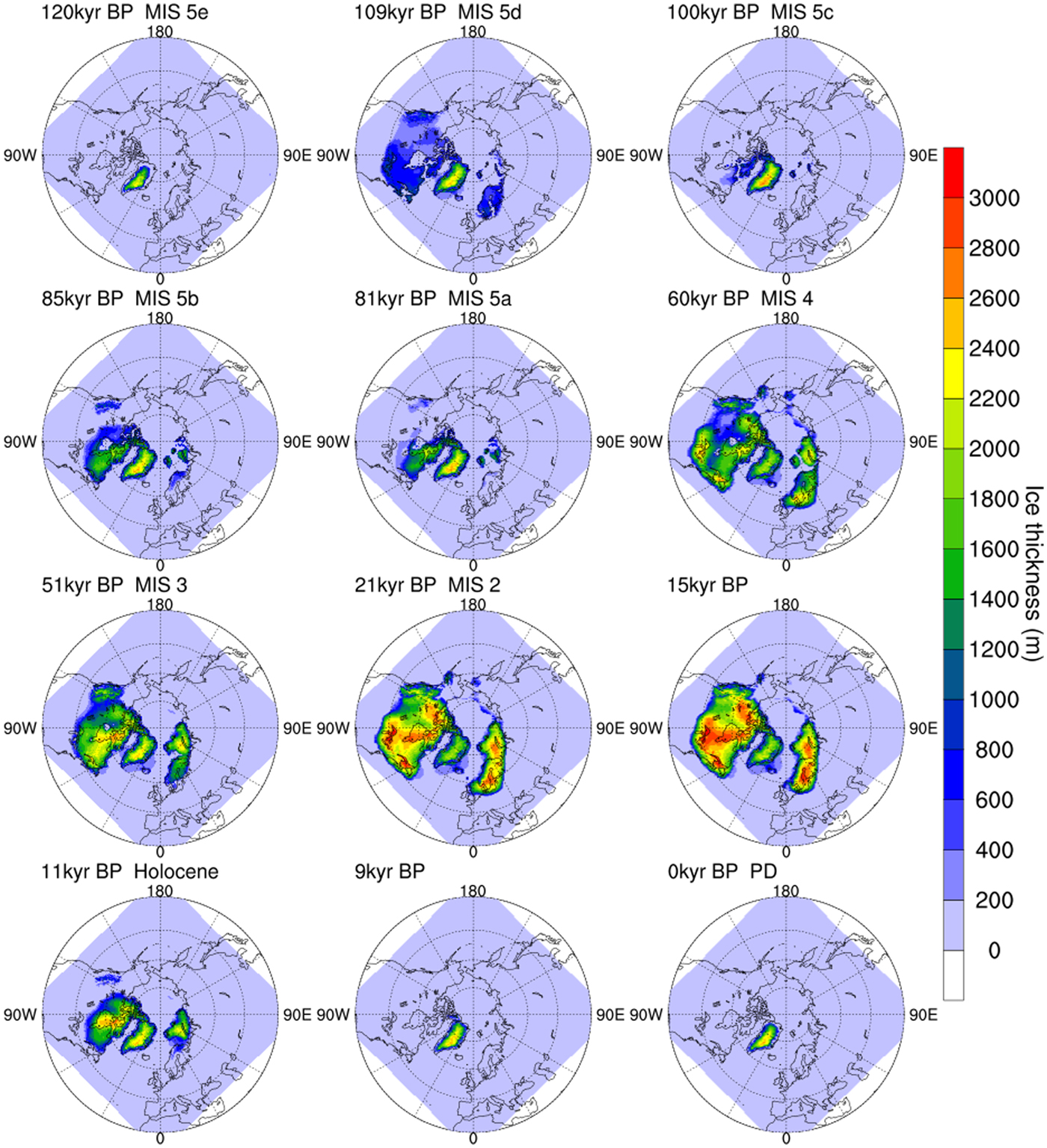
Fig. 3. Modelled ice thickness (m) evolution through the last glacial cycle at different climate stages. The simulation is forced by the climatology monthly mean surface air temperature and precipitation from COSMOS-AWI.
During MIS 4, the ice sheets extended far further south in both North America and Eurasia. For North America, the ice sheets built up in Labrador-Quebec, Keewatin, the Great Lakes and Cordilleran areas separately, leaving the Hudson Bay Lowlands, the western part of Hudson Bay and south of Keewatin almost ice free. Large ice sheets grew at the southern margin of Laurentide ice sheet prior to the LGM (Wood and others, Reference Wood, Forman, Everton, Pierson and Gomez2010; Carlson and others, Reference Carlson, Tarasov and Pico2018), which our simulations are able to reproduce. For Eurasia, the Barents-Kara Ice Sheet, the Scandinavian Ice Sheet and the British-Irish Ice Sheet built up, while the Scandinavian Ice Sheet and Barents-Kara Ice Sheet separated. During MIS 3, the total ice volume increased gradually, accompanied with fluctuations due to the DO events. This is inconsistent with recent studies showing that the Laurentide Ice Sheet advanced rapidly towards the LGM (Dalton and others, Reference Dalton, Finkelstein, Barnett and Forman2016; Carlson and others, Reference Carlson, Tarasov and Pico2018). During this period, the Scandinavian Ice Sheet and Barents-Kara Ice Sheet merged, the western Laurentide Ice Sheet and eastern Laurentide Ice Sheet merged, and the Cordilleran Ice Sheet and the Laurentide Ice Sheet merged. At ~21 kyr BP, the Northern Hemisphere ice sheets reached their maximum extent.
The ice domes in the Keewatin and Labrador sectors were probably dynamically independent for most of the time before the LGM. The Labrador dome expanded southward earlier than the Keewatin sector at around MIS 4. For Eurasian ice sheets, geological evidence indicates that the Barents-Kara Ice Sheet extended further east to the Taimyr Peninsula prior to the LGM, and the Barents-Kara Ice Sheet became smaller while the Scandinavian Ice Sheet became bigger during each successive glaciation (Svendsen and others, Reference Svendsen2004). In other words, the Eurasian ice sheets advanced progressively further southwest from MIS 4 to the LGM. In our simulation, the Barents-Kara Ice Sheet did not build up prior to MIS 4 and there was no change in ice-sheet extent through time. This is likely because the large-scale North American ice sheet build-up changed the atmospheric stationary waves. The modified atmospheric circulation favoured the growth of southwestern Eurasian ice sheets (Roe and Lindzen, Reference Roe and Lindzen2001; Liakka and others, Reference Liakka, Nilsson and Löfverström2012; Löfverström and others, Reference Löfverström, Caballero, Nilsson and Kleman2014). Since the index method cannot account for differences in atmospheric circulation due to different ice-sheet configurations, it is unsurprising that there is this mismatch.
The ice-sheet configuration during the LGM is relatively well known. There were three major domes of Laurentide Ice Sheet: Labrador, Keewatin and Foxe (Prest, Reference Prest1968; Bryson and others, Reference Bryson, Wendland, Ives and Andrews1969; Dyke and Prest, Reference Dyke and Prest1987; Margold and others, Reference Margold, Stokes and Clark2015), which can also be observed in our simulation. The North American ice sheets extended southward to 40°N with ice sheet thickness up to 3000 m. The interior of Alaska was ice free during the LGM. For Eurasia, the ice-sheet covered the Barents-Kara Sea, the Scandinavia and extended southwest to the British-Irish area.
Most of the Northern Hemisphere ice sheets started to retreat at ~15 kyr BP, while the British-Irish Ice sheet retreated earlier at 16.5 kyr BP. By ~13 kyr BP, the total ice volume decreased to half of its maximum volume (Fig. 2b), with ice covered regions persisting on Hudson Bay and the Canadian Shield, the center of Cordilleran region, most of Barents-Kara Sea and part of Scandinavia. By 9 kyr BP, all the ice sheets completely retreated except the Greenland ice sheet, which is slightly too early for the Laurentide Ice Sheet (Dyke, Reference Dyke2004; Lambeck and others, Reference Lambeck, Rouby, Purcell, Sun and Sambridge2014; Cuzzone and others, Reference Cuzzone2016; Ullman and others, Reference Ullman2016).
For the simulated conditions at present day (0 kyr BP), the Greenland ice sheet volume is ~2.4 × 10¹⁵ m3 (5.8 m SLE), with a maximum thickness of 2694 m and an ice covered area of 1.9 × 10¹²m2. The magnitude is comparable with the previous studies (e.g., Mote, Reference Mote2003; Fettweis, Reference Fettweis2007).
3.2. Sensitivity of ice-sheet simulations to atmospheric forcing from the PMIP3 experiments
Figure 4a shows the SLE time series from experiment PMIP3-PDobs. Most models succeeded in reproducing the observed sea-level fall (100 m to 150 m) at the LGM, except CNRM-CM5 and MRI-CGCM3 (16 and 49 m, respectively). The total ice volume in GISS-E2-R is relatively large during cold stages, and smaller during warm stages, compared to the other models. The RMSD relative to the reference simulation for the SLE are calculated in Fig. 5 (black circles). The models that are most different from our reference model are CNRM-CM5 and MRI-CGCM3 (RMSD values are 48 and 36 m, respectively). The other models are more consistent with each other, with a RMSD <12 m.
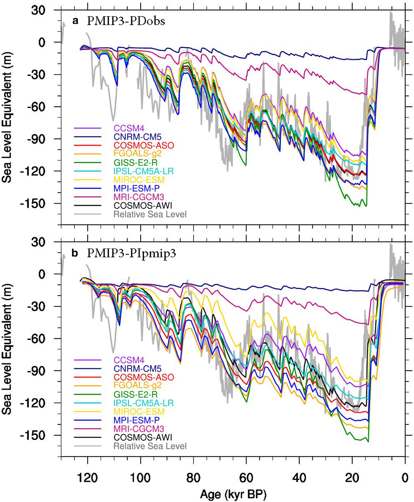
Fig. 4. Modelled sea-level equivalent (SLE) of Northern Hemisphere ice sheets change through the last glacial cycle using the output of PMIP3 models. (a) Experiment PMIP3-PDobs, with climate forcing of present-day conditions from reanalysis products (1981–2010) and the LGM conditions from PMIP3 GCM output. (b) Experiment PMIP3-PIpmip3, with climate forcing of present-day conditions from PMIP3 preindustrial (PI) output and LGM conditions from PMIP3 GCM output.
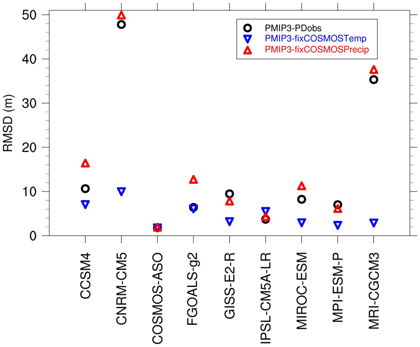
Fig. 5. RMSD of SLE when compared to the reference simulation (COSMOS-AWI) for different PMIP3 models. Black circles are from experiment PMIP3-PDobs, blue triangles are from experiment PMIP3-fixCOSMOSTemp, red triangles are from experiment PMIP3-fixCOSMOSPrecip.
The models exhibit large differences at the LGM, both in ice-sheet thickness and extent (Fig. 6). Consistent with the SLE time series, the ice sheets from CNRM-CM5 are small in extent, with ice sheets in the western coast of North America, Keewatin region, Labrador, southern Greenland and the Scandinavia Mountains. MRI-CGCM3 shows similar results with more ice covering Hudson Bay, Greenland and Barents-Kara Sea. Compared with the results from COSMOS-AWI, there is less ice in North America in GISS-E2-R. Instead, there is ice build up in Siberia, where there is no evidence of an LGM Ice Sheet (Niessen and others, Reference Niessen2013, Fig. 4, green line). For the other models, the general patterns are similar to the COSMOS-AWI model, except for CCSM4 and FGOALS-g2, which have ice-sheet growth on the East Siberian Sea, Laptev Sea and Chukchi Sea.
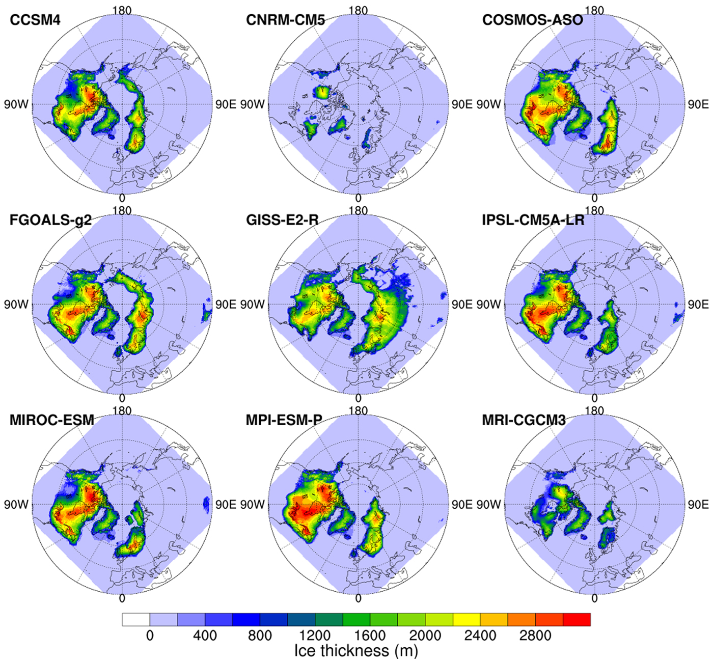
Fig. 6. Modelled ice thickness at the Last Glacial Maximum (LGM, 21 kyr BP) using the PMIP3 model output from experiment PMIP3-PDobs.
In order to investigate why the ice sheets have such a diverse range of extents, when the only difference is the atmospheric forcing, we compared the surface air temperature and precipitation. We found that the ice-sheet extent is strongly related to the summer surface air temperature. Figure S3 shows the Probability Distribution Functions of the surface air temperature and precipitation over ice-sheet margins and Northern Hemisphere during different seasons. The ice-sheet margins are generally located where summer temperatures are confined to between − 5 and 5°C. The spatial distribution also shows a similar pattern (Fig. 7). The ice-sheet extent pattern during the LGM resembles the summer surface air temperature pattern, where the ice-sheet margin is similar to the − 5°C isothermal lines. For precipitation, no clear relationship emerges.
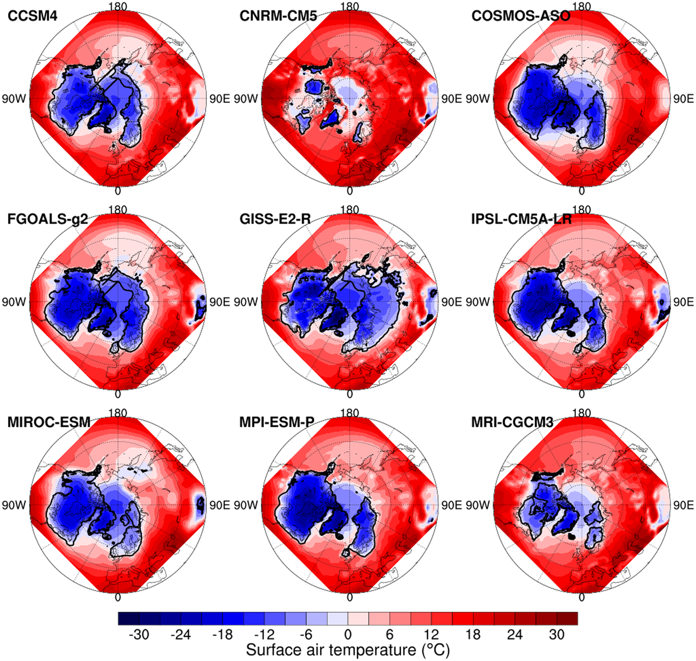
Fig. 7. The surface air temperature at the Last Glacial Maximum (LGM) in summer (JJA) for different models that participated in PMIP3 and the ice-sheet margins at the LGM (black lines).
To study the individual roles of temperature and precipitation, we conducted two additional sets of experiments. One experiment keeps the temperature the same as COSMOS-AWI, while using the precipitation from the PMIP3 models (PMIP3-fixCOSMOSTemp). The other experiment is the opposite (PMIP3-fixCOSMOSPrecip). When forced with the same temperature, the simulated SLE evolution has closer agreement between the simulations (Fig. 8a) with RMSD values <11 m (Fig. 5, blue triangles). The ice-sheet extent at the LGM also shows more consistency between simulations (Fig. S4), but with quite different ice-sheet thickness distribution, which is mainly caused by the differences in precipitation. The results from PMIP3-fixCOSMOSPrecip are more similar to the experiments from PMIP3-PDobs (Fig. 8b, S5). The failure of ice sheet build up at the LGM, especially for CNRM-CM5 and MRI-CGCM3, are mainly a result of a warm temperature bias. This contributes to a larger variability compared with the PMIP3-PDobs simulations, with larger RMSD values in 6 out of 9 models (Fig. 5, red triangles).
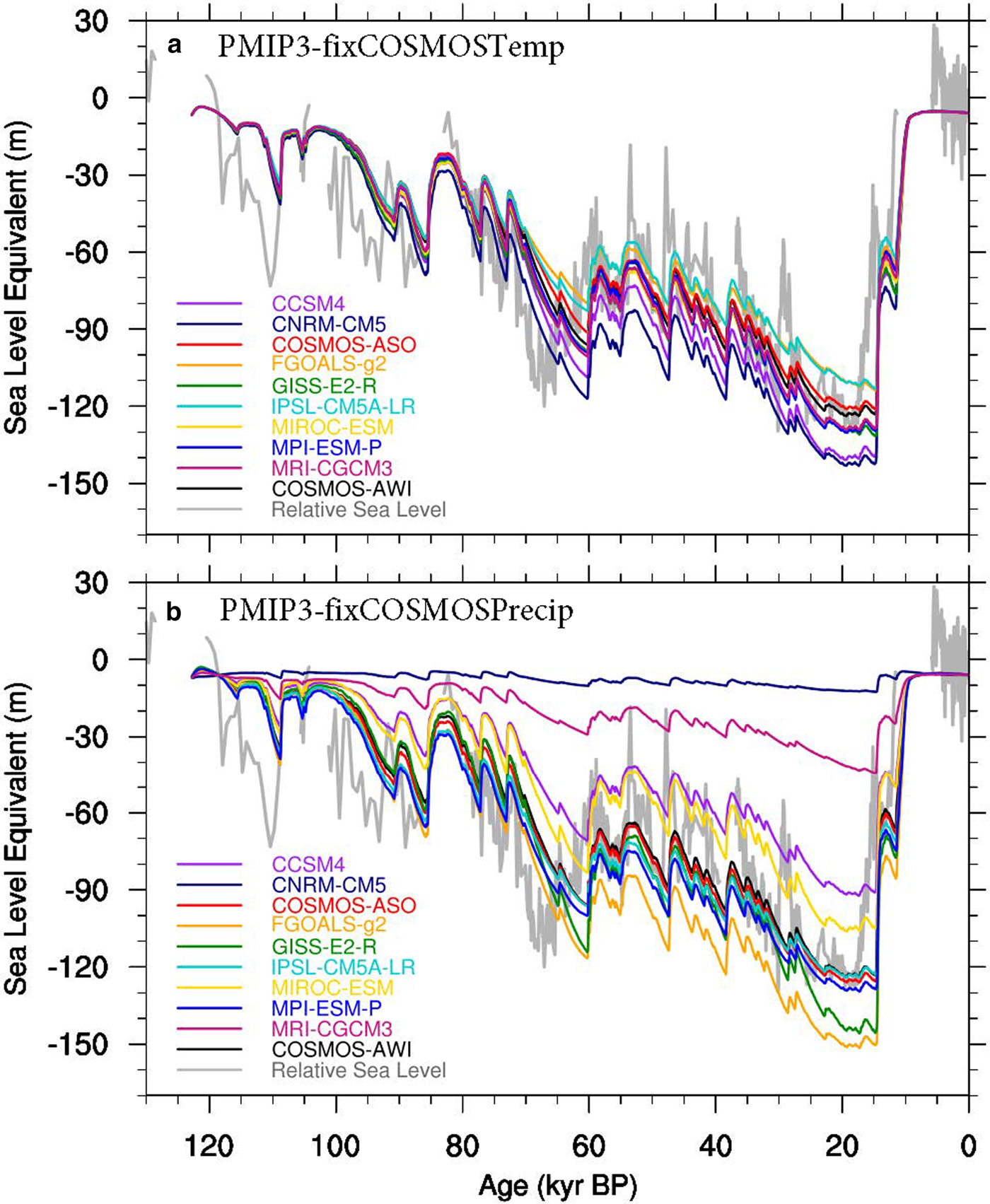
Fig. 8. Modelled sea-level equivalent (SLE) of Northern Hemisphere ice sheets change through the last glacial cycle using the PMIP3 model output. (a) PMIP3-fixCOSMOSTemp, with surface air temperature from COSMOS-AWI, precipitation from PMIP3 models. (b) PMIP3-fixCOSMOSPrecip, with precipitation from COSMOS-AWI, surface air temperature from PMIP3 models.
4. DISCUSSIONS
4.1. The glacial index method
In the previous section, we compared the simulated ice sheets to geological evidence. Consistent with previous studies that used the glacial index method (e.g. Marshall and others, Reference Marshall, James and Clarke2002; Tarasov and Peltier, Reference Tarasov and Peltier2004; Charbit and others, Reference Charbit, Ritz, Philippon, Peyaud and Kageyama2007), we confirm that the method is capable of capturing the first order pattern of the North Hemisphere ice sheet evolution. Furthermore, more features (for example, the glacial inception pattern and the ice-sheet configuration at the LGM) are captured with forcing from COSMOS-AWI than in previous studies (e.g. Marshall and others, Reference Marshall, James and Clarke2002; Charbit and others, Reference Charbit, Ritz, Philippon, Peyaud and Kageyama2007).
However, several aspects need to be considered carefully when using this method. First of all, there is a circularity between the ice-sheet simulation and the GCM simulation. The GCM output used as climate forcing is based on a reconstructed ice-sheet configuration with fixed ice-sheet topography and surface albedo (Abe-Ouchi and others, Reference Abe-Ouchi2015). Due to higher elevation and higher albedo over the ice surface, the surface temperature at the LGM is much lower over the prescribed ice-sheet regions than that of bare-land regions (Fig. S1). The strong temperature gradient at the ice-sheet margins restricted the southern extent of the simulated ice sheets. More precipitation is simulated in the southern margins of the ice sheets at the LGM than PD (Fig. S2). This precipitation bias resulted in more ice buildup around the southern margins of the ice sheets.
The feedbacks between the ice sheet, atmosphere and ocean cannot be inferred with this method. Recent studies found that large ice sheets can significantly modify the stationary waves or jet streams, and the atmospheric response can reorganize the structure of the ice sheets (Liakka and others, Reference Liakka, Nilsson and Löfverström2012; Ullman and others, Reference Ullman, LeGrande, Carlson, Anslow and Licciardi2014; Löfverström and others, Reference Löfverström, Caballero, Nilsson and Kleman2014, Reference Löfverström, Liakka and Kleman2015). Also, the final deglaciation of the modelled ice sheets is too early compared to the geological evidence, especially in North America (Dyke, Reference Dyke2004; Rohling and others, Reference Rohling2014; Cuzzone and others, Reference Cuzzone2016; Hughes and others, Reference Hughes, Gyllencreutz, Lohne, Mangerud and Svendsen2016; Ullman and others, Reference Ullman2016). This indicates that these regions might still be cold during that time, while the linear interpolation based on the Greenland ice core record may not have the signal. The fluctuations in the Greenland record may reflect local climate changes that are on orbital and millennial timescales, which may not be global in nature (Seguinot and others, Reference Seguinot, Rogozhina, Stroeven, Margold and Kleman2016; Banderas and others, Reference Banderas, Alvarez-Solas, Robinson and Montoya2018). Temperature and isotope signals imprinted in Greenland due to regional and global climate conditions change may also be different (Buizert and others, Reference Buizert2014; Pausata and Löfverström, Reference Pausata and Löfverström2015).
To adequately capture the feedbacks between ice sheets and the atmosphere, it is necessary to use GCMs bidirectionally coupled to ice-sheet models. An approach of coupling ice sheet models to Earth system Models of Intermediate Complexity (EMICs, Claussen and others, Reference Claussen2002) has been used (e.g., Charbit and others, Reference Charbit, Kageyama, Roche, Ritz and Ramstein2005; Ganopolski and others, Reference Ganopolski, Calov and Claussen2010; Fyke and others, Reference Fyke2011; Bauer and Ganopolski, Reference Bauer and Ganopolski2017). However, the spatial grids from EMICs are very coarse. Despite the computational expensive for long-duration simulations, coupling to a sophisticated General Circulation Model (GCM) could be an effective way for solving orbital timescale problems with higher resolution and more sophisticated atmospheric dynmaics (Ziemen and others, Reference Ziemen, Kapsch, Klockmann and Mikolajewicz2019). Combined with Regional Climate Models (RCMs), GCM simulations can be enhanced to solve regional conditions over the ice-sheet margins (Pollard, Reference Pollard2010). In this case, atmospheric forcing that is taken from GCMs needs to be better constrained.
4.2. The atmospheric forcing from GCMs
As is shown in Section 3.2, the summer surface air temperature seems to be an important control on ice-sheet extent. This is consistent with previous studies showing that summer ablation is more important than snow accumulation in the winter for the evolution of the ice sheets (e.g. Gallée and others, Reference Gallée1992). The differences in ablation among GCMs can considerably influence the resultant surface mass balance. The large variability in GCM directly translates into a large variability in simulated ice sheets. We speculate that the differences in simulated surface air temperature are the consequence of the different albedo schemes employed by the GCMs. By calculating the ratio of upwelling shortwave radiation and downwelling shortwave radiation at the surface, we obtain significant differences between the models (Fig. S6).
In winter and colder areas, accumulation is a more prominent process than ablation. From our simulations, a multi-domed pattern at the LGM can be observed in almost all of the model results (Fig. 6). According to the present day precipitation pattern (Fig. S2c-d), precipitation is large along the coast of North America and Europe, while the middle of the continents is relatively dry, especially in the Keewatin region. So how did ice-sheet domes form in these regions? Investigating the temperature and precipitation patterns, we find that in all the models, there was more precipitation in winter in Keewatin at the LGM than present day (Fig. 9), which resulted in accumulation in that region. Also, as is shown in experiment PMIP3-fixCOSMOSTemp, the difference of precipitation pattern could strongly result in a change of the ice-sheet geometry.

Fig. 9. The Precipitation (Precip) difference between Last Glacial Maximum (LGM) and Present Day (PD) in winter (DJF) for different models that participated in PMIP3 (LGM minus PD).
In our PMIP3 experiments, we prescribed the present day climate by using the reanalysis products from 1981 to 2010. The simulated ice sheets varied significantly even though we only changed the LGM climate. In order to make the model comparison more consistent, we replaced the reanalysis products with the modelled PMIP3 preindustrial GCM output and ran the experiments again (PMIP3-PIpmip3).
Comparing the sea-level equivalent time series (Fig. 4b) with the one from PMIP3-PDobs (Fig. 4a), we find that the curves show a similar pattern, but are more scattered. The differences in sea-level equivalent for Greenland at present day can be up to 6 or 7 meters due to the different Preindustrial conditions in different models. The simulated ice thickness pattern at the LGM in PMIP3-PIpmip3 is almost the same as in PMIP3-PDobs (Fig. S7). The most distinct result is the one that used MIROC-ESM forcing, with a difference of more than 600 m in the central area of Laurentide Ice Sheet (Fig. S8). Comparing the summer (JJA) surface air temperature difference between the reanalysis products and the PMIP3 PI GCM output, we find that the MIROC-ESM PI temperatures exhibit a large warm bias over the northern hemisphere continents (Fig. S9). This resulted in less ice-sheet buildup than in the PMIP3-PDobs experiment. For the other models, the ice thickness difference is <600 m, with slightly thicker ice in Eurasia and most of northern North America except for Hudson Bay and Arctic Archipelago in the PMIP3-PIpmip3 experiments (Fig. S8). Comparing the corresponding summer temperature differences (Fig. S9), we find that the anomaly patterns also matched, with a warmer climate leading to a smaller ice volume and a colder climate resulting in a larger ice volume. For most of the PMIP3 models (COSMOS-ASO, FGOALS-g2, GISS-E2-R, IPSL-CM5A-LR, MPI-ESM-P, MRI-CGCM3), the GCM preindustrial conditions are generally colder than the reanalysis products, resulting in a larger ice sheets. This is probably because the reanalysis products are from a time period of 1981–2010, which contains the hottest years of the past century and the climate is perturbed by increased greenhouse gases.
4.3. PDD and surface energy balance
The semi-empirical PDD method is applied for computing the surface ablation. It uses only the surface temperature for computing melt. The PDD scaling parameters are obtained with measurements from modern glacier conditions, while different glaciers or paleo scenarios might give different values. It may underestimate the influence of shortwave radiation for the surface melt, which has been considered as a major driver for glacial cycles (Van de Berg and others, Reference Van de Berg, Van Den Broeke, Ettema, Van Meijgaard and Kaspar2011; Robinson and Goelzer, Reference Robinson and Goelzer2014; Ullman and others, Reference Ullman, Carlson, Anslow, LeGrande and Licciardi2015; Bauer and Ganopolski, Reference Bauer and Ganopolski2017). In order to assess the validity of the PDD method in our stand-alone simulations, we compared the surface melt simulated by PISM's PDD model to the melt computed by energy-balance model of COSMOS, which uses a much more sophisticated energy-balance scheme but at lower resolution (T31) and with fixed ice-sheet configuration (Fig. 10). For consistency, we also compared the results from PMIP3-PIpmip3, with COSMOS preindustrial and LGM output as climate forcing. The results show good agreements between PDD-based approach and energy-balance based approach. At the LGM, all the results show similar melt pattern around the margins of the North American and Eurasian ice sheets. For the present day and the Eemian, the snow melt extent in the North American and Asian continents in COSMOS is broader. For the Greenland ice sheet, the surface melt patterns still match well, especially in the southernmost region. The simulation with reanalysis products show more melt around Greenland, which is probably because the observational data contain the warming signal of the previous century. Previous studies argued that the Laurentide Ice Sheet would never deglaciate if the PDD approach is used (Ullman and others, Reference Ullman, Carlson, Anslow, LeGrande and Licciardi2015; Bauer and Ganopolski, Reference Bauer and Ganopolski2017). This is why we tuned the precipitation to balance the extra total mass gain (Sect. 2.2). In our simulation, the deglaciation is driven by the index method going towards the Present day state. For the current study, the PDD-based scheme may still be a suitable alternative to computationally expensive surface energy-balance models.
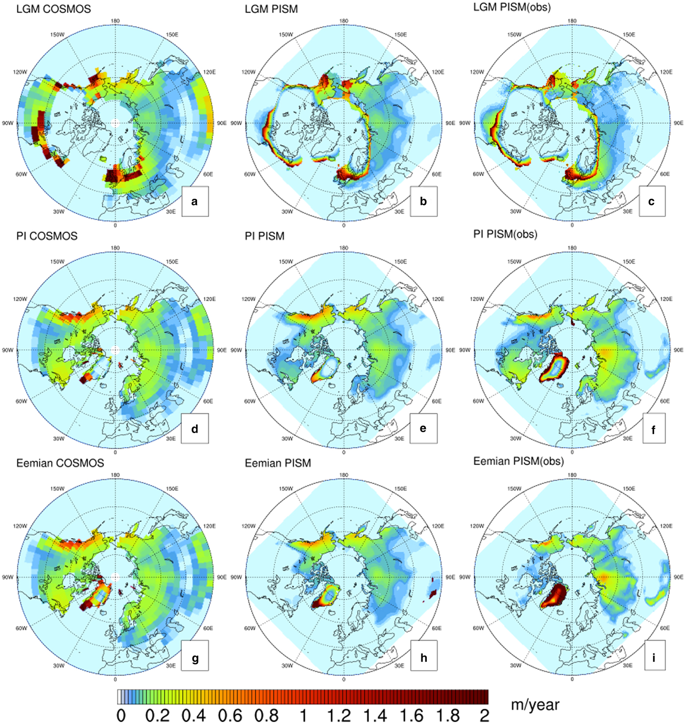
Fig. 10. Comparison of surface melt between energy balance-based scheme from COSMOS (a, d, g) and PDD-based scheme from PISM (b, e, h or c, f, i) at the LGM, present day (PD) and Eemian (Units: m/year). The right panel plots are from the reference simulation (COSMOS-AWI) with reanalysis products at PD and COSMOS GCM at the LGM as climate forcing. The middle panel plots are with COSMOS GCM at preindustrial and the LGM.
4.4. Potential for further investigation
A future step in investigating ice-sheet sensitivity to climate forcing would be the incorporation of more elaborated schemes than PDD (e.g. Krebs-Kanzow and others, Reference Krebs-Kanzow, Gierz and Lohmann2018) where the surface energy balance is taken more explicitly into account. Recent work has also highlighted the role of ocean forcing in driving glacial ice-sheet variability (Bassis and others, Reference Bassis, Petersen and Mac Cathles2017). In our study, we fixed the ocean forcing and did not sample this potential source of climate-driven ice-sheet change. Variability of the ice/substrate interface could also be included in future work (Gowan and others, Reference Gowan, Niu, Knorr and Lohmann2019).
5. CONCLUSIONS
We simulated the Northern Hemisphere ice sheets through the last glacial cycle using the glacial index method based on the NGRIP ice core. Consistent with previous studies, we show that this method is capable of capturing the main features of the Northern Hemisphere ice-sheet evolution during the last glacial cycle. During glacial inception, the ice sheets first built up along the coast of the Quebec-Labrador sector. The growth of the eastern Laurentide Ice Sheet was earlier than the western Laurentide Ice Sheet during the build-up stage (Kleman and others, Reference Kleman2010). For the LGM, the simulated ice extent resembles the geological reconstruction quite well, with the ice-sheet extent extending southward to 40°N, and maximum ice thicknesses up to 3000 m, an ice free Alaska region and a British-Irish Ice sheet (Dyke, Reference Dyke2004; Hughes and others, Reference Hughes, Gyllencreutz, Lohne, Mangerud and Svendsen2016). The Northern Hemisphere ice sheets contribute ~120 m SLE, with the North American ice sheets contributing ~80 m, Eurasian ice sheets 30 m, and Greenland ice sheet 10 m at the LGM. A multi-domed Laurentide Ice Sheet was observed in our simulation, consistent with observations (Prest, Reference Prest1968; Bryson and others, Reference Bryson, Wendland, Ives and Andrews1969; Dyke and Prest, Reference Dyke and Prest1987).
Several concerns need to be considered carefully when using this method. The circularity between the ice-sheet simulation and the GCM simulation can significantly influence the southern margins of the simulated ice sheets. The feedbacks between the atmosphere and the ice sheet cannot be inferred with this method. Even with these caveats, the glacial index method is an efficient way for testing the sensitivity of the ice sheets to climate forcing.
We simulated Northern Hemisphere ice-sheet evolution during the last glacial cycle using the output from PMIP3 GCMs. There is considerable scatter among the results, showing the sensitivity of glacial-interglacial Northern Hemisphere ice sheets to atmospheric forcing. The ice-sheet extent is best explained by the summer surface air temperatures, showing the dominant role of surface ablation process. Precipitation related to ice-sheet accumulation is a secondary control factor for modifying the ice-sheet geometry.
We highlight that the ice-sheet response to forcing from different climate models is strongly model dependent. Large scatter exists among the state-of-the-art GCMs. Additional constraints on climate output should be considered carefully for simulating glacial-interglacial Northern Hemisphere ice sheets. For future studies, we plan to use an alternative ablation scheme to PDD, surface energy balance, for checking the influence of surface ablation.
Code availability
The source code for the glacial index module of PISM (version 0.7) is available in https://github.com/sebhinck/pism-pub/tree/0.7\_index\_forcing. A simple python function applying same forcing as the PISM atmosphere index module can be found in https://github.com/sebhinck/Index\_forcing\_standalone. Please contact the authors for further questions.
Supplementary Material
The supplementary material for this article can be found at https://doi.org/10.1017/jog.2019.42
Acknowledgments
We acknowledge support from AWI via the PACES program, and from BMBF through the PalMod project. We would like to thank William Colgan and two anonymous reviewers for their constructive comments that improved the manuscript. We further thank colleagues at AWI for helpful discussions. Development of PISM is supported by NASA grants NNX13AM16G and NNX13AK27G. We acknowledge all PMIP3 members. We acknowledge the World Climate Research Programme's Working Group on Coupled Modelling, which is responsible for CMIP, and we thank the climate modelling groups (listed in Table 1 of this paper) for producing and making available their model output. L. Niu was funded by the China Scholarship Council (CSC).


 Open access