


Introduction
Geothermal heat flux (GHF) impacts the basal thermal regime of ice sheets (Rogozhina and others, Reference Rogozhina2012; Seroussi and others, Reference Seroussi, Ivins, Wiens and Bondzio2017). Whether the bed reaches the pressure melting point or not determines whether surface velocities are controlled by sliding at the base or internal deformation. GHF has two main effects on ice dynamics: it affects internal flow through its impact on ice temperature altering the ice rheology (Glen, Reference Glen1955) and it can increase the sliding rates by providing basal meltwater in regions otherwise not subject to surface water input. Basal meltwater lubricates the bed and thus facilitates sliding. For this reason, high GHF anomalies are thought to initiate and sustain some ice streams (Blankenship and others, Reference Blankenship1993; Bourgeois and others, Reference Bourgeois, Dauteuil and van Vliet-Lanoe2000; Fahnestock and others, Reference Fahnestock, Abdalati, Joughin, Brozena and Gogineni2001; Näslund and others, Reference Näslund, Jansson, Fastook, Johnson and Andersson2005; Bell, Reference Bell2008; Winsborrow and others, Reference Winsborrow, Clark and Stokes2010; Rogozhina and others, Reference Rogozhina2016). GHF is one of the least known boundary conditions in ice-sheet models, and uncertainties in GHF may explain why surface velocities in some regions are not well reproduced in models without inverting for basal conditions.
Estimates of GHF under the Greenland Ice Sheet have been derived from direct measurements at a few deep ice core drilling sites (e.g. GRIP Members, 1993; NGRIP Members, 2004; NEEM Community Members, 2013). Studies using tectonic (Pollack and others, Reference Pollack, Hurter and Johnson1993), seismic (Shapiro and Ritzwoller, Reference Shapiro and Ritzwoller2004) and magnetic (Fox Maule and others, Reference Fox Maule, Purucker and Olsen2009) models to retrieve spatial maps of GHF show little agreement, indicating large uncertainties in both its magnitude and spatial distribution (Rogozhina and others, Reference Rogozhina2012). Bore hole measurements have been used to refine GHF maps through the use of ice-sheet models (Tarasov and Peltier, Reference Tarasov and Peltier2003; Greve, Reference Greve2005; Pattyn, Reference Pattyn2010; Greve, Reference Greve2019).
In addition to containing large uncertainties, GHF maps are coarse and do not capture potential elevated heat flux anomalies shown to exist (Carson and others, Reference Carson, McLaren, Roberts, Boger and Blankenship2014; Schroeder and others, Reference Schroeder, Blankenship, Young and Quartini2014; Fisher and others, Reference Fisher, Mankoff, Tulaczyk and Tyler2015). Rogozhina and others (Reference Rogozhina2016) produced a GHF map for the Greenland Ice Sheet indicating a large heat flux anomaly in the north east, supporting the proposed idea that the Northeast Greenland Ice Stream (NEGIS) may be initiated by these elevated heat fluxes (Fahnestock and others, Reference Fahnestock, Abdalati, Joughin, Brozena and Gogineni2001; Rezvanbehbahani and others, Reference Rezvanbehbahani, Stearns, Kadivar, Walker and van der Veen2017; Rysgaard and others, Reference Rysgaard, Bendtsen, Mortensen and Sejr2018).
Motivated by large uncertainties in GHF, previous modelling studies have been carried out to investigate the impact of GHF on the ice sheets thermal regime (e.g. Rogozhina and others, Reference Rogozhina2012; Seroussi and others, Reference Seroussi, Ivins, Wiens and Bondzio2017). Most studies agree that GHF plays an important role in determining the temperature at the bed, and hence where the bed reaches pressure melting point and how much ice melts in these regions (Greve and Hutter, Reference Greve and Hutter1995; Brinkerhoff and others, Reference Brinkerhoff, Meierbachtol, Johnson and Harper2011; Seroussi and others, Reference Seroussi, Ivins, Wiens and Bondzio2017). Rogozhina and others (Reference Rogozhina2012) did a thorough analysis of the differences between existing GHF maps for the Greenland Ice Sheet and assessed their implication for the thermal regime as well as the ice geometry. They concluded that for paleoclimatic simulations (last 150 ka) the GHF has a major impact on ice topography, in agreement with Greve and Hutter (Reference Greve and Hutter1995). Pollard and others (Reference Pollard, DeConto and Nyblade2005) on the other hand investigated the sensitivity of the Cenozoic Antarctic Ice Sheet to GHF, and found that reasonable variations in GHF had very little impact on the simulated ice volume and ice extent.
Previous modelling studies have also focused on the impact of GHF on ice dynamics and particularly ice streams (Näslund and others, Reference Näslund, Jansson, Fastook, Johnson and Andersson2005; Larour and others, Reference Larour, Morlighem, Seroussi, Schiermeier and Rignot2012a; Robel and others, Reference Robel, Degiuli, Schoof and Tziperman2013; Schlegel and others, Reference Schlegel, Larour, Seroussi, Morlighem and Box2015; Pittard and others, Reference Pittard, Galton-Fenzi, Roberts and Watson2016a). Large uncertainties in GHF have little influence on ice dynamics on short time scales (Larour and others, Reference Larour, Seroussi, Morlighem and Rignot2012b; Schlegel and others, Reference Schlegel, Larour, Seroussi, Morlighem and Box2015), but significant impact on longer time-scales in paleoclimatic simulations (Näslund and others, Reference Näslund, Jansson, Fastook, Johnson and Andersson2005).
As stated by Pollard and others (Reference Pollard, DeConto and Nyblade2005); the most important way GHF impacts ice dynamics is through its effect on water pressure at the bed and the subsequent modifications in basal sliding, and thus this hydrological effect has been included in GHF studies (Robel and others, Reference Robel, Degiuli, Schoof and Tziperman2013; Pittard and others, Reference Pittard, Galton-Fenzi, Roberts and Watson2016a). Robel and others (Reference Robel, Degiuli, Schoof and Tziperman2013) found that GHF controls two modes of ice streaming behaviour in their model: they calculate till strength, which is dependent on water content, and sliding occurs when the driving stress exceeds the till strength threshold. With a simple hydrology model, Pittard and others (Reference Pittard, Galton-Fenzi, Roberts and Watson2016a) investigated the role of elevated GHF on ice flow in the Lambert-Amery region (Antarctica). In their study, GHF was producing meltwater and filling up a till layer that induces sliding when saturated. They concluded that slow flowing areas are highly sensitive to an increase in GHF, but that this was not the case for fast flowing areas.
Pollard and others (Reference Pollard, DeConto and Nyblade2005) stress that GHF impacts sliding in models by increasing basal temperature to the pressure melting point, which initiates sliding. This mechanism referred to as the ‘all-or-nothing’ switch does not account for an increase in basal melt caused by higher GHF in regions where the ice is already at the pressure melting point. Effective pressure, defined as the difference between the ice overburden pressure and water pressure (Cuffey and Paterson, Reference Cuffey and Paterson2010), has a major impact on observed ice velocity variations (Schoof, Reference Schoof2005). Hence, it is important to include effective pressure in the friction law in order to capture increasing basal melting rates caused by the enhanced GHF. None of the previous GHF sensitivity studies include effective pressure and its impact on ice dynamics. Understanding the links between GHF, effective pressure and sliding may provide useful insight to better reproduce the observed complex flow patterns observed in high GHF regions, such as the NEGIS.
In this study we investigate the role of subglacial hydrology in regions with elevated GHF. We particularly focus on the influence of including effective pressure in the friction law and analyse positive and negative feedbacks arising in the model. We first describe the model used and outline the model set-up including boundary conditions and experimental design. Then we present our findings from the different experiments with varying configurations of subglacial hydrology. Next, we discuss the impact of a GHF anomaly, the limitations of the model, and compare our findings to previous result. Finally, we conclude on the impact of subglacial hydrology in ice streams with elevated GHF.
Methods
Model description
We use the Ice Sheet System Model (ISSM), a thermomechanical finite-element ice flow model conserving mass, momentum and energy. This state-of-the-art model contains a range of capabilities presented in Larour and others (Reference Larour, Seroussi, Morlighem and Rignot2012b). Here we describe briefly the relevant components for this study.
In ISSM ice is treated as a purely viscous incompressible material (Cuffey and Paterson, Reference Cuffey and Paterson2010), with viscosity, μ, following Glen's flow law (Glen, Reference Glen1955):

where B is the temperature dependent ice hardness varying with depth, n is Glen's flow law exponent and $\dot {\epsilon }_{{\rm e}}$ is the effective strain rate. For calculating the stress balance we apply the hybrid L1L2 scheme (Hindmarsh, Reference Hindmarsh2004) as an approximation to the Stokes equations. For the computation of the ice temperature, basal melt rates and the conservation of energy we use the thermal model described in Larour and others (Reference Larour, Seroussi, Morlighem and Rignot2012b) including conduction–advection in three dimensions. We apply a standard friction law calculating basal drag after Cuffey and Paterson (Reference Cuffey and Paterson2010):

where τb is basal stress, α is a friction coefficient, vb basal velocity and N is effective pressure. r and s are defined as

where p and q are friction law exponents.
We use a two-layered subglacial hydrology model from de Fleurian and others (Reference de Fleurian2016) including both inefficient and efficient drainage systems represented as porous layers with different conductivities. The inefficient drainage system is always active, but the efficient drainage system may activate or collapse through time. Activation occurs as the local effective pressure reaches zero. The thickness of the efficient layer evolves similarly to the size of subglacial channels (Röthlisberger, Reference Röthlisberger1972), and it deactivates when reaching a defined collapse threshold. We exclude surface water input in order to focus on the basal conditions, and the only source of water is given by the basal melt. The source for the efficient layer is a transfer term between the two layers; a flux driven by water head differences between the two drainage systems. The water pressure of the inefficient drainage system is used to compute the effective pressure. For more details about the subglacial hydrology model, see de Fleurian and others (Reference de Fleurian2014) and de Fleurian and others (Reference de Fleurian2016).
Here we have, for the first time, coupled the subglacial hydrology model to the thermomechanical ice flow model in ISSM. The ice flow model provides basal melting rates and geometry for the subglacial hydrology model, which computes effective pressure. Effective pressure is coupled to the ice flow model through the friction law (Eqn (2)), thus impacting both the stress balance and the thermal component of the ice flow model. We set the effective pressure equal to overburden pressure where the bed is frozen, and update this as basal temperatures evolve.
Experiment set-up
Geometry
For geometry and parameter selection we use the idealised ice stream model set-up modified from the Marine Ice Sheet Model Intercomparison Project (MISMIP+ Asay-Davis and others, Reference Asay-Davis2016). Parameters outside the MISMIP+ description were guided by observations from NEGIS in addition to the Subglacial Hydrology Model Intercomparison Project (de Fleurian and others, Reference de Fleurian2018). The domain is 640 km long in the x direction and 80 km wide in the y direction (Fig. 1). The model uses an anisotropic mesh with spatial resolution of 2.5 km, extruded vertically to 15 layers. A summary of the parameters used in the study is given in Table 1.

Fig. 1. Model domain for the experiments where x-values show distance from the ice divide, y-values show width of the idealised ice stream. Figure a shows bedrock elevation of the ice stream trough. Figure b shows the computed geothermal heat flux (GHF) values used in the experiment.
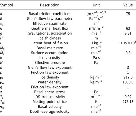
Table 1. Definitions and reference values of variables, parameters and constants in the model
Boundary conditions
At the glacier surface, temperature is prescribed as a Dirichlet boundary condition. We set temperatures to − 10° C at sea level with a lapse rate of − 0.007° C m−1 based on mean annual air temperatures (2013–2015) from the PROMICE weather stations in the vicinity of NEGIS (KPCL and KPCU, www.promice.org). As the surface elevation of the ice stream changes, so does the surface temperature following the lapse rate. Surface mass balance is applied uniformly with a value of $\dot {M}_{{\rm s}}=0.3$ m a−1, following MISMIP+ (Asay-Davis and others, Reference Asay-Davis2016). At the base of the ice the following Neumann boundary condition is applied in the thermal model:

The left side of the equation is the heat flux applied at the glacier bed, where k th is ice thermal conductivity, $\nabla T$ the temperature gradient and n the normal vector to the ice–bed interface. The right side is the GHF, G, and the frictional heat computed as the product of the basal velocity, vb, and basal drag, τb. GHF is temporally constant and uniformly distributed with a value of G =63 mW m−2, representing the average for the Greenland Ice Sheet (Rogozhina and others, Reference Rogozhina2012). The basal temperature is constrained to not exceed the melting point, and the excess heat is used to formulate the basal melt rate, $\dot {M}_{{\rm b}}$
 :
:
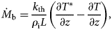
where L is the latent heat of fusion, ρ i the ice density, $T^\ast$ is the temperature computed before applying the constraints and T is the temperature after.
Boundary conditions for the stress balance model are as follows: at the ice divide there is a no-slip boundary condition, free-slip boundaries at the lateral margins (y = 0 and 80 km), and stress-free boundary conditions at the surface. No calving law is applied, instead ice is removed beyond x = 640 km as in the MISMIP + setup.
We use the default friction law in ISSM, with p = q = 1 in Eqn (3), reducing it to:

The friction coefficient α is spatially uniform and the value is based on a preceding study by Schlegel and others (Reference Schlegel, Larour, Seroussi, Morlighem and Box2015). From this study we computed our α as the mean value of their friction coefficient taken outside of the main trunk of NEGIS (velocities below 40 m a−1). Values for the parameters in the hydrology model were chosen to reach an overall mean floatation fraction of 0.7, similar to used for Russel glacier by de Fleurian and others (Reference de Fleurian2016), resulting in a 1 m thick sediment layer with transmissivity of T j = 0.02 m2 s−1. Other parameters in the hydrology set-up follow the one from the bf models in SHMIP (de Fleurian and others, Reference de Fleurian2018). The time step in the ice flow model is 1 year and for the hydrology model we use 1 day, both satisfying the Courant–Friedrichs–Lewy condition.
Experiments
The model was initialised and spun up for 100 ka to obtain a steady state with ice volume change less than 0.001% a−1 (Fig. 2). For the spin-up the masstransport, stress balance and the thermal solution were computed for all time steps, and the effective pressure computed every 5 ka. Temperature, velocity and thickness for the the initial state are shown in Figure 3. From this initial state we branch into two thermal steady-state simulations, with different GHF configurations (Fig. 2). In the first case we keep the same GHF configurations as the initial state (uniform G=63 mW m−2) and this becomes our Ctrl simulation. In the second case we force the model with a GHF anomaly computed by a mantle plume module in ISSM equal to Plume A in Seroussi and others (Reference Seroussi, Ivins, Wiens and Bondzio2017). The resulting GHF configuration is shown in Figure 1b, and has a maximum magnitude of 128 mW m−2, decreasing to similar values as the Ctrl simulation within 200 km. The GHF anomaly has a higher value than that suggested for North East Greenland by Grinsted and Dahl-Jensen (Reference Grinsted and Dahl-Jensen2002), Rogozhina and others (Reference Rogozhina2016), Rysgaard and others (Reference Rysgaard, Bendtsen, Mortensen and Sejr2018) and Dahl-Jensen and others (Reference Dahl-Jensen, Gundestrup, Gogineni and Miller2003), but similar to what Greve (Reference Greve2019) suggested for NGRIP, and much weaker than suggested by Fahnestock and others (Reference Fahnestock, Abdalati, Joughin, Brozena and Gogineni2001) and Alley and others (Reference Alley2019) (970 mW m−2).
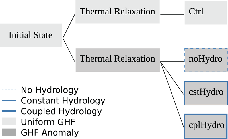
Fig. 2. Model flow chart for the control and three experiments. The leftmost box illustrates the initial state, which is the end of the 100 ka spin-up. The middle column represents the thermal relaxation step where the upper model is forced with a uniform geothermal heat flux like the initial state, and the lower model is forced with a geothermal heat flux anomaly, both in thermal steady state. The last column represents the control and the three different experiments. The control keeps both the GHF and the effective pressure from the initial state. The three experiments are forced with a GHF anomaly and differ by their degree of hydrological interaction with ice dynamics.
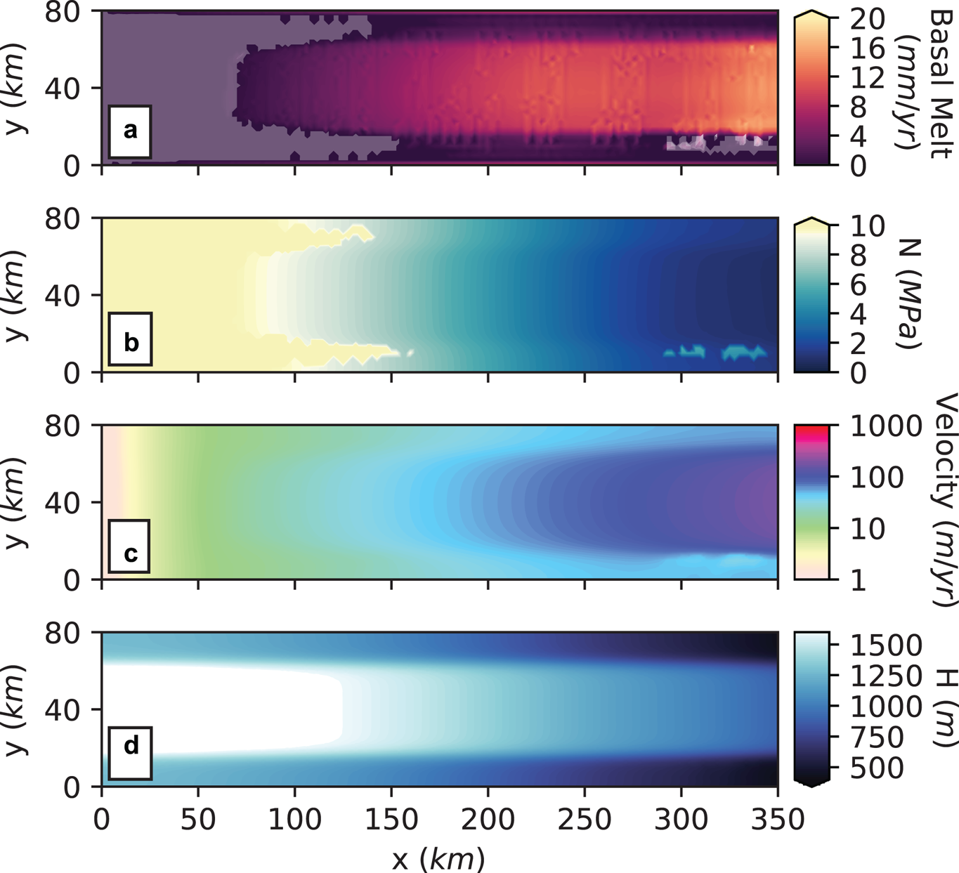
Fig. 3. Map view of key variables of the Ctrl simulation after 5 ka, ice flows to the right. Figure a shows basal melt rates, figure b effective pressure, figure c surface velocity and figure d ice thickness (H). Transparent masks indicate where the bed is below the pressure melting point. Note that we only show the upper 350 km part of the domain.
From the thermal steady state with the GHF anomaly we branch into three experiments (Fig. 2), which differ in their degree of the hydrological interaction with ice dynamics in the model simulation. In the first experiment (noHydro) we use the same effective pressure as in the Ctrl simulation, and change the thermal state. For the second experiment (cstHydro), we compute the effective pressure for the new thermal state and keep this field constant in time. In the third experiment (cplHydro) the subglacial hydrology model is offline coupled to the ice flow model. We use a loose coupling where a new hydrological steady state is recomputed every 500 years, to comply with the temporal evolution of both ice geometry and basal melt rates.
We use this gradual build up of complexity in our three experiments to disentangle the feedbacks and isolate the role of hydrology when investigating the influence of enhanced GHF on ice dynamics. In noHydro we study the effect GHF has on ice rheology alone. For cstHydro we introduce the hydrological effect and investigate the influence of GHF on sliding. Finally, in cplHydro we look into how the GHF influences the dynamics of the ice stream as hydrology and geometry interact, and positive and negative feedbacks arise.
As a sudden appearance of a GHF anomaly is not what we aim to investigate, but rather the influence of a permanent anomaly, we run all the experiments and the Ctrl simulation for 5 ka to reach equilibrium, and consider only the final time step. For cplHydro, it is challenging to reach true steady state, as this requires tight and computationally heavy coupling of the thermomechanical ice flow and the subglacial hydrology, which is not yet feasible in ISSM. Instead, we run the experiment until water pressure and ice thickness only show minor adjustments between two consecutive coupling steps.
Results
The impact of the elevated GHF, on both the dynamics and the thermal regime of the ice stream, differs between the three hydrology configurations. We first describe the Ctrl simulation, before presenting the response of the ice stream to the GHF anomaly in each of the experiments; noHydro, cstHydro and cplHydro.
Control (Ctrl)
In Figure 3 we present a map view of the key variables for the Ctrl simulation after 5 ka, for the upstream part of the domain. Note that we only show the upper 350 km of the domain, as we focus on how the GHF anomaly may influence the onset of the ice stream. Figure 3a shows the melt rates for the basal layer, with no melt at the ice divide and values increasing as we go downstream. Regions where the bed remains below pressure melting point are indicated with a transparent mask. This shows that a substantial part of the upper 150 km of the ice stream is cold based, in addition to a region downstream at the side of the trough. The corresponding effective pressure (Fig. 3b) confirms that the upper part of the domain is frozen, and thus displays effective pressure values equal to the overburden ice pressure. The effective pressure is decreasing downstream and reaches zero at the grounding line. The pattern in effective pressure results in slow velocity (Fig. 3c) at the ice divide and the fastest velocities at the grounding line. The ice stream is thickest at the centre of the trough with highest values at the ice divide and reaching the minimum thickness at the margins towards the grounding line (Fig. 3d). The ice stream is grounded at x = 400 km, 50 km further upstream than the original MISMIP+ experiments (Asay-Davis and others, Reference Asay-Davis2016). The geometry of the Ctrl run is plotted along the centre of the trough in Figure 7 (grey).
No hydrology (noHydro)
The introduction of an elevated GHF anomaly in the system without subglacial hydrology influences the basal thermal regime, but has a negligible dynamic impact. In Figure 4 we present the spatial differences between the noHydro and Ctrl simulations after 5 ka. We observe an increase in basal temperatures as the GHF anomaly is introduced, resulting in higher basal melt rates (Fig. 4a). The surface velocity above the GHF anomaly towards the ice divide remains unchanged (Fig. 4b). However, we observe a slow-down of the ice stream downstream towards the grounding line. The changes in velocity are relatively small, with a maximum of 1.3 m a−1 change in a region with surface velocity of 200 m a−1. The spatial pattern of the thickness variations show an overall lowering of the ice surface (Fig. 4c), with the largest changes directly above the GHF anomaly and reduced thinning downstream. The surface profile along the centre of the trough is shown in Figure 7 (light grey), and it falls on top of the Ctrl surface geometry, indicating minimal changes.
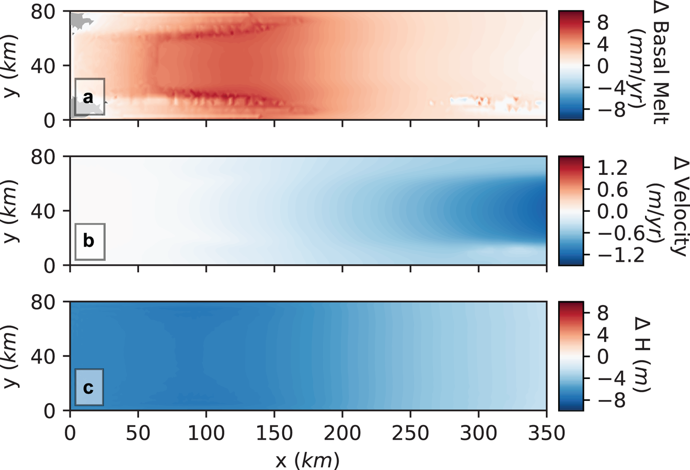
Fig. 4. Map view of the spatial impact of the GHF anomaly for the simulation without subglacial hydrology. Shown are the differences of the results (noHydro – Ctrl) at the end of the simulations for (a) basal melt rates, (b) surface velocity and (c) ice thickness. Grey region indicates where the bed is below pressure melting point.
Constant hydrology (cstHydro)
The influence of the elevated heat flux anomaly is more complex in the experiment with constant hydrology. In Figure 5 we present the spatial differences between cstHydro and Ctrl after 5 ka. We observe an increase in temperature in the GHF anomaly region, inducing higher basal melt rates (Fig. 5a). The increase in basal melt above the anomaly is 5.1 mm a−1, compared to 6.2 mm a−1 in noHydro (Fig. 4a). However, the ice stream displays a decrease in basal melt rates 100 km downstream of the GHF anomaly. Higher temperatures thaw the upstream part of the domain towards the ice divide, which is frozen in the Ctrl simulation, leaving only the margins of the ice divide still frozen (grey corners in Fig. 5b). The modifications in the basal melt field lead to major changes in the distribution of effective pressure (Fig. 5b), with a lowering of effective pressure all over the domain apart from the ice divide. The decrease is particularly apparent in the region that is frozen in Ctrl, and thawed in the cstHydro. The lowering of effective pressure leads to a speed-up of the ice stream (Fig. 5c), with a higher than 50 m a−1 increase in velocity, representing a 50% speed-up. The ice stream displays an asymmetric velocity pattern at the grounding line, caused by the frozen region at the margin (Fig. 3b, grey area). However, we observe a slow-down of the margins on each side of the maximum speed-up, inducing a more focused velocity pattern. The overall increased velocity causes a thinning of up to 400 m of the ice stream (Fig. 5d). The surface profile along the centre of the trough is given in Figure 7 (light blue), showing a flattening of the surface 100 km upstream of the grounding line, caused by the dynamic thinning.
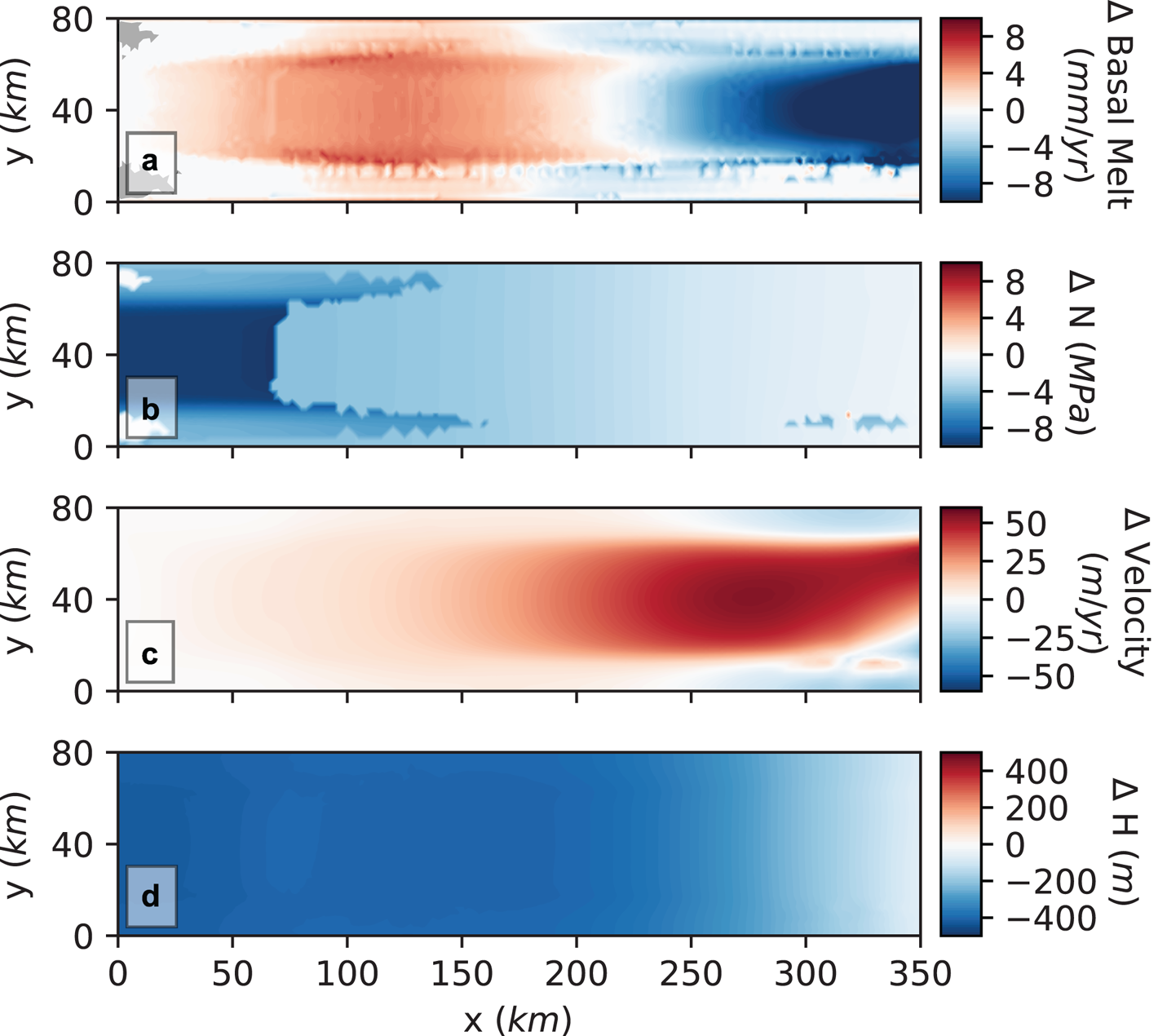
Fig. 5. Map view of the spatial impact of the GHF anomaly for the simulation with constant hydrology. Shown are the differences of the results with and without a geothermal heat anomaly (cstHydro – Ctrl) for (a) basal melt rates, (b) effective pressure, (c) surface velocity and (d) ice thickness. Grey region indicates where the bed is below pressure melting point.
Coupled hydrology (cplHydro)
The same GHF anomaly introduced in the coupled ice dynamic–subglacial hydrology system gives a less pronounced dynamic effect, relative to cstHydro. The impact of the GHF anomaly is presented spatially in Figure 6 as the difference between cplHydro and Ctrl after 5 ka. The increase of the GHF leads to an increase in basal melt rates of the same magnitude as in cstHydro, but extending further downstream (Fig. 6a). We observe a similar drop in effective pressure as in cstHydro (Fig. 6b), but a larger area of the domain remains frozen, stretching 50 km downstream from the ice divide at each margin (Fig. 6, grey area). As the effective pressure is lowered, the entire ice stream speeds up (Fig. 6c). However, the speed-up is lower in magnitude (average 24 m a−1) relative to the cstHydro simulation (average 42 m a−1), and we do not observe a slow-down of the margins. The resulting ice stream thickness shows a thinning compared to the Ctrl simulation, of up to 400 m (Fig. 6d). Relative to the cstHydro simulation, the thinning is of similar magnitude at the ice divide, but less widespread and diminishes towards the grounding line. The surface geometry along the centre of the trough is shown in Figure 7 (blue), and shows an overall flattening of the surface, caused by the thinning. The resulting surface is thus thicker and less steep compared to cstHydro (light blue).

Fig. 6. Map view of the spatial impact of the GHF anomaly for the simulation with coupled hydrology. Shown are the differences of the results with and without a geothermal heat anomaly (cplHydro – Ctrl) for (a) basal melt rates, (b) effective pressure, (c) surface velocity and (d) ice thickness. Grey region indicates where the bed is below pressure melting point.

Fig. 7. Surface profiles at the end of the experiments, plotted along the centreline of the ice stream. Surface of Ctrl is shown in grey, cstHydro in light blue and cplHydro in blue. The black line shows the base, with grounding line at x ≈ 400 km. Note, surface for noHydro falls on top of Ctrl. The vertical grey line indicates the position of the downstream boundary of Figures 3–6.
Discussion
Here we investigate the effect of including subglacial hydrology in the model and assess the influence of a local high in GHF on the dynamics and thermal regime of an ice stream. We find that geometric and dynamic changes in response to a local enhancement of GHF are significantly larger in the experiments with hydrology relative to without hydrology. When comparing the experiments including hydrology, the dynamic response to the GFH anomaly is more pronounced in the simulation with temporally constant hydrology (cstHydro) than in the simulation with interactive hydrology (cplHydro).
In the simulation without subglacial hydrology (noHydro), the dynamic influence of the GHF anomaly is small, as expected. On the other hand, the decrease in velocity downstream of the anomaly (Fig. 4b) is not expected. We explain this by higher basal melt rates in noHydro relative to Ctrl (Fig. 4a), leading to a thinning of the ice stream (Fig. 4c). The thinning induces a surface slope flattening, decreasing the driving stress (not shown), ultimately causing a slow-down of the ice stream (Fig. 4b). Counter-intuitively, instead of the elevated heat flux warming and softening the ice and enhancing the flow, the elevated heat flux causes a thinning and deceleration of the ice stream. This slow down occurs because the bed is already close to, or at, the pressure melting point before the GHF anomaly is introduced (Fig. 3a). We expect the results to be different if the extra heat applied, instead of mostly melting basal ice, increases the temperature of the ice column. Similar negative feedbacks with cold ice advection was recognised by Oerlemans (Reference Oerlemans1983) and Van Pelt and Oerlemans (Reference Van Pelt and Oerlemans2012) prohibiting further speed-up in their simulations.
Larour and others (Reference Larour, Morlighem, Seroussi, Schiermeier and Rignot2012a) investigated the impact of propagating GHF errors on ice hardness, and how this influenced mass flux in Pine Island Glacier. They concluded that, in fast flowing regions, a change of up to 50 mW m−2 in GHF only leads to a 1% change in the mass flux. Schlegel and others (Reference Schlegel, Larour, Seroussi, Morlighem and Box2015) did a similar study of the Northeast Greenland Ice Stream, and for the region with velocities closest to our simulations, uncertainty in GHF resulted in a minor change in mass flux. Pollard and others (Reference Pollard, DeConto and Nyblade2005) also concluded that a reasonable change in GHF had very little impact on ice dynamics. Similarly, the noHydro experiment shows a minor dynamic response to a doubling in GHF, and thus our findings agree with previous studies.
The inclusion of an elevated GHF anomaly in the constant hydro simulation (cstHydro) resulted in a substantial thinning and acceleration of the glacier. Velocity increases as a response to higher melt rates and drives the water pressure up, causing a reduction in effective pressure, and therefore lower basal drag (Fig. 5). The acceleration displays an asymmetric pattern towards the grounding line, which we explain by the downstream frozen area (Fig. 3, transparent mask). The asymmetric basal temperatures is caused by the anisotropic model mesh, leading to an asymmetric development of the efficient drainage system. Where the efficient drainage system activates, water pressure is reduced and velocity decreases, inducing less frictional heat. This causes one of the margins of the ice stream to freeze, and where basal melt rates are zero, the effective pressure is prescribed equal to the overburden ice pressure, thus leading to higher basal drag on one side of the ice stream. We acknowledge that this may be a numerical artefact as a result of the mesh resolution, this may change with a change in mesh resolution. For a prediction, or quantification study, using a realistic ice stream geometry, it is recommended to further refine the model mesh in fast flowing areas where the melt is high due to frictional heat. However, since this is a study of a synthetic ice stream with a focus on the upstream dynamic response to geothermal heat we find the model resolution sufficient.
Counter-intuitively, the ice stream cools in a region with accelerating ice flow, where one might expect warming due to an increase in frictional heat. The overall thinning may explain the observed cooling and reduced basal melt rates downstream of the GHF anomaly (Fig. 5a), as a result of less insulation and a change in the pressure melting point. Increased velocities also cause a draw-down of colder surface ice, cooling the ice column. The area around the GHF anomaly naturally does not cool, as this is compensated by the enhanced GHF. In the cstHydro simulation the surface temperature is fixed, despite changes in the surface height (in the cplHydro it is updated every 500 years). This influences the amount of heat advected and diffused towards the base. The observed cooling is thus overestimated, and the downstream cooling observed would be less pronounced if the surface temperature were to respond to changes in altitude.
The coupled hydrology simulation (cplHydro) displays an extensive dynamic response to the enhanced GHF: there is a significant thinning upstream, and the ice stream accelerates from the ice divide to the grounding line (Figs 6b,c). However, as hydrology is coupled to ice dynamics, and responds to changes in geometry (thinning), the resulting equilibrium state is thicker and flatter for cplHydro relative to cstHydro. As a consequence of the higher insulating effect of the thicker ice stream, cplHydro exhibits more extensive basal melt (Fig. 7). The downstream part of cplHydro cools similar to cstHydro, in an area where the GHF is minimally enhanced (Fig. 1). The less steep surface geometry of the ice stream in cplHydro, compared to cstHydro, results in smaller driving stress and reduced flow. Another reason why the cstHydro is showing a more pronounced speed-up than the cplHydro is the more extensive efficient drainage system in cplHydro (not shown). As a consequence, the water from the GHF anomaly is more efficiently evacuated away, resulting in higher effective pressure and thus a lesser increase in ice velocity in cplHydro.
The impact on velocity by the GHF anomaly in the runs including hydrology (cstHydro and cplHydro) is larger than observed by previous studies such as Larour and others (Reference Larour, Morlighem, Seroussi, Schiermeier and Rignot2012a) and Schlegel and others (Reference Schlegel, Larour, Seroussi, Morlighem and Box2015) involving ice streams with similar velocities. These studies do not include a hydrology model, and thus do not capture the influence from a change in basal drag. More importantly, their small sensitivities to GHF are largely due to ice velocities being highly sensitive to friction coefficients, which are inverted from observed surface velocities. Hence, most errors due to GHF are compensated by carrying out this inversion. These previous investigations showing small sensitivities of the mass flux in glaciers to GHF can be explained by neglecting subglacial hydrology. On the other hand, Pittard and others (Reference Pittard, Galton-Fenzi, Roberts and Watson2016a) used a simple hydrology model to capture the effect of regions with elevated heat flux and we expect their simulations to be similar to cstHydro. However, Pittard and others (Reference Pittard, Galton-Fenzi, Roberts and Watson2016a) do not observe a significant influence from the GHF anomaly in areas with similar velocity as our experiments. Despite a strong GHF anomaly (~3 times the background value), no melting occurs, thus the response they observe is mostly due to changes in the ice softness, similar to our noHydro experiment.
We observe a smaller thermal imprint of the GHF anomaly in the simulations with hydrology, compared to noHydro (Figs 4 and 6). Negative feedbacks arising with hydrological coupling have been recognised previously by Hoffman and Price (Reference Hoffman and Price2014), investigating the impact of a moulin in various hydrological configurations with increasing complexity. Similar decreases in temperature and thinning were observed by Gudlaugsson and others (Reference Gudlaugsson2017) when investigating the sensitivity of the Eurasian ice sheet to hydrology. They concluded that models without subglacial hydrology coupled to ice dynamics overestimated the area of temperate ice due to the exclusion of the negative feedback arising when water enhanced sliding advected cold ice downstream. Brinkerhoff and others (Reference Brinkerhoff, Meierbachtol, Johnson and Harper2011) found a diminishing sensitivity of the frozen/thawed boundary to increasingly higher GHF, and also concluded it to be due to the inability to overcome cold advected ice from upstream.
The subglacial hydrology drainage system of fast flowing ice is difficult, or even impossible to observe, thus leaving the hydrology model parameter space highly uncertain and unconstrained. The conductivity of the drainage system impacts the efficiency in evacuating water and therefore controls the sensitivity of the system to water input. With a lower conductivity, the dynamic response to the GHF anomaly will be enhanced, as the same water input will in this case result in a higher water pressure and hence reduced friction. A change in both the sediment thickness and transmissivity would therefore impact our results. We expect the hydrology system close to the ice divide of an ice stream to be inefficient with low conductivity, therefore the model may underestimate the dynamic response of the ice stream to the GHF anomaly.
In this study we use a simple friction law where basal drag depends linearly on the effective pressure. The friction law is a crucial link between the subglacial hydrology and the ice dynamics, and a different choice of friction law would likely change our results. Particularly, the friction law used in the MISMIP+ experiments (Asay-Davis and others, Reference Asay-Davis2016; Tsai and others, Reference Tsai, Stewart and Thompson2015) includes effective pressure only where the coulomb criterion is met, usually near the grounding line. This friction law would hence give a less dynamic response to the upstream changes in effective pressure from the GHF anomaly observed in our experiments. Therefore, by using a simple friction law we may overestimate the sensitivity of the ice stream to GHF anomalies. Unfortunately, defining a universal friction law remains one of the biggest challenges in glaciology.
In the cplHydro experiment, we use a coupling with a relatively long coupling time of 500 years, where the hydrology model is run to steady state for every coupling step. After 5 ka, we reach two consecutive coupling steps in which neither water head, nor the ice geometry changes significantly. We still observe minor oscillations in ice geometry between the coupling steps, however the changes are small relative to the preceding coupling steps and the differences between the three experiments. We therefore find this loose coupling approach sufficient to serve the purpose of this paper. Coupling thermomechanical ice flow models to sophisticated subglacial hydrology models is in its infancy, and future studies should focus on how to fully couple these models and investigate how coupling time influences ice dynamics and oscillations.
Including subglacial hydrology models computing the effective pressure in ice flow models will have implications for future GHF studies in regions where the bed is at the pressure melting point. Our results imply that previous studies may have underestimated the sensitivity of ice flow to elevated heat flux, and overestimated the influence on basal melt rates, by excluding subglacial hydrology. The negative feedbacks arising by the inclusion of subglacial hydrology may be of particular interest for studies like Greve (Reference Greve2019), using ice flow models to constrain GHF values by matching modelled basal temperatures to observed ones. As GHF maps become less uncertain and more detailed, and in order to capture the impact of this, effective pressure must be included in the friction laws of ice flow models. This is particularly important for studies predicting future ice-sheet behaviour where one cannot invert for basal drag, as surface velocity observations do not exist and basal drag is thought to change with a changing climate.
Including effective pressure in friction laws will help resolve the complex flow patterns observed in the Greenland Ice Sheet (Beyer and others, Reference Beyer, Kleiner, Aizinger and Humbert2018). The increase in velocity in both our cstHydro and cplHydro experiments agree with the hypothesis that NEGIS and other ice streams may be initiated by elevated GHF anomalies (Fahnestock and others, Reference Fahnestock, Abdalati, Joughin, Brozena and Gogineni2001; Rogozhina and others, Reference Rogozhina2016; Alley and others, Reference Alley2019). At present, ice-sheet models are not able to reproduce the characteristic upstream flow pattern of NEGIS (Goelzer and others, Reference Goelzer2018). Including a local GHF anomaly and a subglacial hydrology model is the key to solve this in future studies.
Conclusions
We have investigated the impact of using a subglacial hydrology model on the dynamic and thermal response of an ice stream to elevated geothermal heat flux. Our results indicate that ice streams are more sensitive to GHF than previously shown in studies excluding the impact on effective pressure. With a locally enhanced GHF, we find increased velocities and substantial thinning of the ice stream, and the effect is significantly larger in experiments including subglacial hydrology. We observe an insignificant dynamic impact of GHF in the experiment without hydrology, despite the melt rates being higher. This suggest that previous studies excluding hydrology may have underestimated the dynamic and overestimated the thermal effects. On long time-scales, the coupled ice dynamics–hydrology system shows a dampened response to the elevated GHF anomaly, due to the negative feedbacks hindering the expected warming and speed-up. Including subglacial hydrology in models may help to reproduce the observed complex velocity pattern in ice sheets, particularly the NEGIS, suggested to be induced by highGHF.
Contribution statement
The study was designed and developed by the three authors. SSJ performed the simulations and wrote the paper with contributions from BdF and KHN.
Acknowledgments
SSJ, BdF and KHN have received funding from the European Research Council under the European Community's Seventh Framework Programme (FP7/2007–2013) ERC grant agreement 610055 as part of the ice2ice project. BdF received funding from Bjerknes Centre strategic project RISES. The computations were performed on resources provided by UNINETT Sigma2 – the National Infrastructure for High Performance Computing and Data Storage in Norway (nn4659k and nn9635k). We thank Nicole Schlegel for inspiration and help with ISSM and Helene Seroussi for providing her MISMIP+ set-up in ISSM and for support with ISSM. Finally, we thank Andy Aschwanden and one anonymous reviewer for greatly improving the manuscript.


 Open access