


1. Introduction
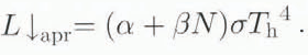
This paper concerns the parameterization of the incoming longwave radiation L ↓ above a large ice sheet under conditions with surface melting. Such a parameterization is required for models to investigate the response of the Greenland ice sheet to global warming. In principle, L ↓ can be determined fairly accurately from profiles of temperature (T), water-vapour density (ρ v) and liquid or solid water density. However, it is often assumed that L ↓ can be expressed in terms of parameters at the reference height (h), as
in which Th, is the absolute temperature at the reference height, σ is the Stefan – Boltzmann constant and εeff is the effective emittance. Empirically, εeff is found to be a function of cloudiness (N), water-vapour density at the reference height (ρ vh) and also of the geographical location. The dependence on location is caused by systematic differences between the profiles and cloud properties, as well as by differences in surface elevation.
The parameterization (Equation (1)) is used in glaciology for several purposes. It has often been applied to evaluate L ↓ for field campaigns in which N, T h, and vh have been observed but L ↓ has not. Recently, Equation (1) has also been used in model studies related to the response of the Greenland ice sheet to climate change. In those studies, L↓ is determined from a prescribed, idealized temperature series. Reference Greuell, and KonzelmannGreuell and Konzelmann (1994) applied this parameterization to estimate the yearly energy balance for one site (ETH Camp, southwest Greenland), with ρeff as determined by Reference Konzelmann,, van de Wal, Greuell, Bintanja, Henneken and Abe-Ouchi,Konzelmann and others (1994) from measurements at the same site. Reference Van de Wal, and OerlemansVan de Wal and Oerlemans (1994) used it to perform yearly energy-balance calculations for the whole Greenland ice sheet. More research along this line is expected in the near future.
Though the validity of Equation (1) has been rather well confirmed for typical cases such as ordinary land surfaces during the daytime, it has not been so for glaciers where melting occurs. There is a particular difficulty with such surfaces. As the air temperatures rise, the glacier surface remains at the melting point and hence the temperature rise cannot be uniform with height. It should be expected then that the rise in T h is smaller than the rise in the temperatures above. Since the latter also yield a contribution to L ↓, L ↓ rises faster than T h 4, so that εeff is a rising function of Τ h.
Actually, it is well known that large errors would occur for melting mountain glaciers, for which the T profiles are obviously perturbed by advection of air from the ice-free surroundings. For such glaciers, it is obvious that Equation (1) cannot be applied with a T h measured above the glacier. Reference Greuell,, Oerlemans and Oerlemans,Greuell and Oerlemans (1989) calculated L ↓ from a T h measured at a site beyond the thermal influence of the glacier, whereas Reference Kuhn, and Oerlemans,Kuhn (1989) used a weighted average of T h 4 beyond the influence of the glacier and above it. For large ice sheets without advection from ice-free surroundings, the matter is different. The use of Equation (l) for that case is based on the assumption that the atmosphere will adapt to the surface conditions up to a sufficient height, so that T h, is “representative” (Reference Greuell,Greuell, 1992).
In earlier papers, attempts have been made to evaluate the validity of Equation (1) from data that were acquired on the Greenland ice sheet. Reference Greuell,Greuell (1992) investigated the dependence of εeff on Τ h for the ETH Camp (see above) and found that it could not be determined whether εeff was dependent on or independent of T h, due to the large scatter of εeff. He recalled an interesting result from Reference Ohmura,Ohmura (1981), who found from a long sequence of data, taken on Axel Heiberg Island (this concerns a smaller ice cap), that εeff is an increasing function of T h. Reference Konzelmann,, van de Wal, Greuell, Bintanja, Henneken and Abe-Ouchi,Konzelmann and others (1994) also found a large scatter in εeff. Another problem is that Equation (1) has not been tested for the ablation zone, where the highest air temperatures above the ice sheet are found.
A theoretical test has also been tried. Reference Konzelmann,, van de Wal, Greuell, Bintanja, Henneken and Abe-Ouchi,Konzelmann and others (1994) calculated L ↓ with a narrow-band model from profiles of T and ρ v. Standard profiles were chosen, based on inspection of radio soundings, and then ρ v and T were varied by amounts that did not depend on height. This yielded good accord with Equation (1). However, a crucial flaw in this numerical experiment is that the boundary condition for a melting glacier was not incorporated, so that there is a systematic difference between the idealized profiles of the experiment (which differ mutually by an additive constant) and the real profiles (which differ the more, the greater the height becomes), once melting occurs.
In the present paper, the usefulness of Equation (1) for the lower part of the Greenland ice sheet is evaluated. This is done in two ways. First, the relation between observed values for T h 4, and L ↓ is investigated for a location on a melting surface where a large range of positive T h, values occurs. It is noted here that such measurements have rarely been done, which is to be attributed primarily to the experimental difficulties involved in performing measurements over an ice surface with a high melting rate (Reference Oerlemans, and VugtsOerlemans and Vugts, 1993). Secondly, a case study with a numerical meso-scale model is analysed, in which the change of the T profile is calculated from the changes in air flow and turbulence, which in their turn depend on the temperature difference between air and atmosphere (Reference Meesters,Meesters, 1994). If the difference with Equation (1) is large, it should be concluded that parameterizing L ↓ along this line is inappropriate in a model to study the reaction of a large ice sheet in climate change.
2. Observations
2.1. Site and Set-Up of the Observations
A general description of the Greenland Ice Margin Experiment (GIMEX) can be found in Reference Oerlemans, and VugtsOerlemans and Vugts (1993). A more detailed description of the climate of the ablation zone can be found in Reference Van den Brocke,, Duynkerke and OerlemansVan den Brocke and others (1994). Several papers on GIMEX have been published in a special issue of Global and Planetary Change (No. 9, 1994).
During GIMEX-91. radiation data were collected during 52 d, 10 June – 31 July 1991. In this study, we will use data collected at “site 4” on Russell Glacier, 2.5 km from the boundary between glacier and tundra at an elevation of 340 m a.s.l. Fig. 1). These measurements were performed by the Institute for Marine and Atmospberic Research, University of Utrecht. Advection of warm air from the tundra plays no role at this site, at least at the lower heights, as is shown by the very high directional constancy (0.97) of the east-southeast wind (Reference Van den Brocke,, Duynkerke and OerlemansVan den Brocke and others, 1994). The glacier surface at this location is very rough: the regularly spaced ice hills (formed by mechanical deformation and differential melting) have typical dimensions of several metres vertically and horizontally. This and the high seasonal melt rate (3.1 m water equivalent; Reference Van de Wal,Van de Wal and others, 1995) prevents the operation of tall masts and sensitive equipment. Instead, we used a 6 m mast that rested freely on the ice with its four legs and melted down with the surface in the course of the ablation season.

Fig. 1. Location of the site (“site 4”) from which observations were used.
At 1.5 m above the surface, shortwave radiation was measured with Kipp CM 14 pyranometers and total radiation with Aanderaa 2811 pyranometers. As these sensors were not ventilated, the measurements were perturbed by heating of the sensor housing due to insolation. After the experiment, all the radiation sensors were recalibrated and several corrections were applied before the data could be analysed. Since longwave radiation was not measured directly, it was calculated by subtracting the global from the total radiation. This procedure, together with the typical measuring accuracy of the sensors, yields an estimated accuracy of the measured daily mean incoming longwave radiation L ↓ of 10 W m−2.
Temperature and humidity were measured at three levels. In this paper, only temperature and humidity measurements at h = 2 m are used.
2.2. Results and Comparison with Theory
Only diurnal means have been used for comparison with theory to minimize the influence of errors in the measured radiation and in the observed cloudiness. The diurnal course of the temperature at the reference height. T h, is small so that the average of the fourth power of T h can be estimated as the fourth power of the average of T h.
A problem is that the incoming radiation depends strongly on the cloudiness N, even if N is small. In Fig. 2 the observed εeff shown as a function of N only. A linear dependence is seen. This behaviour differs strongly from other results for polar regions (Reference König-Langlo, and AugsteinKönig-Langlo and Augstein, 1994; Reference Konzelmann,, van de Wal, Greuell, Bintanja, Henneken and Abe-Ouchi,Konzelmann and others, 1994), which are also shown in Fig. 2. According to those results, the cloud contribution is about proportional to the third power of N. Reference Konzelmann,, van de Wal, Greuell, Bintanja, Henneken and Abe-Ouchi,Konzelmann and others (1994) explained this by remarking that, in the case of low N, only high cirri are present, which have a small influence on L ↓, whereas high N is related to clouds with a low base. This rule apparently does not hold for the GIMEX site 4. For a clear sky, however, there is a good agreement between the observations for site 4 and the two parameterizations.

Fig. 2. Observed atmospheric emittance on cloudiness, for “site 4”, June – July 1991. Also shown are two parameterizations, based on measurements at other polar sites (equilibrium line of southwest Greenland in the case of Reference Konzelmann,, van de Wal, Greuell, Bintanja, Henneken and Abe-Ouchi,Konzelmann and others (1994) and Koldewey (Svalbard) and Georg von Neumayer (Antarctica) in the case of Reference König-Langlo, and AugsteinKönig-Langlo and Augstein (1994)).
A straightforward way to account for the influence of the clouds, starting from the assumed proportionality of L ↓ to T h 4, is to assume that the following approximation can be used:
The best values for α and β have been determined from L↓obs, N and T h by a least-squares calculation. It was found that α = 0.78 ± 0.01 and β = 0.14 ± 0.01, with a high correlation of r αβ = – 0.8. In Fig. 3, L ↓. as determined by Equation (2) is compared to the observed L ↓. The correlation between the observed and explained L ↓ is rather high, r xy = 0.88, suggesting that the model is good. However, things become different if one looks at the predictions for dependence on T h for fixed N. To do so, the data points have been classified according to N being “low” (N ≤ 0.3), “moderate5 (0.3 < N ≤ 0.7 and “high“ N > 0.7. In Fig. 3, the data points have been marked accordingly. The least-squares linear fit for each class is also shown. The slopes of these fits appear to be 0.50 ± 0.11 for Low N, 0.39 ± 0.10 for moderate N and 0.24 ± 0.26 for high N. All slopes are significantly smaller than 1. This indicates than L↓obs rises considerably faster than T h 4 for fixed N, so that Equation (2) and hence Equation (1) are refuted for this case. We have not tried to obtain a better relation, since it would be impossible to generalize it to cover a larger area as the observations have been done at a rather special location. It is emphasized that the noted discrepancy cannot be explained, as for small glaciers, by advection of warm air from the snow-free surroundings, since the surface wind was always from the ice sheet as noted in section 2.1. In the following section it will be shown that this discrepancy is likely to occur for the whole area where melting is important.

Fig. 3. Observed as calculated incoming longwave radiation for “site 4”. Three classes for cloudiness (N) have been discerned. The solid lines are the best linear fits for the three classes.
3. Numerical Calculations
3.1. Set-Up of the Numerical Calculations
A two-dimensional meteorological meso-scale model has been used; this was developed to study the relation between the atmospheric circulation and the surface-energy balance for the western margin of the Greenland ice sheet. The model has been described and validated by Reference Meesters,Meesters (1994) and Reference Meesters,, Henneken,, Bink,, Vugts and CannemeijerMeesters and others (1994). Only those features that are most important for the present paper are briefly reviewed.
Figure 4 indicates the topography in the model. A terrain-following staggered grid is used. There are 13 levels for the temperature above the surface, with the lowest heights at 10, 20, 40, 80, 120 m and the highest level at 5000 m. No clouds are assumed to be present. L ↓ is parameterized at the surface altitude z sur according to

in which ε(zsur , s) is a function of the water-vapour content between zsur and s, parameterized according to the suggestion of Reference Savijärvi,Savijärvi (1990).

Fig. 4. Topography used for the two-dimensional meso-scale model.
3.2. Results of the Numerical Calculations
Two runs ( A and B) with the model will be considered here. They correspond to runs A and C discussed by Reference Meesters,Meesters (1994). Run A is a standard run with a clear sky. no large-scale wind and temperature, moisture and ice conditions representing a day in July. Run B differs from run A only in that the initial air temperature is increased by 5 K at all levels. This causes large differences in the wind field and in the turbulent exchange, as has been discussed by Reference Meesters,Meesters (1994). Both runs started at midnight and lasted for 48 h. In this section, averages for the latter of the 2 d are considered.
Figure 5 shows the diurnally averaged temperatures, at the surface and at the reference height (10 m), for both runs. It is seen that the difference between both runs is small for small x and increases with increasing altitude. Yet, for the highest altitude (x=400 km), the increase is still considerably smaller than the imposed rise of the free-atmosphere temperature, 5 K.

Fig. 5. Surface (Ts) and reference height (Th) temperature for runs A (solid) and B (dashed). Daily averaged values, as a function of the distance to the ice margin.
These features have the following background. Close to the ice margin, the average air temperatures are high due to the low altitude. Surface melting inhibits large differences between runs A and B. With increasing altitude, temperatures generally become lower. At the highest altitude, melting occurs only during a small part of the day for run A but during a considerable part of the day for run B (Reference Meesters,Meesters, 1994). Hence, the difference between the mean temperatures for runs A and B at high altitude is, although much higher than for low altitudes, considerably smaller than the difference of 5 K imposed on the free-atmosphere temperature.
Figure 6 shows the diurnal averages for the temperature profiles for both runs, for three locations. Locations “L” and “H” are at the foot and at the top (surface elevation 2.5 km) of the slope, respectively, and location “M” is at x = 90 km, for which the surface elevation is 1.2 km. This figure illustrates that suppression of the temperature rise, which occurs for the “warm” part of the ice sheet, is restricted to a shallow layer. Figure 7 shows the relative increase, from run A to run B, of L ↓ as well as T h 4. It is seen that for the “warm” part of the ice sheet, the increase of L ↓ for clear-sky conditions is underestimated by a factor of up to 3 if one applies Equation (1)

Fig. 6. Temperature profiles for sites with a low (L), middle (M) and high (H) altitude, for runs A (solid) and B (dashed). Daily averaged values.

Fig. 7. Increment of the incoming longwave radiation (L ↓) and of the fourth power of the temperature at reference height (Th 4). Daily averaged values as a function of the distance to the ice margin.
The difference cannot be explained from the change in water-vapour content ρ
vh. Inspection shows than ρ
hw, increases by only 5% from run A to run B, averaged over the zone ![]() . But since (for clear sky and with changes in the shapes of the profiles neglected) εeff should be proportional to a low power of ρ
vh (power T
h
4 according to Reference Konzelmann,, van de Wal, Greuell, Bintanja, Henneken and Abe-Ouchi,Konzelmann and others 1994), this can explain a change of less than 1% in εeff. Hence, the noted change in L ↓ has to be attributed for the greater part to the systematic change in the shapes of the profiles.
. But since (for clear sky and with changes in the shapes of the profiles neglected) εeff should be proportional to a low power of ρ
vh (power T
h
4 according to Reference Konzelmann,, van de Wal, Greuell, Bintanja, Henneken and Abe-Ouchi,Konzelmann and others 1994), this can explain a change of less than 1% in εeff. Hence, the noted change in L ↓ has to be attributed for the greater part to the systematic change in the shapes of the profiles.
The apparent shallowness of the layer that is adapted to the surface cannot be a consequence of the limited simulation time (2 d). A katabatic wind flows over Greenland with a typical length scale of 500 km and a speed (coastward component) of 5 m s−1, yielding a time-scale of only 105 or about 1 d.
4. Discussion
The assumption that the incoming (clear-sky) longwave radiation L ↓ should be roughly proportional to the fourth power of the temperature at the reference height T h 4 has been tested for the Greenland ice sheet. It has been found, both from observations and from simulations, that in response to a large-scale warming a rise in L ↓ occurs which is much larger than the rise in T h 4 for those sites where melting occurs during a large part of the day. This is explained from the fact that T h is kept low by the melting surface, whereas L ↓ rises more strongly since the temperatures at higher levels also contribute to L ↓. The existence of this effect was known beforehand but it has usually been considered as negligible. The present study has shown that this is in general not the case.
It is emphasized that even relatively small errors in the calculation of L ↓ lead to large errors in the net radiation if the latter is small. This is the case for the Greenland ice sheet during the melting season, when the net longwave radiation and net shortwave radiation tend to cancel because of the high albedo of the ice (e.g. Reference Van de Wal, and OerlemansVan de Wal and Oerlemans, 1994). Hence, studying the response of the ice sheet to climate change requires an accurate parameterization of L ↓.
Equalion (1) has rarely been applied to cases with high air temperatures over melting glaciers. However, Reference Van de Wal, and OerlemansVan de Wal and Oerleinans (1994) used Equation (1) in a model for the response of the Greenland ice sheet to climate change. They stipulated the effect of climate change by increasing the air temperature T h by 1 K everywhere. Since the effect of surface melting on T h has not been taken into account, it is likely that the calculated increase in L ↓ would be relatively well in accord with the stipulated climate change, whereas the prescribed increase in T h, itself would not be. So, the effects of a wrong T h and a wrong relation between T h and L ↓ cancel (whereas, on the other hand, the turbulent fluxes will be calculated wrongly to the extent that T h is wrong but this problem is beyond the scope of the present study).
It is concluded that the use of Equation (1) in models to simulate the response of ice sheets to large-scale warming leads, as far as the equation is taken literally, to a strong underestimation of the change in the incoming longwave and net radiation once surface melting occurs. For this reason, the use of models with several T levels within the atmosphere is strongly recommended.
Acknowledgements
We thank the members of the GIMEX-91 team for their participation by undertaking the measurements at site 4. P. G. Duynkerke. W. Greuell, J. Oerlemans and R. S. W. van de Wal (Institute of Marine and Atmospheric Sciences, Utrecht) are thanked for helpful discussions. Financial support was obtained from the Dutch National Research Program on Global Air Pollution and Climate Change (contract 276/91-NOP), from the Commission of the European Communities (contract EPOC-CT90-0015) and from the Netherlands Organisation for Scientific Research (Werkgemeenschap CO2-Problematiek).


