


Introduction
In the past, theoretical treatments (Reference MarchiMarchi, 1895; Reference FinsterwalderFinsterwalder, 1907; Reference NyeNye, 1958, Reference Nye1960, Reference Nye1961, Reference Nye and Kingery1963; Reference WeertmanWeertman, 1958) of nonequilibrium glaciers and ice sheets have been concerned primarily with the effect of small perturbations from a stable equilibrium state. An interesting problem which lies outside the scope of such theories is the determination of the time required for a small, nonequilibrium ice cap to grow into a large, stable ice sheet. This determination is of practical importance in the study of the chronology of the Pleistocene Epoch. A knowledge of the growth time of an ice sheet is valuable in any theoretical consideration of the cause of ice ages. For example, if it were found that the time required to build up an ice-age sheet is of the order of the duration of one glacial stage or substage, this fact would lend support to any theory in which the growth of an ice sheet triggers off the mechanism which ultimately causes the destruction and disappearance of the ice sheet.
Perturbation-type theories have shown that the behavior of nonequilibrium glaciers and ice sheets is complex. As an illustration we may note that the mathematical equation which predicts the time-dependence of a perturbation contains a diffusion term, an exponential time term, and a term which is associated with the occurrence of traveling waves. It is reasonable to expect the same complex behavior in an ice sheet which grows from a small to a large size (or contracts from a large to small area). Obviously, it would be difficult to develop a theory which describes in detail this complicated response of ice sheets to nonequilibrium conditions. Moreover unless the fine details of the growth process are of interest, it is unnecessary to develop a complete theory in order to obtain the time required by a small ice sheet to become large. In the following sections we present a more modest theory which gives growth and shrinkage times but which does not attempt to investigate such problems as kinematic waves or kindred phenomena involved in the nonequilibrium behavior of glaciers and ice sheets.
Basis of Theory
The reader may recall that the modern theory of glacier mechanics started with the calculation by Reference OrowanOrowan (1949) of an ice sheet profile. His calculation was based upon the assumption of perfect plasticity, i.e. it was postulated that no plastic deformation can occur in a solid until a certain stress, τ 0 is exceeded. At this stress level there is an infinite amount of deformation. Thus the solid cannot support a stress larger than τ 0 Orowan’s work was greatly extended by Reference NyeNye (1951), who still used the theory of perfect plasticity as the basis of his calculations. His work showed that the use of this theory is a reasonable approach to glacier mechanics. In fact the observed and calculated profiles of the Unteraar Glacier are in remarkable agreement (Reference NyeNye, 1952).
The application of perfect plasticity to glacier mechanics was abandoned after the experimental work of Reference GlenGlen (1955) on the creep of ice provided a more realistic plastic deformation law. He found the following creep law for ice
where
Profiles (Reference NyeNye, 1959; Reference WeertmanWeertman, 1961) of ice sheets which were calculated with the aid of Glen’s creep law are similar to those found using the perfect plasticity deformation law. This result is not surprising. The perfect plasticity deformation law is a fair approximation to equation (1). Figure 1 is a schematic plot of stress versus creep rates given by equation (1) for various values of n. Setting the value of n equal to infinity produces the curve of a perfectly plastic solid. This curve approximates the curve of n = 3, which describes the actual behavior of ice.

Fig. 1. Schematic plot of stress versus creep rate for n = 3, n = 9, and n = ∞. The last value corresponds to perfect plasticity
In addition to the similarity in profiles, other results of perfect plasticity theory are close to those found in the more realistic glacier mechanics theory. In the perfect plastic case it is found that the shear stress acting at the bottom of a glacier and parallel to its bed is a constant. (Its value is taken to be 1 bar.) In the more exact theory the shear stress at the bed is not constant, but the variation in the value of the stress is relatively small. (The spread is from about 0.5 to 1.5 bars.) To a first approximation the stress may be considered constant. According to the perfect plastic theory the thickness at the center of an ice sheet of given width is independent of the accumulation rate. In the more exact theory the thickness does depend on accumulation rate but the dependence is extremely weak. The thickness depends on the accumulation rate only to a
The perfect plasticity theory is inadequate for the investigation of such phenomena as kinematic waves. These can be handled only by the more exact theory. However, as was mentioned in the introduction, we actually wish to avoid a detailed examination of this type of complicated phenomenon. The possibility arises therefore that the shortcomings of the abandoned perfect plasticity theory can be turned to advantage for us. It automatically masks the glacier phenomena we do not want to see. In the analysis which follows it will be assumed that the behavior of ice may be described by letting n of equation (1) approach infinity.
Basic Equations
The equations basic to our analysis can be set up with the aid of Figure 2. This figure shows the cross section of one half of an ice sheet resting on a flat base. The ice sheet extends over an infinite distance in the direction perpendicular to the plane of the paper. At a distance x from the center of the ice sheet the thickness of the ice is equal to h. The average velocity of the ice passing through a vertical plane at x is V. The average accumulation at x, converted to the equivalent amount of high density ice, is a. The accumulation has the units of volume of ice per unit surface of the ice sheet. The accumulation rate may be a function of the distance x. A positive value of a corresponds to accumulation and a negative value to ablation.

Fig. 2. Cross section of one half of an ice sheet which rests or a flat base. The ice sheet extends an infinite distance in a direction perpendicular to the plane of the paper
When the ice sheet is in a nonequilibrium state the value of h will not be constant. An expression for its time variation may be obtained from a consideration of the mass budget between the vertical planes at x and x + δx Per unit time, the amount of ice passing across the plane x is Vh and across x + δx is Vh + [∂(Vh)/∂x]δx. The difference in the flow of ice across the two sections is [∂(Vh)/∂x]δx. The accumulation at the upper surface increases the height by the amount aδx (Any possible loss or gain at the bottom surface will be neglected.) If h is not constant the volume of ice between the two vertical planes will change by an amount (∂h/∂t)δx throughout this pc. From the requirement of the conservation of the volume of ice (ice is assumed to be incompressible taper) we obtain the equation
The theory of glacier mechanics based on equation (1) gives the following approximate expression for the average velocity V 0
where τ is the shear stress acting at the bed of the glacier and V 0, τ 0, and m are constants. The value of m differs somewhat from the previously used n. The magnitude of the difference depends on the relative values of the contributions to V from sliding at the bottom and from the creep deformation within the ice sheet. For our purposes it is necessary only to note that if the value of n approaches infinity the value of m likewise approaches infinity. Observations on glaciers which have a shear stress τ at the bed of about 1 bar indicate that the velocity V is approximately 100 m./yr. Thus, if τ 0 is taken to be equal to 1 bar, 100 m./yr. is an appropriate value for V 0.
To a good approximation the shear stress acting at the bottom of a glacier is given by
where ρ is the density of ice and g is the gravitational acceleration. The minus sign is used in this equation so that τ will be a positive quantity.
By inserting equations (3) and (4) into equation (2) we obtain
Equations (2) and (5) may be integrated with respect to x at any given instant in time:

This equation can be rewritten as

Consider now the perfectly plastic case in which m is allowed to approach infinity. If the values of a and ∂h/∂t are nonzero, the following conclusions are obvious:
-
I.
(7a)
-
II.
(7b)(Except in unusual situations, this equation reduces to a = ∂h/∂t)
-
III. The right-hand side of equation (6a) can never have a negative value,
-
IV. Any state of an ice sheet for which τ>τ 0 can last only an infinitesimally small length of time.


We need consider only the two conditions given by equations (7a) and (7b). These equations will be of great importance to our analysis. The nonequilibrium ice sheets in which we are interested contain both accumulation and ablation areas. In order to understand the behavior of these ice sheets it is instructive to consider first the simpler case of ice sheets which contain only accumulation areas or only ablation areas.
Growing Ice Sheets which contain only an Accumulation Zone
Let us consider the case of an ice sheet which rests on a flat base. This ice sheet extends an infinite distance in the horizontal direction. Suppose that there is no ablation zone on the ice sheet. Suppose further that the rate of accumulation does not depend on the distance x but that accumulation occurs only on the ice sheet itself and not on the exposed, ice-free, ground. We would expect that for this ice sheet equation (7a), which predicts that the shear stress at the bed is equal to τ 0, is valid. (If the shear stress at the bed of the ice sheet were less than τ 0 over an extensive area, the ice in this region would be stagnant and not flow. From equation (7b) it can be seen that in this stagnant area the ice thickness builds up at the rate ∂h/∂t = a. Eventually the ice thickness will become large enough to make the shear stress τ equal τ 0.) From equation (4) we find that
which integrates to
where
In these equations, which were found first by Orowan, H is the thickness of the ice sheet at its center and L is its half-width (Fig. 2).
Because there is no ablation area on the ice sheet the total volume of the sheet must increase. It can be seen that for one half of an ice sheet, such as shown in Figure 2, the rate of increase of volume per unit length is simply aL. (The unit length is measured in the direction perpendicular to the plane of the drawing.) The total volume of ice per unit length of one half of the ice sheet is

Thus the rate of change of the volume is equal to
which integrates to
where t is the time required for an ice sheet of initial half-width L o to grow to a half-width L. Figure 3 shows plots of accumulation rate versus the time required to build an ice sheet up to a half-width L = 1,000 km. when L 0 ≪ L. The value L = 1,000 km. is of the order of the half-width of ice-age ice sheets. The curves of Figure 3 are calculated assuming τ 0 = 1 bar and τ 0 = 0.5 bar. (The former value gives H = 4.8 km. and the latter H = 3.4 km.)

Fig. 3. Double log plot of the growth or shrinkage time of an ice sheet of half-width L = 1,000 km. as a function of accumulation or ablation rate. Solid lines: time required for build up; dashed lines: time required for disappearance. Equations (13) and (16) of the text were used to obtain these lines. The hatching indicates reasonable accumulation or ablation rates for growing or shrinking ice sheets
Shrinking Ice Sheets which contain only an Ablation Zone
Suppose now that the supply of ice producing accumulation on the growing ice sheet of the previous problem is turned off and instead there is ablation over the entire surface. A volume of ice aL, where a has a negative value, is now removed from the glacier.
The rate of shrinkage of the ice sheet cannot be found simply by reversing the analysis of the previous section. In that situation, because of accumulation, the ice sheet would maintain a profile such that the shear stress at the bottom is −ρgh ∂h/∂x = τ 0. It is clear that in the present case, if ablation should initially decrease the thickness slightly whereas the slope ∂h/∂x remained almost the same, the shear stress at the bottom initially would be less than τ 0. Thus, we are dealing with equation (7b) rather than (7a). The rate of change of ice thickness is equal to the ablation rate. The following expression describes the profile of an ice sheet of initial half-width L o at a time t after the start of ablation
Negative values of h are disregarded.The half-width L of the glacier at any time t can be found by setting h = 0 in equation (14). Thus L is
and the time required to reach a half-width L is
Figure 3 shows a plot of the time required for the deisappearance of an ice sheet of initial half-witdh
Comments on the Previous Sections
The simple calculations of the two previous sections contain features worthy of comment. It will be noted that, except for a factor of two, the equation giving the time required to build up a large ice sheet from a small one is essentially the same as the equation giving the time required for the disappearance of a large sheet. Thus, if the absolute values of the accumulation rate during growth and the ablation rate during shrinkage are identical, the build-up time is twice as long as the time required to eliminate the ice sheet. The physical cause of this difference between growth and shrinkage times stems from the fact that during shrinkage the ice is stagnant and does not flow. Thus, the widths of two ice sheets, each containing the same total volume of ice but one growing and the other shrinking, would differ. As a result the rate of volume change, which is equal to aL, also would differ.
Actually, accumulation rates on glaciers and ice sheets are expected to be smaller than ablation rates because accumulation areas usually are larger than ablation areas. (In the case of equilibrium glaciers and ice sheets the ratio of average accumulation rate to average ablation rate is equal to the ratio of ablation area to accumulation area.) From this consideration alone it would seem likely that the growth time of an ice-age ice sheet exceeds its shrinkage time.
From Figure 3 we can obtain some rough estimates of the time required to build up or destroy a large ice sheet. The hatched areas in this figure indicate typical values for the average accumulation rate on a growing ice sheet or the average ablation rate on a shrinking ice sheet. (For example, consider accumulation and ablation data for the Greenland Ice Sheet. The accumulation rate (Reference BauerBauer, 1961) on the south-west part of the Greenland Ice Sheet which drains into the Jakobshavns Isbra; is about 0.4. m./yr. The ablation rate (Reference BauerBauer, 1961) of the ablation zone of the Jakobshavns Isbra is around 1.1 m./yr.) From this figure it is seen that growth times range from 15,000 to 30,000 yr. and destruction times are of the order of 2,000 to 4,000 yr. The magnitude of these values for the growth time is the same as the extent in time of an ice age or a substage of one as judged by paleotemperatures of ocean waters (Reference EmilianiEmiliani, 1958; Reference BroeckerBroecker and others, 1960; Reference EricsonEricson and others, 1961). (There is a controversy (Reference Donn and SmileyDonn and Smiley, 1963; Reference EmilianiEmiliani, 1963) about the chronology determined from the deep-sea cores.) Likewise the calculated disappearance times are of the right order of magnitude. The use of radio-carbon dating techniques has shown that the edge of the Wisconsin Ice Sheet was in the Great Lakes region 10,000 to 11,000 B.P. Radio-carbon data of Reference LeeLee (1960) indicate that sometime between 7,000 and 8,000 B.P. the Hudson Bay area of Canada became ice-free.
The calculations leading to Figure 3 are naïve in that an ice sheet was permitted to contain only an accumulation zone or an ablation zone. In the next section we shall present a more refined calculation which takes into account the presence of both types of zone. In addition, the effect of the isostatic sinking of a large ice sheet into the Earth’s crust is considered.
Ice Sheet with both Accumulation and Ablation Zones
We wish now to develop an analysis similar to one used previously in a study of ice-age ice sheets (Reference WeertmanWeertman, 1961). Our analysis is based on Figure 4. Here is shown a cross section of an idealized ice-age ice sheet which extends from the Arctic Ocean to the Iower latitudes. It is assumed that the land upon which the ice sheet is resting was flat before the ice age started. Accumulation on an upper ice surface is assumed to occur only in those areas whose elevation is above a “snow line” elevation h s. Ablation occurs on upper ice surfaces lying below this elevation. We shall now let a represent only the average accumulation rate in the accumulation zone and we shall let ā represent the average ablation rate in the ablation zone. Both ā and a are defined to be positive quantities. For simplicity we shall assume that the actual accumulation or ablation rate at a particular point is equal to the average accumulation or ablation rate. Also, for simplicity it is assumed that the snow-line elevation rises linearly with decreasing latitude and is equal to zero at the northern edge of the ice sheet.Footnote *

Fig. 4. Idealized ice-age ice sheet in the Northern Hemisphere. The land surface was flat before isostadic sinking of ice. The origin is taken below the position of maximum elevation. Accumulation occurs on any ice surface whose elevation is higher than the snow line hs; ablation occurs on any ice surface below this elevation. The coordinate x represents a positive horizontal distance in the southern half of the ice sheet, and the coordinate x represents a positive horizontal distance in the northern half of the ice sheet
We let h s be given by the expression
where s is the slope of the snow line and L n is the width of the northern part of the ice sheet. In Figure 4 the snow-line elevation is equal to the elevation of the ice surface at x = R, where x is measured from the ice divide.
Growing ice sheet
If the ice sheet of Figure 4 is growing in size, clearly the ice within it is not stagnant. In this case throughout both halves of the ice sheet condition (7a) is applicable, i.e. the shear stress at the bed is equal to τ 0
The shear stress at the bottom of the ice sheet is
(it will be assumed that isostatic sinking takes place instantaneously) where d is the depth of isostatic sinking. In this equation x , which is defined in Figure 4, is substituted for x in the northern half of the ice sheet. The depth d can be determined from the isostatic condition that
where ρ r is an average rock density. We shall take
Substitution of this last equation into equation (18) followed by integration gives
where

and where x is used for x in the northern half. The symbol L represents either L n or L s. Since at the ice divide the elevation of the ice in each half must be the same, L n = L s = L.
The rate of growth of the ice sheet will be determined by the rate of growth of the southern half of the ice sheet. This circumstance arises from the fact that the accumulation area of the southern half is smaller than that of the northern half. The accumulation on the northern half of the ice sheet which is in excess of the amount needed to keep pace with the growth rate of the southern half can be eliminated by flow into ice shelves in the Arctic Ocean.
The distance R separating the accumulation area from the ablation area can be found by equating equations (17) and (21). The following expression is obtained:
This equation can be solved for R. The analysis which follows is considerably simplified if only limiting values of R are considered. A lower limit on R is found by setting R = L in the right-hand side of this equation. For a growing ice sheet an upper limit on R can be set by noting that when the ice sheet is in equilibrium,
It can be seen that if the ablation rate becomes large compared with the accumulation rate, the two limits approach each other. In order to simplify the analysis we now make what we believe is a reasonable assumption, namely, that the ablation rate is greater than twice the accumulation rate. The right-hand limit of the inequalities (24) thus reduces to the approximate expression L(1−3s 2 L 2/H 2).
Limits on the average accumulation rate a* over the whole area of the southern half of the ice sheet can be found from the inequalities (24). The average accumulation rate is

where 3 < β < 4. This equation would have a much more complicated form if the exact value of R of equation (24) had been used. The simpler form of equation (25) is the jusgification for the use of inequality (24). The equilibrium width of the ice sheet is determined by setting a* equal to zero. The half-width L e of a stable equilibrium ice sheet is

when ā is at least twice as great as a.
If we set τ 0 equal to bar and if, as in Reference WeertmanWeertman (1961), we assign to s the value 10–3, we find that the equilibrium half-width L e is equal to 1,000 km. when ā is approximately three times as great as a.
The rate of growth of the ice sheet can be calculated by the method of a previous section. The rate of volume addition to the southern half of the ice sheet is a*L. The total volume of the southern half is 2ρ r LH/3(ρ r−ρ) ≈ LH The rate of volume change of this expression is

When integrated this equation gives
where L e is given by equation (26) and
The quantity t o is a measure of the time required by an ice sheet to reach half its equilibrium size. In a time
Since the time interval required for growth is relatively long, the assumption that during growth the ice sheet is always in isostatic balance is reasonable.
Rate of Shrinkage
Suppose that the ice sheet of the last section has reached its equilibrium width. Suppose further that for some reason either the accumulation or the ablation rate, or the rate of rise of the snow line, or any combination of these quantities changes in such a direction that the equilibrium width given by equation (26) must decrease. The calculation of the rate of shrinkage of the ice sheet is now much more complicated than in the simpler case already considered. In the previous situation the whole ice sheet was stagnant during shrinkage, whereas now only a part of the ice sheet will be stagnant.
Figure 5 shows schematically a shrinking ice sheet. In this figure the half-width L s of the southern half of the ice sheet is not equal to the half-width L n of the northern half. The snow-line elevation curve is shown to intersect the upper surface in the southern half of the ice sheet. It is of course possible for it to intersect the upper surface in the northern half. We shall not consider this latter situation since it is similar to that previously studied.
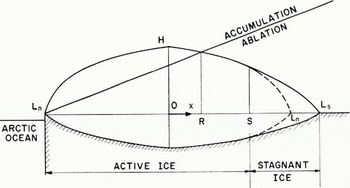
Fig. 5. Idealized ice-age ice sheet which is shrinking. The position S separates stagnant from active ice
The location s in Figure 5 represents the point of separation of the stagnant ice from the active ice a horizontal distance S from the ice divide. Between x = 0 and x = S the profile of the upper surface of the southern half of the ice sheet is the mirror image of the profile of the northern half. This similarity in profiles follows from the requirement that the ice thickness at
In the stagnant region the rate of change of the ice surface is
This equation will hold for all values of x equal to or greater then S. The ice thickness (h + d) at x = S obtained from equation (20),(21) and (22) is
If this equation is substituted into equation (30) and S is held constant, the following expression is obtained for the rate of change of L n:
As expected, this rate of change approaches zero as L n, S, and L S approach the same value. In the region in which ice is active, 0 ⩽ x ⩽ S the fulfillment of the condition of conservation of mass requires that the following equation be valid:

If equations (20), (25) and (22) are substituted into the left-hand side of this equation, and S again is held constant, we find that
With the use of equation (32) this last equation reduces to
which can be reduced further to
Placing equation (35b) into equation (32) gives
If now equation (23) is solved for R in terms of L n and this solution is placed into equation (36), a differential equation in L n is obtained whose solution gives the time dependence of L n, in other words the solution of our problem.
The exact solution of equations (36) and (23) obviously will be a rather complicated expression relating L n with time. However, without developing the exact solution, it is possible to obtain from these equations reasonable estimates of the time required to reach a new equilibrium profile. We now consider two cases of shrinking ice sheets. In one case the shrinkage of the ice sheet is due primarily to a rise in the elevation of the snow line, that is, to an increase in s. In the other case, the shrinkage results from an increase in the ablation rate and a decrease in the accumulation rate.
Increased Elevation of the Snow Line
If for some reason the snow-line elevation is raised while the accumulation and ablation rate remain constant, the effect is to reduce the distance R shown in Figures 4 and 5. Suppose that the increase in snow-line elevation is large enough that the new equilibrium size of the ice sheet is appreciably smaller than the original. Under these conditions the term
whose solution is
where L e is the original half-width of the ice sheet. This equation is almost the same as equation (16), which gives the shrinkage time of an ice sheet containing no accumulation. (The chief difference between the two expressions for the time is that one contains the factor
Increased Ablation and Decreased Accumulation Rates
Suppose that the shrinkage of an ice sheet is induced, not by an increase in the snow-line elevation, but rather through a decrease in the accumulation rate and an increase in the ablation rate. If again we assume that the ablation rate is at least twice the accumulation rate, both before and after the change in rates, we can make use of the fact that R is approximately equal to L. A better approximation for R, found by letting R = L in the right-hand side of equation (23), is
and
The substitution of equation (39b) into equation (36) gives
which can be rewritten as
where L e is the new equilibrium half-width and is given by
The solution of equation (41) is

where
and
We are interested in the situation in which the old equilibrium width L e is much greater than the new width L e. When

For t < t 0 this equation becomes
From equation (44b) we find that the time required to reduce the old equilibrium half-width L e by a factor
Through the use of equations (26) and (43) this equation reduces to

where a* and ā * are the original values of the accumulation and ablation rates.
The shrinkage time given by equation (45b) is considerably longer than that given by equation (16). For example, if
Summary
The results of the analysis presented in this paper can be summarized as follows. The time required to build up an ice-age ice sheet is of the order of 15,000 to 30,000 yr. if the accumulation rate over the ice sheet is in the range of 0.2 to 0.6 m./yr. Although there is no way known of obtaining paleo-accumulation rates, it can be argued that these rates are reasonable, in light of what is known about accumulation on the Greenland Ice Sheet. A period of time of the range of 15,000 to 30,000 yr. is of the order of the duration of an ice age or a substage of an ice age. The possibility arises, therefore, that the build-up of an ice sheet indeed may trigger off the mechanism which causes the ultimate destruction or temporary recession of the ice sheet. If such is the case, this result would favor an ice-age theory, such as that proposed by Ewing and Donn, which depends on a triggering action.
It has been shown in this paper that the time required for the disappearance of an ice-age ice sheet is smaller than the build-up time provided that the average ablation rate is at least twice the average accumulation rate and that ablation occurs over an appreciable area during shrinkage. The rapid disappearance of the last ice-age ice sheets can be understood on the basis of these results.
All the calculations were carried out on the basis of the theory of perfect plasticity. Clearly it would be desirable to repeat these calculations using Glen’s creep law. Such a calculation probably would yield valuable information on possible pulsations in the dimensions of an ice sheet, both during its growth and its retreat. We doubt that the refined calculation would lead to an appreciable alteration in the build-up and shrinkage times found in this paper. Since paleo-accumulation and ablation rates are not known, any small differences between the results of a refined calculation and the rough analysis of the present paper would be of little significance.


