


Introduction
Ice cores are valuable archives of paleoclimate information. Reconstruction of atmospheric composition with respect to gases, elements, and particles and also with respect to transport mechanisms during distinct climate periods are central foci of ice core research (Dansgaard and others, Reference Dansgaard1993; Mahowald and others, Reference Mahowald1999; Petit and others, Reference Petit1999; Johnsen and others, Reference Johnsen2001; Lüthi and others, Reference Lüthi2008). The detection of microorganisms and other biological material in ice cores across climate periods (Priscu and others, Reference Priscu1998; Christner and others, Reference Christner2000; Abyzov and others, Reference Abyzov2001; Christner and others, Reference Christner, Mosley-Thompson, Thompson and Reeve2003; Priscu and Christner, Reference Priscu, Christner and Bull2004) has opened new avenues for the analyses of organic matter (OM) in ice cores at high temporal resolution (D'Andrilli and others, Reference D'Andrilli, Foreman, Sigl, Priscu and McConnell2017a; King and others, Reference King2019). These works have advanced our understanding of ice sheets in three important ways: (i) they are preserved records of diverse OM components, (ii) OM data integrates well with other geochemical and biological ice core data, and (iii) OM composition can be used to reconstruct atmospheric composition within and across climate periods. Therefore, OM composition, though the newest addition to paleoclimate ice core research, holds great potential to advance our understanding of Earth's carbon (C) cycling patterns across ancient and modern scales.
Ice sheets across the world are beginning to be recognized as important reservoirs in global C budgets (Hood and others, Reference Hood, Battin, Fellman, O'Neel and Spencer2015; Wadham and others, Reference Wadham2019), with both OM characterization at the bulk and molecular level at the forefront of the exploration of pivotal ecological changes of our past and impact in the future (e.g. Grannas and others, Reference Grannas, Hockaday, Hatcher, Thompson and Mosley-Thompson2006; Bhatia and others, Reference Bhatia, Das, Longnecker, Charette and Kujawinski2010; D'Andrilli and others, Reference D'Andrilli, Foreman, Sigl, Priscu and McConnell2017a; Brogi and others, Reference Brogi2018). However, incorporating OM analyses in paleoclimate ice core research at high temporal resolution is still in its infancy and few datasets exist that combine ongoing geochemical measurements with quantitative and qualitative OM characterization at high temporal resolution (D'Andrilli and others, Reference D'Andrilli, Foreman, Sigl, Priscu and McConnell2017a; King and others, Reference King2019). The first report presented diverse OM fluorescence signatures of ancient and modern Antarctic ice cores driven by paleoclimate trends of past C production in the Southern Hemisphere (D'Andrilli and others, Reference D'Andrilli, Foreman, Sigl, Priscu and McConnell2017a). In that work, OM markers were identified unique to the last glacial maximum (LGM), deglaciation, and the early to mid-Holocene, which set the foundation for further Antarctic fluorescence OM investigations from new and archived ice cores (D'Andrilli and others, Reference D'Andrilli, Smith, Dieser and Foreman2017b). Together, both studies reported distinct OM composition unique to each climate period, though only related to regional influences of the Southern Hemisphere. If we are to truly realize the potential of OM characterizations in surface-to-deep ice core research in both hemispheres, we need to begin with descriptions from Northern Hemisphere ice cores, compare across datasets, and eventually expand OM research to include ice cores that cover vast spatiotemporal scales of other polar and alpine environments.
Continuous (surface-to-deep) ice core records are required for detailed paleoclimate research. As ice core research is highly collaborative, continuous measurements are restricted to small sample volumes to maintain high temporal resolution; therefore, characterizing ice core OM requires doing a lot with little volumes. Fluorescence spectroscopy is a bulk optical technique that offers a way to measure chromophoric (absorbing) and fluorophoric (fluorescing) OM pools rapidly, with minimal sample volumes required (~5 mL), maintaining the possibility to preserve relatively high temporal resolution necessary for ice core research. Fluorescence spectroscopy generates a wealth of information useful to characterize OM composition, origin and reactivity in the environment (Coble and others, Reference Coble, Green, Blough and Gagosian1990; Coble and others, Reference Coble, Del Castillo and Avril1998; Stedmon and others, Reference Stedmon, Markager and Bro2003). Thus far, this technique has shown promising results in paleoclimate research (D'Andrilli and others, Reference D'Andrilli, Foreman, Sigl, Priscu and McConnell2017a), and remains the most sensitive technique to discern diverse OM compositions with minimal sample volumes when employing continuous flow analysis systems.
Our objectives were to (i) chemically characterize OM fluorescence in Arctic ice cores at high temporal resolution, (ii) compare fluorescent OM composition within and across ice cores over space (regionally and globally) and time (ancient and modern scales), and (iii) reconstruct atmospheric OM compositions across ancient and modern scales with age and temperature data. We used Excitation Emission Matrices (EEMs) (Coble and others, Reference Coble, Green, Blough and Gagosian1990) and parallel factor (PARAFAC) analysis (Stedmon and Bro, Reference Stedmon and Bro2008; Murphy and others, Reference Murphy, Stedmon, Graeber and Bro2013) to identify OM compositions of Arctic ice cores and determine possible source origins. Trends of OM compositions, fluorescence intensities and relative concentrations within and across different climate periods are presented as a function of temperature and compared with an established record from Antarctica. Quantitative comparisons of each OM composition type were used to identify similar chemical species in both hemispheres. We used these data to infer modern and ancient paleoclimate fluorescent OM markers useful for future atmospheric reconstructions and potentially for other ice-sheet and/or low-C environmental studies. Here, we present ancient and modern Arctic ice core OM fluorescent composition and temperature records from the Arctic Circle Traverse 2010 (ACT-10), the Greenland Ice Sheet Project 2 (GISP2) of Greenland, and the Agassiz Ice Cap (hereafter, Agassiz) of Canada, and their comparisons with ice core OM from the West Antarctic Ice Sheet Divide (WD, Antarctica), advancing our understandings of OM records from ice sheets on a global scale and propelling collaborative OM characterization research in the paleoclimate community.
Methods
Sample locations
The three Arctic ice coring sites were in Greenland and Canada (Fig. 1; ACT-10, GISP2 and Agassiz). Ice core locations, collection dates, range of depths, ages and temporal scales are provided in Table 1. Modern ACT-10 ice was collected in 2010 from three spatially separated basins and descriptions of the ice cores, elevations, spatial distances from the coast and annual accumulation rates were reported in Miège and others (Reference Miège2013). GISP2 ice cores were collected in 1988 and archived at the National Science Foundation Ice Core Facility (NSF-ICF). Though the full core spanned depths to 3258 m, only 23 m were melted in 2012 for this work, capturing the end of the LGM in the Northern Hemisphere. The ice accumulation rate at GISP2 (Meese and others, Reference Meese1997; Stuiver and Grootes, Reference Stuiver and Grootes2017) was comparable to that of WD (WAIS Divide Project Members, 2013). Agassiz ice cores were collected in 2011 from the Agassiz Ice Cap, Ellesmere Island, Nunavut Territory, Canada, and a portion of the modern ice (2.72–15.63 m) was melted for this work. Detailed records of surface temperatures, seasonal changes and precipitation trends were previously reported (Fisher and others, Reference Fisher, Koerner and Reeh2016; Lecavalier and others, Reference Lecavalier2017). WD data are included for an Antarctic OM comparison to the Northern Hemisphere ice core records presented here. Detailed records of its environment and OM characterization were previously reported (WAIS Divide Project Members, 2013; D'Andrilli and others, Reference D'Andrilli, Foreman, Sigl, Priscu and McConnell2017a).

Fig. 1. Ice core sites in Canada and Greenland, showing the Agassiz Ice Cap (Agassiz), the Greenland Ice Sheet Project 2 (GISP2) and the Arctic Circle Traverse 2010 (ACT-10). The ACT-10 basins are labeled A, B and C, and represent the traverse route (70 km) starting at A and ending at C. Figure generated with QGIS software.
Table 1. Ice core location descriptions, collection years, depths from the surface (meters; m), ages (year; yr, and kiloyears; kyr), categorical temporal scales and fluorescence data organization of Excitation Emission Matrices (EEMs) sample numbers, parallel factor (PARAFAC) analysis model names and sample numbers used in PARAFAC analysis

a Dating scale from Miège and others (Reference Miège2013).
b Dating scale from Meese and others (Reference Meese1997).
c Dating scale from Fisher and others (Reference Fisher, Koerner and Reeh1995) and Lecavalier and others (Reference Lecavalier2017).
d Dating scale from WAIS Divide Project Members (2013).
e Organic matter data reported in D'Andrilli and others (Reference D'Andrilli, Foreman, Sigl, Priscu and McConnell2017a).
f Supplementary PARAFAC model using WD data collected not reported in D'Andrilli and others (Reference D'Andrilli, Foreman, Sigl, Priscu and McConnell2017a).
PARAFAC sample numbers refer to the number of EEMs used for each model.
Ice core collection, preparation and melting
Ice cores (ACT-10 and GISP2) were collected and transported to the NSF-ICF in Denver, Colorado, USA, for core processing. ACT-10 and GISP2 cores were cut into 3 × 3 × 100 cm sections and transferred to the Desert Research Institute in Reno, Nevada, USA, for continuous melting (4.5 mL min−1) in a closed continuous flow analysis (CFA) melting system (McConnell and others, Reference McConnell, Lamorey, Lamber and Taylor2002; McConnell and others, Reference McConnell, Aristarain, Banta, Edwards and Simoes2007; McConnell and others, Reference McConnell2014). Agassiz ice cores were processed at the Geological Survey of Canada, shipped to the Desert Research Institute, and cut into 3 × 3 × 100 cm sections just prior to melting. Ice core samples containing visible cracks or fractures were removed prior to melting and discarded from further analyses. Deionized water blanks were routinely run through the CFA melting system (every 6 m of ice core) to minimize contamination and monitor instrument performance.
Discrete samples for OM analyses by EEMs were collected using a sample collector (Model 223; Gilson). Meltwater from the CFA system was directed to the sample collector and dispensed into combusted amber glass vials with septa lids, maintained at 4 °C. A detailed description of CFA melting settings, discrete meltwater collection for OM analyses and system maintenance was previously reported (WAIS Divide Project Members, 2013; D'Andrilli and others, Reference D'Andrilli, Foreman, Sigl, Priscu and McConnell2017a). Samples were not filtered to avoid filter contamination. Amber glass vial lids were tightened after meltwater allotment (each vial filled to ~5 mL) and samples were stored in the dark at 4 °C prior to shipment and analysis. ACT-10, GISP2 and Agassiz ice cores were essential components to the WD project for preparation, method optimization and data interpretation and were melted either just before or at the conclusion of the WD project (2010–2012). Water isotopes (δ 18O [‰]) were collected for GISP2 and Agassiz ice following reported protocols outlined for WD in Marcott and others (Reference Marcott2014) as a proxy for air temperature. To evaluate changes in air temperatures for ACT-10 ice cores, we used available data through the NOAA-ESRL Physical Sciences Laboratory, Boulder, Colorado, USA, from their website (https://www.esrl.noaa.gov/). Temperature data were normalized to the 1981–2010 average (Model NCEP/NCAR Reanalysis 1; Kalnay and others, Reference Kalnay1996; Kistler and others, Reference Kistler2001) using the 2 m air temperature boundaries as follows: 65.7125–88.542 latitude and 290.625–320.625 longitude.
Ice core OM absorbance and fluorescence spectroscopy
All samples were measured for absorbance at a single excitation wavelength (254 nm) and then scanned from 190 to 1100 nm using a Genesys 10 Series (Thermo-Scientific, Massachusetts, USA) Spectrophotometer with a 1 cm pathlength microvolume (70 μL) cuvette and VISIONlite software. This was a necessary step prior to the fluorescence spectroscopy measurements. All samples had measured absorbance values at 254 nm below the daily Milli-Q water blank, and so no sample dilution was required prior to fluorescence spectroscopy measurements at the same pathlength. Therefore, all OM absorbance characteristics from each ice core were inferred from the excitation spectra of the fluorescence measurements. For further investigation of optically active OM absorbance properties, future studies may benefit from longer pathlength cuvettes when larger sample volumes are available. A detailed description of the absorbance method and its importance prior to fluorescence measurements is provided in D'Andrilli and others (Reference D'Andrilli, Foreman, Sigl, Priscu and McConnell2017a) and referenced within.
EEMs were generated by a Horiba Jobin Yvon Fluoromax-4 Spectrofluorometer equipped with a Xenon lamp light source and a 1 cm pathlength quartz cuvette. Excitation wavelengths were scanned from 240 to 450 nm in 10 nm (GISP2 and Agassiz) and 5 and 10 nm (ACT-10) wavelength intervals, and emission wavelengths were recorded between 300 and 560 nm in 2 nm increments. We used ACT-10 to optimize excitation wavelength data acquisition across 5 and 10 nm increments, prior to GISP2 and Agassiz data collection. Data integration time was 0.25 s and data acquisition was carried out in signal/reference mode using a 5 nm bandpass on both excitation and emission monochromators, normalizing the fluorescence emission signal with the excitation light intensity. Fluorescence output was normalized to the area under the Raman peak of a Milli-Q water sample each day at excitation: 350 nm and emission: 365–450 nm. EEMs were blank corrected with Milli-Q water placed in a combusted amber glass vial with a pierced septa lid and shaken for 2 min at 4 °C. Post processing of the fluorescence data was completed in MATLAB to generate corrected EEMs which included sample corrections for Raman scattering and the method blank subtraction. Milli-Q water samples were scanned each day of experimentation to monitor instrument performance and cuvette contamination. Total EEMs sample numbers for each ice core site are provided in Table 1.
PARAFAC analysis
EEMs are commonly modeled with PARAFAC analysis to identify specific fluorescence regions that characterize the variation in OM composition from aquatic and terrestrial environments (Stedmon and Bro, Reference Stedmon and Bro2008; Murphy and others, Reference Murphy, Stedmon, Graeber and Bro2013). Put simply, PARAFAC analysis models the EEMs data by decomposing the overlapping fluorescence signatures in each EEM into individual regions of fluorescence (identified components). This assists with OM chemical characterizations as the modeled components are easy to visualize, outliers are identified, and trends can be tracked across datasets more conveniently. Individual PARAFAC models were generated by Decomposition Routines for Excitation Emission Matrices (drEEM) (Murphy and others, Reference Murphy, Stedmon, Graeber and Bro2013) and the N-way toolbox (Stedmon and Bro, Reference Stedmon and Bro2008) scripts in MATLAB to identify fluorescent OM markers for each ice core and comparisons across ice core sites (Table 1). The ACT-10 PARAFAC model included data collected at excitation wavelength increments of 10 nm. Non-negativity constraints were applied, and the models were validated by split half analysis having a Tucker correlation coefficient (TCC) > 0.95, and subsequently re-validated using the least-squares model in the final output (Murphy and others, Reference Murphy, Stedmon, Graeber and Bro2013). The modeled results list components in numerical order according to highly variable and dominant signatures in the EEMs dataset such that C1 > C2 > C3 > … > Cn. In general, the component labels do not indicate a characteristic OM type, rather it is an arbitrary label used to delineate one fluorescence region from another. The results were then used to characterize OM composition as a record of past and recent C sources transported to polar regions.
In the event that PARAFAC only produces one component, the component, ‘C1’, then represents the complete fluorescence description of the EEMs dataset analyzed. We acknowledge that this may arise from a lack of statistical power due to smaller sample sizes and/or from a lack of variation in OM composition in the dataset. Additionally, a supplemental WD PARAFAC model (a subset of the larger WD dataset from D'Andrilli and others (Reference D'Andrilli, Foreman, Sigl, Priscu and McConnell2017a); WDsupp, Table 1) was generated to directly compare OM trends with the Northern Hemisphere GISP2 ice core record of the same dates (~19.0–17.0 kyr BP 1950; radiocarbon years [hereafter BP]). WD data were available from D'Andrilli and others (Reference D'Andrilli, Foreman, Sigl, Priscu and McConnell2017a), but not published in that work. Individual PARAFAC component fluorescence intensities for ACT-10, GISP2, Agassiz and WD ice cores were calculated by drEEM and reported in Raman Units (R.U.).
OM fluorescence characterization
Fluorescing OM peaks from the ACT-10, GISP2 and Agassiz PARAFAC models were characterized by the commonly labeled fluorophore regions and descriptions (Table 2; Coble and others, Reference Coble, Green, Blough and Gagosian1990; Coble and others, Reference Coble, Del Castillo and Avril1998) and with peaks from laboratory chemicals, freshly collected ecosystem samples, and more processed and commercially available environmental samples (Fig. S1). EEMs of laboratory chemicals included phenylalanine, tyrosine, tryptophan and vanillic acid, representing simpler, less aromatic organic acids. The chemical structures of those chemicals are also provided in Figure S1 for reference. EEMs of International Humic Substances Society (IHSS) fulvic acids represented different terrestrial and microbial end-members (Suwannee River [Georgia, USA] and Pony Lake [Antarctica]). EEMs of freshly collected environmental samples represented unprocessed, natural, and complex organic materials compared to laboratory standards, including semi-arid Montana soils and the upper reach of the Yellowstone River, western Montana, USA (Fig. S1).
Table 2. EEMs fluorescence descriptions of aquatic organic matter markers, potential sources, reactive nature types and possible fluorescence chemical species overlapping with commonly used peak regions

Arctic and Antarctic OM fluorescence comparison calculations
All models were quantitatively compared to reveal similar OM signatures and therefore chemical species over space and time. Comparing separate models was specifically chosen to reduce sample biases when using a single PARAFAC model approach (D'Andrilli and others, Reference D'Andrilli, Foreman, Sigl, Priscu and McConnell2017a, Mostofa and others, Reference Mostofa, Jie, Sakugawa and Liu2019) and allows for quantitative comparisons using Tucker's correlation calculations. Significant PARAFAC model component comparisons were determined from three calculations: (1) joint excitation and emission loading shift- and shape-sensitive congruence coefficients (SSC) (Wünsch and others, Reference Wünsch, Bro, Stedmon, Wenig and Murphy2019), (2) TCC calculated on excitation loadings (Tucker, Reference Tucker1951; Lorenzo-Seva and ten Berge, Reference Lorenzo-Seva and ten Berge2006), and (3) SSC calculated on emission loadings (Wünsch and others, Reference Wünsch, Bro, Stedmon, Wenig and Murphy2019). The SSC is a modified calculation of Tucker's for data obtained by fluorescence spectroscopy (Wünsch and others, Reference Wünsch, Bro, Stedmon, Wenig and Murphy2019). Three separate calculations were used to statistically compare the PARAFAC components' chromophoric (light-absorbing), fluorescing (light-emitting) and combined optically active OM fractions. Loading scores were modeled during PARAFAC analysis and normalized to 1. For detailed descriptions of TCC and extensions to the SSC calculations for EEMs and PARAFAC data, see Wünsch and others (Reference Wünsch, Bro, Stedmon, Wenig and Murphy2019). The minimum requirement for significantly similar fluorescent OM components from one or more PARAFAC models is TCC and SSC ⩾0.9. TCC and SSC > 0.95 describes nearly identical fluorescent chemical species from components of different models. The hierarchical clustering of PARAFAC component excitation and emission spectra loadings was conducted using the complete linkage method. Dendrograms visually expressed this clustering. Clustering and dendrograms were constructed using the ‘heatmap.2()’ function within the ‘gplots’ package in R version 3.6.3 (R Core Team, 2020).
Results and discussion
PARAFAC model results and organization for OM characterization
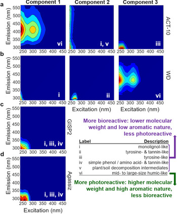
Results of the individual PARAFAC models explained 96.5% (ACT-10), 96.6% (WD), 92.0% (GISP2) and 95.0% (Agassiz) of the EEMs variation per dataset, respectively. Organizing the four models in a table format (Fig. 2), structured by individual models as rows and component order as columns, created a simple visual mechanism for initial comparison among different OM signatures and models. Here, the component listing labels correspond to the dataset variability of each model, i.e. the higher the number of components, the more variation in the data. We used this organized scheme to show different types of OM listed sequentially, a metric of OM dominance in each core. The PARAFAC analysis results showed similar OM fluorescence signatures (C1, C2 and C3; Fig. 2) to each other and a variety of OM across aquatic and terrestrial environments (Fig. S1), describing diverse OM compositions from simple to complex chemical species. The four models differed in total component number (1 versus 3) and ordering sequence of OM type, describing varying dominant chemical species likely related to their spatial influences over time (Table 1). Based on the EEMs data (examples in Fig. S2), two-component PARAFAC models were also attempted for the GISP2 and Agassiz datasets; however, no successful validation was achieved within acceptable statistical conditions. The WD PARAFAC model results, reproduced in Figure 2b, represented the Southern Hemisphere OM record spanning three different climate periods used for comparison (D'Andrilli and others, Reference D'Andrilli, Foreman, Sigl, Priscu and McConnell2017a). Figure 2 summarizes naturally occurring OM fluorescence descriptions and characterizations from Table 2 (Coble and others, Reference Coble, Green, Blough and Gagosian1990; Coble and others, Reference Coble, Del Castillo and Avril1998; Stedmon and others, Reference Stedmon, Markager and Bro2003; Coble and others, Reference Coble, Lead, Baker, Reynolds and Spencer2014) to visually compare each PARAFAC component's OM signature and description within a model and among models.

Fig. 2. A global perspective of ice core organic matter fluorescence (components one, two and three [C1, C2 and C3]) identified by individual multivariate parallel factor (PARAFAC) analysis models for ice cores: (a) Arctic Circle Traverse 2010 (ACT-10), (b) West Antarctic Ice Sheet Divide (WD) (reproduced from D'Andrilli and others (Reference D'Andrilli, Foreman, Sigl, Priscu and McConnell2017a)), (c) Greenland Ice Sheet Project 2 (GISP2) and (d) Agassiz Ice Cap. Fluorescence data were reported in Raman Units. Each PARAFAC component is accompanied by chemical description labels (i–vi), with summarized definitions of OM type and reactive nature in the legend.
Since naturally occurring OM is a ‘supermixture’ of diverse heterogeneous species, it may be uncommon to generate one PARAFAC component from a dataset. Such a result suggests one viable outcome of one fluorescence region, describing a lack of qualitative variability in OM type (Murphy and others, Reference Murphy, Stedmon, Graeber and Bro2013); however, recent evidence suggests it is more frequent than we tend to expect across diverse OM ecosystems (Wünsch and others, Reference Wünsch, Bro, Stedmon, Wenig and Murphy2019). Therefore, the use of individual PARAFAC models and their results created a mechanism for direct comparisons across models, regardless of the number of components. Individual model comparisons target different research questions than a joint model can answer, without confounding biases arising from different datasets (D'Andrilli and others, Reference D'Andrilli, Foreman, Sigl, Priscu and McConnell2017a, Mostofa and others, Reference Mostofa, Jie, Sakugawa and Liu2019). The WD OM record showed examples of the strength of both approaches, specifically targeting different research questions to decipher ice core OM and its contribution in paleoclimatology (D'Andrilli and others, Reference D'Andrilli, Foreman, Sigl, Priscu and McConnell2017a). Here, we highlight the strength of individual modeling efforts and target what types of OM are in ice cores from different regions over vastly different temporal scales to contribute a new approach to ecosystem understanding from C cycling events of our past. Importantly, our descriptions of OM character are provided as a record of the past and recent atmospheric composition, treating OM the same way as other materials that are deposited and preserved in ice. Where applicable, trends potentially related to atmosphere exposure in the firn ice prior to preservation are reported and discussed.
Arctic modern OM fluorescence characterization: Greenland ACT-10
ACT-10 ice cores contained three fluorescence components (Fig. 2a). These cores represented a record of late Holocene C deposited from the recent past. ACT-10 contained a dominant ‘humic-like’ component (C1; Fig. 2a), a signature associated with complex OM production and degradation found worldwide, but most prevalent in terrestrial forested and wetland environments (peak A; Table 2) (Coble and others, Reference Coble, Green, Blough and Gagosian1990; Coble and others, Reference Coble, Del Castillo and Avril1998; Parlanti and others, Reference Parlanti, Wörz, Geoffroy and Lamotte2000), potentially representing C produced from surrounding continents and transported via Northern Hemisphere and Arctic air circulation patterns. Within the ‘humic-like’ category, there exists a gradient of OM that is commonly characterized by the peak A label. To further describe this material, we evaluated this signature with our catalog of diverse OM from terrestrial environments (Fig. S1). This signature shares similarities with naturally collected OM of semi-arid soils (Romero and others, Reference Romero2017) and the Yellowstone River (Fig. S1 bottom panel), environments that receive allochthonous inputs from higher plants/soils and are highly impacted by microbes. Notably, this signature was considerably different than Suwannee River fulvic acid OM (Fig. S1) where the peak maximum for Suwannee River exists at higher emission wavelengths. It also shared more commonalities with microbially produced Pony Lake fulvic acid OM (Fig. S1), suggesting that it may reflect terrestrial OM of plant/soil origin as well as the biodegraded products of that complex material. OM fluorescence signatures at higher emission wavelengths (>350 nm) are generally linked to larger, more aromatic and complex chemical species susceptible to photooxidation when exposed to sunlight. Therefore, these data provided strong evidence of complex OM of terrestrial influence, transported to southeast Greenland from environments rich with plants, soils and microbes.
ACT-10 C2 contained OM fluorescence at low excitation and broad emission wavelengths (250/300–560 nm), representing a mixture of simple and more complex OM. Its presence in ACT-10 may describe effective Aeolian transport of diverse biodegraded OM chemical species also found in terrestrial soils (Zhao and others, Reference Zhao, Zhang and He2012; Romero and others, Reference Romero2017; Romero and others, Reference Romero, Engel, D'Andrilli, Miller and Wallander2019). This component represents fluorescence from multiple OM types in ACT-10 due to the common fluorescence across multiple samples at low excitation wavelengths (240–260 nm) (Fig. S2a). Since this signature does not yet have a commonly used corresponding peak label, we characterized the OM by splitting the fluorescence into two sections and comparing them with other ice core and environmental fluorescence data from the literature. We used the monolignol-like OM characterization for WD C1 reported in D'Andrilli and others (Reference D'Andrilli, Foreman, Sigl, Priscu and McConnell2017a), reproduced in Figure 2b, to characterize the low emission (300–320 nm) wavelength region of ACT-10 C2. This fluorescence region is characteristic of simple phenolic chemical species known to be ubiquitously found in the environment that are characteristically different from tyrosine-like (peak B) fluorescence (Aiken, Reference Aiken, Baker, Reynolds, Lead, Coble and Spencer2014) (Table 2, Fig. S1). The longer emission fluorescence signature (>350 nm) was characteristic of Northern Hemisphere soils undergoing decomposition with various land management schemes (Zhao and others, Reference Zhao, Zhang and He2012; Romero and others, Reference Romero2017; Romero and others, Reference Romero, Engel, D'Andrilli, Miller and Wallander2019) providing more evidence beyond ACT-10 C1 of transported terrestrial OM to southeastern Greenland. Ice-sheet environments without surface meltwater pools, ponds and/or lakes that lack higher plant vegetation can only have these types of signatures as a result of Aeolian transport of C produced in external environments, supporting the use of OM signatures in ice cores as a record of regional and global C over time.
ACT-10 C3 was characteristic of tyrosine-like OM (peak B; Table 2) and also with phenylalanine and tyrosine fluorescence (Fig. S1). This signature represents microbially altered OM (Coble and others, Reference Coble, Green, Blough and Gagosian1990; Coble and others, Reference Coble, Del Castillo and Avril1998) with low aromatic nature, the chemical species of which are commonly favored in biological processing mechanisms (Parlanti and others, Reference Parlanti, Wörz, Geoffroy and Lamotte2000). OM character defined as ‘amino acid-like’ (peaks B and T; Table 2) is linked with microbial processes in aquatic and terrestrial environments (a review of diverse examples in Coble and others, Reference Coble, Lead, Baker, Reynolds and Spencer2014). Of the two amino acid-like OM fluorescence peak labels, B refers to more degraded microbial products or other peptide material and is less commonly associated with freshly produced material. Therefore, its presence may indicate heterotrophic microbial degradation pathways, though delineating degradation of terrestrial versus marine origin was not possible with these data. We acknowledge the potential influence of marine OM from local wind patterns to the southeastern region of Greenland (Proshutinsky and others, Reference Proshutinsky, Dukhovskoy, Timmermans, Krishfield and Bamber2015); however, we were not able to confirm a more marine-like OM signature (peak M; Table 2) within this dataset. The lack of tryptophan-like OM fluorescence (peak T; Table 2, Fig. S1) suggests ACT-10 did not contain freshly produced OM, which may indicate low contributions from in situ autotrophic processes after deposition.
Arctic ancient and modern OM characterization: Greenland GISP2 and Canadian Agassiz
GISP2 and Agassiz PARAFAC models produced one component each with similar fluorescence. These components (Figs 2c, d) shared fluorescence regions with multiple types of chemical species such as monolignol-, tannin- and amino acid-like (phenylalanine and tyrosine) OM, describing two major classes of OM found in the environment over different climate periods, simple phenolic lignin precursors or degraded products, e.g. vanillic acid (Fig. S1) and amino acids. Our Agassiz OM character results that suggested amino acid-influenced OM (similar to peak B; Table 2) were consistent with another report from Ellesmere Island on John Evans Glacier that also detected amino acids and other small molecular weight compounds by EEMs and 1H nuclear magnetic resonance spectroscopy (Pautler and others, Reference Pautler2012). Two fluorescence maxima are observed for Agassiz C1, compared to GISP2. These differences suggest varying contributions of characteristically-distinct OM in each ice core on different temporal scales – higher contributions from simple phenolic, amino acid- and tannin-like chemical species in Agassiz and lower contributions from tannin-like chemical species in GISP2.
It is likely that the amino acid-like OM of each ice core was influenced by microbial communities shaped by location and climate. Pautler and others (Reference Pautler2012) speculated that microbial variation of the Canadian Arctic was not only a function of atmospheric deposition but the differential incorporation of microbes into the ice of its environment, though variation may be more apparent in the surface or basal ice under different thermal regimes (Dubnick and others, Reference Dubnick, Sharp, Danielson, Saidi-Mehrabad and Barker2020). Even within the late Holocene, regional wind patterns across the Arctic Ocean show different sources reaching Ellesmere Island than eastern Greenland (near ACT-10) and it is possible that the location of Agassiz is most locally influenced by coastal winds of Baffin Bay (Proshutinsky and others, Reference Proshutinsky, Dukhovskoy, Timmermans, Krishfield and Bamber2015). Thus, these OM fluorescence variations can be influenced by multiple regional and local environmental factors including coastal proximity, regional air circulation, local wind patterns, and resident and transported microbial communities. Like ACT-10, the lack of resolved tryptophan-like OM signatures (peak T; Table 2) suggested minimal contributions of freshly produced OM by microbes, and further biological investigation would be required to identify the extent of microbial transformations following deposition.
Spatiotemporal comparisons of fluorescent OM character
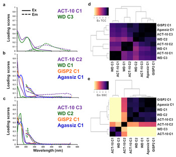
Similar OM fluorescence signatures and therefore chemical characterizations (OM type and potential source origin) were detected for these ice cores (Fig. 2, Fig. S1) suggesting similarities across regional and global spatiotemporal scales. To compare the PARAFAC components with similar fluorescence in more detail, we selected three groups to evaluate that had characteristically different signatures: Group 1, exclusive to OM type ‘vi’, Group 2, at least containing the type ‘i’, and Group 3, a mixture of OM containing types ‘ii’, ‘iii’, and ‘iv’ (Fig. 2). For these groups, the PARAFAC model spectral loadings for excitation and emission were superimposed to show their magnitudes and wavelength ranges (Figs 3a–c). In Figures 3a–c, the superimposed excitation and emission spectra represented comparisons of chromophoric and fluorophoric OM, respectively. Excitation spectra described absorbing chemical species (chromophoric OM) whereas emission spectra described fluorescing chemical species (fluorophoric OM). Additionally, pairwise clustering was used to confirm near-identical OM species across all ice core components (Figs 3d, e). In general, the data clustered separately for OM fluorescence at higher emission wavelengths from lower excitation and emission wavelengths (Figs 3d, e), and variations at low excitation and emission wavelengths were observed (Figs 3b, c). Fluorescence similarities were regional (Greenland and Canada) and global (Arctic to Antarctic) across ancient and modern scales. From these comparisons, we identified specific fluorescence features that can be used for future paleo- and modern climate assessments of OM.

Fig. 3. Comparisons of PARAFAC analysis component excitation and emission spectral loadings for ice core organic matter of (a) ACT-10 C1 and WD C3, (b) ACT-10 C2, WD C1, GISP2 C1 and Agassiz C1, and (c) ACT-10 C3, WD C2, GISP2 C1 and Agassiz C1. Components are listed as C1, C2 and C3. Quantitative comparisons were calculated based on the component (d) Tucker congruence coefficients (TCC) (Tucker, Reference Tucker1951; Lorenzo-Seva and ten Berge, Reference Lorenzo-Seva and ten Berge2006) for excitation loadings and (e) shift- and shape-sensitive congruence coefficients (SSC) (Wünsch and others, Reference Wünsch, Bro, Stedmon, Wenig and Murphy2019) for emission. The colorscale for (d–e) indicates the TCC and SSC values with a maximum value of 1. Cluster analyses of the PARAFAC components were calculated from the TCC and SSC results (Tables S2a, b).
Group 1: mid- to large-size humic-like OM of the Holocene
Fluorescence for ACT-10 C1 was more broadly distributed over emission wavelengths compared to WD C3 although the peak maxima were located at the same wavelength (418 nm). While comparisons between ACT-10 and WD OM were not possible on the same late Holocene timescale, these ‘humic-like’ signatures indicate strong evidence for more complex materials being produced in our modern past, that we identify as a unique Holocene OM marker. These two components were significantly similar (SSC = 0.95; Table S1) and clustered together, describing identical OM in both polar regions (Figs 3d, e). We note that ‘humic-like’ OM was more dominant in the ACT-10 record and speculate that the Greenland ice sheet receives more terrestrially derived OM due to its proximity to other continents compared to Antarctica. Therefore, this OM type and amount in the Arctic may be more indicative of Arctic air circulation patterns when forested, soil and wetland ecosystems are nearby. If any chemical composition differences of these two components (SSC = 0.05) exist, they were considered minor over large spatial (global) and temporal (ancient to modern) scales.
Group 2: monolignol-like OM and its linked fluorescence signatures across large spatiotemporal scales
This group contained OM having at least one fluorescence signature characteristic of monolignols (type ‘i’; Fig. 2) and we recognize that other fluorescing OM are present for ACT-10 C2, GISP2 and Agassiz within this group. We used the characterized WD C1 OM type from D'Andrilli and others (Reference D'Andrilli, Foreman, Sigl, Priscu and McConnell2017a) to establish this description of similar monolignol-like OM fluorescence in the Arctic ice cores. Monolignols are the small molecular compound precursors to larger lignin molecular chains of vascular plants and are ubiquitously found in the environment. Excitation spectra clustered more similarly than emission spectra across all ice cores. The excitation spectra for ACT-10 C2 and WD C1 were more significantly similar (TCC = 0.96) than when comparing ACT-10 C2 to GISP2 (TCC = 0.92) and Agassiz (TCC = 0.85) (Fig. 3d and Table S2a). Highly congruent excitation spectra (TCC > 0.95) that vary in loading scores represent a proxy of the relative quantity of the same OM chromophoric species among ice cores. These results indicate that Arctic ice cores contain very similar, but not identical monolignol-like chromophores regionally distributed over ancient and modern temporal scales. More identical monolignol-like chromophores, determined for ACT-10 and WD OM, describe global distribution across vast temporal scales. It is likely that they represent more bioreactive than photoreactive species in diverse environments, compared to larger lignin moieties, based on their chemical nature. However, further analysis of microbes using monolignols in heterotrophic degradation processes would be needed to confirm its bioreactivity in the environment.
The similarities of fluorescing OM within this group existed only at the lowest excitation and emission wavelengths (250/300 nm), but only comparisons between WD C1 and GISP2 C1, and WD C1 and Agassiz C1 produced emission correlations of SSC > 0.9 (Fig. 3e and Table S2b). Furthermore, at the same temporal scale, the comparisons between WDsupp data (characteristic of group 2; a subset of the WD data, Figs S3a–c) and GISP2 C1 yielded SSC = 0.95, describing nearly identical OM chemical character of the same climate period in opposite polar regions. This suggests abundant monolignol-like OM was produced in both hemispheres and circulated throughout Aeolian global conveyor belts. Most likely, the weak correlation of all the ice core comparisons for this group was due to the longer emission feature for ACT-10 C2 (i.e. the fluorescence ‘tail’). In our data, this feature was a unique Greenland Holocene signature and may represent a marker for microbial decomposition occurring in soils before being transported to southeastern Greenland.
Across both excitation and emission loadings, no pairwise component coefficients were greater than the 0.9 threshold for this group (Table S1), indicating no determination of identical species across the group's features. However, the variability of this group having monolignol-like character and other OM fluorescence distinguishes it as a separate marker. From the original WD ice core, monolignol-like fluorescence was detected in all climate periods (D'Andrilli and others, Reference D'Andrilli, Foreman, Sigl, Priscu and McConnell2017a) and the non-monolignol characteristic fluorescence, across varying wavelengths, was influenced by ecological changes of deglaciation and the Holocene. Therefore, this group may be characteristic of large and small ecological changes of our past (e.g. transition periods after the LGM, warming and cooling periods within the Holocene).
Group 3: amino acid- and tannin-like OM across large spatiotemporal scales
This group contained fluorescence at low excitation and emission wavelengths that were different from the monolignol-like category (group 2). Here, fluorescence of types ‘ii’, ‘iii’, and ‘iv’ (Fig. 2) are discussed without the inclusion of monolignols, though other simple phenolic compounds may fluoresce in this region (e.g. vanillic acid). Group 3 therefore spans the phenylalanine-, tyrosine- and tannin-like characterized OM fluorescence signatures (Fig. S1). Since group 3 was not characterized by resolved tryptophan-like OM fluorescence, it therefore represents an OM marker involving, but not exclusive to, microbial degradation of simple OM, as evident by the resolved tyrosine-like signature of ACT-10 C3 and the similar signatures for WD C2, GISP2 C1 and Agassiz C1. Additionally, this marker is easily discernable from the fluorescence ‘tail’ feature of ACT-10 C2, the proposed marker for microbial decomposition of simple and complex OM in soils.
The spectral loadings clustered most similarly (TCC and SSC > 0.90) across all ice cores for ACT-10 C3, WD C2, GISP2 C1 and Agassiz C1 (Figs 3c–e, Tables S1 and S2a, b) describing nearly identical bioreactive chemical species were globally distributed across ancient and modern scales. Analysis of components in Figure 3c showed more closely related OM of this type in the Arctic compared to Antarctic OM (Table S1). When specifically comparing Arctic Greenland and Canada data across the same temporal scale, Agassiz lacked more complex OM fluorescence, compared to ACT-10. These differences may be driven by local and regional influences; regional influences may extend to different OM sources and air circulation patterns and local influences may include coastal proximity, coastal winds, surface snow processes, OM/microbial consortia and ice preservation conditions. However, these are just suggestions based on the OM fluorescence differences from these data and more extensive OM and geochemical surveys of Holocene Arctic ice (either newly cored or from available ice storage repositories) would be needed to confirm such detailed information. From our data, when comparing across spatial and temporal scales, and despite similarities in both polar regions, this fluorescence technique can be used to target points for future inquiry.
Implications for Arctic and Antarctic OM concentrations from fluorescence data
All ice core data, when coupled with historical climate period data (end of the LGM, warming and cooling periods of the Holocene), revealed time-specific changes in OM quality. Such changes over time may also have characteristic changes in C quantity. While organic C concentrations were not available for this work, we used fluorescence intensity trends to discern relative increases and decreases in concentrations within the individual PARAFAC components (Murphy and others, Reference Murphy, Stedmon, Graeber and Bro2013). In the following sections, we compare the individual components and their intensities among ice cores based on their similar fluorescent OM composition (e.g. ACT-10 and WD, and GISP2 and Agassiz) rather than based on their spatial or temporal contexts. Where applicable, intensity signals that may relate to in situ OM transformations in the firn prior to preservation are discussed.
ACT-10 and WD
The ACT-10 basins differed in distance from the coastline, elevation and snow accumulation (Miège and others, Reference Miège2013), which have an influence on OM type and fluorescence intensities over space and time. To evaluate relative changes in C concentration from OM fluorescence trends over the longest time period, we present fluorescence intensities from basin C (Fig. 4a) having the lowest accumulation rates and being the farthest inland (Miège and others, Reference Miège2013) (Fig. 1). OM fluorescence intensities across ACT-10 basins A and B are provided in Figure S4, however basin-to-basin comparisons were beyond the scope of this work. Overall, ACT-10 C3 had the highest fluorescence intensities compared to C1 and C2, although those values (>0.01 R.U.) were characteristic of years 2000–2010 only. For C1 and C2, fluorescence intensities were variable over time, with an increase around 1996, describing increases in more humic- or lignin-like OM from plant and soil materials and their microbial breakdown products from Northern Hemisphere continents of the late Holocene. C3 fluorescence intensities showed a strong increasing trend over time, describing increases in tyrosine-like OM concentrations and larger contributions of microbially altered materials for the most recent years. It is likely that the last decade of data (2000–2010) describes an increase in microbial influences due to firn warming by increasing air temperature; notable increase in fluorescence intensities near the end of 1997. Before 1997, average fluorescence intensities were an order of magnitude lower, 0.00149 R.U., compared to 0.01041 R.U. after 1997. Therefore, we speculate that the fluorescence intensity trends may provide insight into surface decomposition processes occurring within the firn.

Fig. 4. Parallel factor component organic matter fluorescence intensities over time for ice cores: (a) Arctic Circle Traverse 2010 for basin C and (b) West Antarctic Ice Sheet Divide. Component labels are provided as C1, C2 and C3. For (a) time is provided as dated years of the late Holocene (Miège and others, Reference Miège2013) and for (b) time is provided in kiloyears (kyr) before present (BP) (WAIS Divide Project Members, 2013). Fluorescence intensities are reported in Raman Units (R.U.). The (*) symbol refers to the first observation of a resolved ‘humic-like’, plant/soil signature in the Holocene. LGM, Last Glacial Maximum; LD, last deglaciation.
Each climate period of WD contained fluctuating fluorescence intensities indicating varying concentrations of C1 and C2 (Fig. 4b; data generated from D'Andrilli and others (Reference D'Andrilli, Foreman, Sigl, Priscu and McConnell2017a) but not reported in that work). C3 fluctuations are shown across the 21.0 kyr record, however, the first observation of a resolved ‘humic-like’ signature of plant/soil origin was detected in the Holocene ~11.0 kyr BP (Fig. 4b). Overall, the largest fluorescence intensities were reported for C1 across all climate periods in the WD ice core and the Holocene contained the largest intensities of each OM type (C1, C2 and C3) comparatively. The Holocene was also characterized by having the lowest dust concentrations, lower sea-ice influence and the warmest temperatures (WAIS Divide Project Members, 2013), suggesting a potential correlation of OM concentration with temperature (D'Andrilli and others, Reference D'Andrilli, Foreman, Sigl, Priscu and McConnell2017a). Holocene photosynthetic productivity rates (Pg C a−1) were estimated to be more than double that of the LGM (Ciais and others, Reference Ciais2012), which linked increased biosphere C productivity to warmer temperatures. Using fluorescence intensities as a proxy for relative OM concentration changes, we explored these fluorescence intensity changes with relative temperatures further to infer how changes in past C productivity might be preserved in the ice core record.
GISP2 and Agassiz
GISP2 OM fluorescence intensities generally increased (more than doubled) from ~19.0 to 17.8 kyr BP, describing relative increases in OM concentrations from the transition of the LGM to Henrich Stadial 1 (Fig. 5a). This climate transition was marked with simultaneous changes in certain ecological responses associated with warming temperatures, such as sea-level rise and atmospheric methane concentrations (Mayewski and others, Reference Mayewski1997; Petit and others, Reference Petit1999; Clark and others, Reference Clark2009; Stuiver and Grootes, Reference Stuiver and Grootes2017). In that context, it is likely that those ecological changes also resulted in increased OM production from different sources (terrestrial, microbial, marine) with climate warming, as regional environments became more ice-free.

Fig. 5. Organic matter fluorescence intensities from PARAFAC analysis (component one; C1) and water isotope temperature records (δ 18O) for (a) Greenland Ice Sheet 2 Project (GISP2); isotope data smoothed over 100 point average, (b) Agassiz, and (c) the West Antarctic Ice Sheet (WD) subset supplemental (WDsupp) data. Insets for each panel show the relationship of C1 fluorescence intensity as a function of water isotopic value with correlation coefficients provided. The dashed line in (a) represents a weak association between variables. Error bars represent the range of years of each sample. Fluorescence intensities are provided in Raman Units (R.U.); kiloyears before present 1950 as kyr BP.
These paleoclimate implications were similar to that inferred from WD OM trends at the end of the LGM (D'Andrilli and others, Reference D'Andrilli, Foreman, Sigl, Priscu and McConnell2017a) with similar OM signals. GISP2 C1 contained different types of simple chemical species (Fig. 2c), however, without separately resolved fluorescence signatures, we can only report increases for it as a group of characteristically ‘simple’ OM concentrations, and not individual types. We use the term ‘simple’ to separate a category of low molecular weight and low aromatic molecular compounds from more complex, highly aromatic and larger compounds. Further molecular-level analysis and concentration measurements would be required to identify the different compositions and amounts linked to climate period changes since the LGM.
Fluctuations in Agassiz fluorescence intensities spanned an order of magnitude (0.0075–0.0136 R.U.) across a period of 60 years, and intensities from the oldest to youngest samples showed an initial increase after 1940, followed by a decrease (near 1980), and rebound by years 1990 and 2000. These temporal shifts could indicate changing OM concentrations of Agassiz's simple OM types despite this dataset having very few samples. Assuming these fluctuations are related to OM concentration over time for Agassiz, we explored temperature and other ecological variables that may drive such changes in the literature. Other reported Agassiz Ice Cap ice core data (e.g. temperature, elemental concentration and trapped gas) are commonly compared with Greenland ice cores on the same temporal scale because of their proximity and consistent findings (Koerner and others, Reference Koerner, Fisher and Goto-Azuma1999; Vinther and others, Reference Vinther2009; Lecavalier and others, Reference Lecavalier2017). Following that framework, it is possible that their general OM trends may also be similar, following similar regional influences.
Mean annual temperatures reported in the literature observed a cooling period in Greenland from 1950 to 1980 (Chylek and others, Reference Chylek, Dubey and Lesins2006), which was consistent with average temperature trends inferred from Agassiz water isotope data (Fig. 5b). Decreasing fluorescence intensities were also observed after 1950, suggesting that decreasing OM concentrations potentially were a result of these temperature changes. Moreover, Agassiz (C1) and ACT-10 (C1 and C3), two ice cores in the Arctic having similar OM character in the late Holocene, both displayed decreasing fluorescence intensities similarly prior to 1980. Similar increasing trends in fluorescence intensities after 1980 were also apparent for Agassiz and ACT-10, although further investigations would be required to assess the strength of correlations over time. Arctic regional wind patterns indicate a shift in terrestrial origin and transport across the Arctic ocean around 1980, which may also affect OM at both Agassiz and ACT-10 (Proshutinsky and others, Reference Proshutinsky, Dukhovskoy, Timmermans, Krishfield and Bamber2015). Considering these ice core data, there are indications of OM trends with temperature changes.
OM fluorescence intensity and temperature trends: inferences of shifts in C production
Correlations using water isotopes across Arctic and Antarctic ice cores
Coupling OM fluorescence intensities (Fig. 5) with water isotope data provided a unique perspective on relative changes with temperature. We used fluorescence data for GISP2, Agassiz and WDsupp and the water isotope data to measure correlation coefficients individually and grouped together. The WDsupp dataset was used to target changes since the LGM across the same temporal record as GISP2 (Fig. 5c). Different correlations were measured for GISP2, Agassiz and WDsupp (Figs 5a–c), describing weak to strong associations of OM trends with temperature over time. For these correlations, water isotope ratios were averaged over the range of years matching each EEM sample (x-axis error bars in Figs 5a–c). The correlation coefficients were ranked as GISP2 < Agassiz < WDsupp. The GISP2 fluorescence intensity record showed a characteristic increase near the end of the LGM, a trend that is not mirrored in its δ 18O record (r = 0.14). Water isotope data for Agassiz displayed stronger correlations with fluorescence intensities (r = 0.69), compared to GISP2. The strongest relationship was reported for WDsupp, where both water isotope and fluorescence intensity increased steadily near the end of the LGM and into the last deglaciation period (r = 0.82). These relationships may suggest markedly different regional and polar influences on OM trends; relative indicators of temperature may be more tightly correlated in the Southern Hemisphere with Antarctica being surrounded by ocean waters, farther from continental inputs, compared to various locations in the Arctic.
Combined fluorescence and water isotope data across GISP2, Agassiz and WDsupp were moderately correlated (r = 0.45; Fig. 6a). For this comparison, fluorescence intensities were averaged per year or across multiple years and then normalized to their maximum value within each ice core. Annual water isotope data were averaged and mean-centered (δ 18O offset in Fig. 6a). Overall, this relationship is positive across ancient and modern scales, describing that temperature has some impact on OM quality and quantity. From this relationship, we can only speculate that increases in temperature correspond to increases in types and amount of OM produced externally from the ice cores and not on the extent of transport. However, these trends open the door for further investigation tracking past ecological influences, precipitation trends and air circulation patterns with temperature changes.

Fig. 6. Normalized organic matter fluorescence intensities from PARAFAC analysis and relative temperature changes of (a) component one (C1) and mean-centered water isotope data (δ 18O) for GISP2, Agassiz and WDsupp and (b) Agassiz C1 and ACT-10 (basin C) component three with Arctic mean-centered air surface temperatures (K). Correlation coefficients are provided for combined ice core data in (a) and combined and individual ice core data in (b; black and gray lines, respectively). Fluorescence intensities are provided in Raman Units (R.U.). Arctic annual mean surface air temperature data were obtained from the ‘NCEP/NCAR Reanalysis 1’ model and calculated for 1948–2010 (available from the NOAA-ESRL Physical Sciences Laboratory, Boulder, Colorado, USA (https://www.esrl.noaa.gov/)).
Correlations using mean air surface temperatures across modern Arctic ice cores
Extending beyond water isotope data as a proxy for relative temperature changes, we used Greenland annual mean temperature data modeled from 1948 to 2020 to test the strength of the correlation with fluorescence intensities (model calculations from ‘NCEP/NCAR Reanalysis 1’; Kistler and others, Reference Kistler2001). For this exercise, we examined fluorescence data (C3) from the ACT-10 basin C (years 1973–2010) and Agassiz (years 1940–2000) ice cores (Fig. 6b). Similar to the calculations necessary for Figure 6a, fluorescence intensities were averaged per year (ACT-10) or provided as the discrete value across multiple years (range of years in Agassiz for each EEMs sample) and then normalized to their maximum value within each ice core. Temperature data were normalized to the 1981–2010 average (Model NCEP/NCAR Reanalysis 1; Kalnay and others, Reference Kalnay1996; Kistler and others, Reference Kistler2001). We set our temporal scale to 1948–2010 to encompass both Arctic Holocene records. Using mean-centered air surface temperatures (K) from the available modeled data, the correlations were moderate: r = 0.58 for ACT-10, r = 0.57 for Agassiz and r = 0.51 for the grouped data. Although different amounts of samples over smaller versus larger scales were used in this exercise (ACT-10: ~38 years and Agassiz: ~60 years), the results suggested that temperature has an impact on OM trends in different Arctic locations.
Comparing the Agassiz record across water isotope and air surface temperatures resulted in a stronger correlation using the water isotope data (Fig. 5b; r = 0.69), than the modeled air surface temperatures (Fig. 6b; r = 0.57). Also, these data emphasize the strength of OM comparisons with other geochemical datasets directly measured on the same ice core. This provides the paleo- and modern climate community with a benchmark of information in order to associate OM fluorescence changes with temperature regionally and globally. When C concentration data are unavailable, ecological explanations for OM fluctuations are possible when fluorescence is paired with water isotope data and/or available air surface temperature datasets. However, it is clear that factors other than temperature are involved in OM fluorescence fluctuations.
The way of the future: OM interpretation challenges, caveats and impact
Challenges with OM interpretations related to paleoclimate implications
Extending OM fluorescence knowledge from the aquatic and terrestrial communities to ice core OM characterizations has been challenging. Resolved, yet deemed ‘unconventional’ fluorescence signatures, i.e. those without available peak labels or having overlapping fluorescence with ‘peak labeled’ regions (Coble and others, Reference Coble, Green, Blough and Gagosian1990; Coble and others, Reference Coble, Del Castillo and Avril1998; Stedmon and others, Reference Stedmon, Markager and Bro2003), may indicate qualitatively different OM chemical moieties. As Murphy and others (Reference Murphy, Hambly, Singh, Henderson, Baker, Stuetz and Khan2011) and Aiken (Reference Aiken, Baker, Reynolds, Lead, Coble and Spencer2014) described, the use of the broad category of ‘amino acid-like’ provides an incomplete characterization of OM having low excitation and emission wavelength fluorescence (emission < 400 nm). Other fluorescing OM species in aquatic and terrestrial environments besides tyrosine- and tryptophan-like material may be responsible for signatures in this region; thus, OM characterizations and interpretations must be made in the ecological context of a system (Aiken, Reference Aiken, Baker, Reynolds, Lead, Coble and Spencer2014; D'Andrilli and others, Reference D'Andrilli, Foreman, Sigl, Priscu and McConnell2017a). This is especially important for ice core paleoclimate research, a new frontier for OM characterization across ancient and modern scales.
For example, characterizing OM fluorescence as amino acid-like may have resulted in an inaccurate conclusion, namely that microbial production and transformation is continuously changing the nature of OM over time. Based on recent deep ice core reports of microbial and OM paleoclimatology, signatures of OM, nutrients, biomass quantity and microbial metabolic function were identified as distinct signals from different climate periods suggesting strong evidence for concurrent preservation of materials (Miteva and others, Reference Miteva, Sowers, Schüpbach, Fischer and Brenchley2016; D'Andrilli and others, Reference D'Andrilli, Foreman, Sigl, Priscu and McConnell2017a, Reference D'Andrilli, Smith, Dieser and Foreman2017b; Santibáñez and others, Reference Santibáñez2018). In our work, we dispute the use of ‘amino acid-like’ as the only plausible characterization because englacial ice cores do not contain endless supplies of OM for microbial turnover; they are finite. Also, if microbial turnover was occurring continuously, the products would be measurable (e.g. CO2 and CH4 gases, increased biomass growth, OM degradation products). Moreover, it is important to assess why OM and microbes would not be preserved to a similar degree than other materials during preservation that seals the ice away from further atmospheric exposure. Therefore, if we accept that heterotrophic microbes are constantly transforming OM in situ, even in glacial ice below the brittle zone, this questions the plausibility of atmospheric reconstructions from ice core records that have used CO2, CH4, nutrient concentrations and microparticle counts and is ultimately in contrast with the paradigm of preservation in ice core records. We contest that glacial ice preservation mechanisms do not exclude OM. More likely, differential incorporation of materials is driven by local variables, individual thermodynamic favorabilities, and exposure to the atmosphere, and none that challenge the ability to reconstruct past atmospheric compositions from ice across these scales.
Resolved tyrosine-like fluorescence, while an indicator of amino acid-like OM, only can be used as a suggestion of microbially influenced and likely degraded OM when other analyses are unavailable. The first deep ice coring OM study from WD, Antarctica, acknowledged the possibility of microbially influenced OM; however, the lack of a resolved tyrosine-like peak was an indicator of lower overall microbial influence in the record (D'Andrilli and others, Reference D'Andrilli, Foreman, Sigl, Priscu and McConnell2017a). ACT-10 C3 provided a strong example of a resolved tyrosine-like OM signature that contributed the least to its overall ice core character, comparatively. Recent firn studies described CH4 concentration trends that may indicate in situ processes near the surface (Rhodes and others, Reference Rhodes2016) where the microbes and nutrients in snow interact with atmospheric gases in the surface layers. However, without the identification of corresponding microbial, nutrient concentration, and gas anomalies, the tyrosine-like signature cannot solely be used as a surrogate for microbial changes occurring after deposition and/or below the brittle ice zone (i.e. no longer in atmospheric contact). Taken together, we acknowledge the possibility of OM transformations by microbes during deposition and within these ice cores near the surface and speculate that its influence may be highly variable across local environments. In firn ice, in situ OM production and transformation will require identifying outgassing signals against background measurements, microbial community activity, and available nutrients. Detecting in situ signals in deep ice will require more fine scale temporal analyses than currently available (<22 years), especially because microbial metabolism is known to occur far more rapidly, even at relatively low temperatures of the Arctic and Antarctic. Advancements of biological and chemical techniques coupled with CFA melting are needed to move beyond discrete OM fluorescence measurements, discrete microbial abundances and develop complementary field-to-laboratory-based experiments to confirm in situ microbially-derived changes and their potential magnitudes.
For future ice core and other cryosphere research, extending OM interpretations beyond the peak labels (Table 2) with accompanying ecological data will be paramount. Overlapping regions of fluorescence are worth noting to avoid limited perspectives of OM understanding. However, we recommend caution with reporting long lists of possibilities of OM fluorescence signatures without complementary analyses or ecosystem variable consideration. We stress the importance of understanding a complete signal, and not just a portion of one. Combining complementary analysis of materials in the ice cores will help reduce speculations on diverse influences without supporting ecological information. In so doing, ice core OM can be evaluated more comprehensively to reveal past ecological changes, understand modern influences and make predictions for the future with ice-sheet melt as temperatures rise. Specifically, OM fluorescence data analyzed using this approach and combined with environmental influences, circumpolar air circulation schemes and local wind patterns provide insights into geographical origins. Recent work conducted on backward trajectories of storm precipitation (rain and snow) has shown links to specific OM fluorescence types likely influenced by their marine and terrestrial origins in the Northern Hemisphere across polar and non-polar regions (Joyce and others, Reference Joyce2019). Based on the approach of Joyce and others (Reference Joyce2019), it may benefit researchers to incorporate cloud type, ice nucleating particle formation, atmospheric temperatures and backward trajectories of precipitation events to specifically identify where ice core materials originate. This would also advance how we understand the influences of ice surface processes following deposition prior to preservation mechanisms at different ice core sites.
Steps toward understanding future impacts of ice-sheet OM
Ice core OM biogeochemistry is gaining more attention, using C characterization techniques commonly applied for aquatic and terrestrial ecosystems globally (Grannas and others, Reference Grannas, Hockaday, Hatcher, Thompson and Mosley-Thompson2006; D'Andrilli and others, Reference D'Andrilli, Smith, Dieser and Foreman2017b; Brogi and others, Reference Brogi2018; Xu and others, Reference Xu2018; Vogel and others, Reference Vogel2019) and newly engineered systems designed for astrobiological research (Malaska and others, Reference Malaska2020). Engineering these techniques for flow through capabilities and/or in situ detection will advance ice core CFA measurements of C quality and quantity at high temporal resolution. In effect, this will propel the field of paleoclimatology and bring together researchers from diverse communities. Evidence of recent warming in the late Holocene compared to the early Holocene from a large paleotemperature compilation effort suggested that warming was consistently detectable from glacial ice, marine sediments, lake sediments, peats and other environments from around the world (Kaufman and others, Reference Kaufman2020). Kaufman and others (Reference Kaufman2020) showed convincing examples of compiled datasets over multidisciplinary environmental fields, a necessary next step to advance our understanding of C-based materials in ice sheets and their impact in the future. Following that lead, more ice core OM work is needed over broad and fine scales in concert with paleoclimate and modern ecosystem studies across diverse scientific fields as we prepare for future C cycling changes on Earth.
Conclusion
Ice coring of ancient and modern ice over small and large spatial and temporal scales continues to develop a more detailed understanding of Earth's past. Interpreting the data from the Arctic ice cores, across all spatial and temporal scales, and with the inclusion of WD, advanced the understanding of these OM signatures and their ecological relevance as important early steps in paleoclimatology. The benchmark WD OM characterizations in D'Andrilli and others (Reference D'Andrilli, Foreman, Sigl, Priscu and McConnell2017a) provided a unique perspective on what OM signatures to expect in other ice cores, how to interpret them and how to make inferences related to climate changes. The diverse OM chemical species of ACT-10, GISP2, and Agassiz ice cores were used to indicate Northern Hemisphere trends over ancient and modern scales. Our work was useful for reconstructing past atmospheric compositions using comparisons from both hemispheres, understanding unique environmental changes on a global scale, and identifying regions of similar or different OM signatures for further targeted biological or chemical analyses.
Individually, the ACT-10, GISP2 and Agassiz ice cores contained OM fluorescent chemical species from different locations of the Arctic, yet when analyzed over broad spatiotemporal scales had similar OM character and was also similar to WD OM from the Southern Hemisphere. Within the same climate period, OM compositions were distributed regionally on modern scales and globally on ancient scales. Interestingly, modern Agassiz OM also shared significant fluorescence overlap with ancient records (WD and GISP2), supporting globally distributed materials on vastly different temporal scales. These comparisons revealed unique OM markers for atmospheric reconstructions of C from different sources. A Holocene marker was identified from the nearly identical OM chemical species in ACT-10 C1 and WD C3. Amino acid- and tannin-like OM chemical species indicated a globally distributed marker of microbial degradation of more simple material across all the ice cores. The deviations from monolignol-like OM fluorescence within a component became an OM marker indicative of climate transitions and increased contributions from microbial degradation of OM in soils. Armed with this catalog, these results are the beginning of regional and global OM ice core intercomparisons that will propel future studies of cryosphere or other paleoclimate OM characterization, quantification and biogeochemical interpretations.
Fluorescence intensities of each modeled OM type were used as a proxy for relative increases and decreases in OM concentrations, encapsulating descriptions of diverse chromophoric and fluorophoric OM over regional and global spatial scales extending back to the LGM. These data indicate changes in C production pathways and rates over time. The greatest intensities were reported in the Holocene, comparatively, leading to an investigation of temperature dependence on OM trends. OM trends were related to past ecological changes, though various strengths across spatiotemporal scales with similar OM types were apparent. Correlations with relative temperature shifts may be stronger or weaker depending on OM type, and more or fewer environmental variables, highlighting another avenue for future investigations. We speculate that fluorescence signals and OM concentrations corresponding to simple OM may be more strongly related to temperature shifts over short and long temporal scales. While more complex, terrestrial OM may also be positively related to temperatures (potentially larger scale biomass increases), the reflected OM trends, if any, in ice cores may be more challenging to tease apart.
Though challenges with fluorescence interpretations of OM exist, these records set new benchmarks for broadening OM characterizations when other data are not available. With examples of diverse OM from ancient and modern extreme environments, researchers will have a more extensive catalog of diverse signatures, extending beyond common peak labels to apply in order to better interpret OM fluorescence. Remembering that OM fluorescence should only be characterized in the context of its ecological variables, the fluorescence ecological community (aquatic, cryosphere, terrestrial and atmospheric) will greatly benefit from more diverse understandings of OM from Earth's past to better understand what signals to expect in the future. All ice cores contain potentially reactive material upon release within surface snow and across vast ecosystems of our global environment, therefore predicting its impact may rely on the amount of each. Ice sheets represent a significant store of organic C, estimated at 6 Pg of C globally (Hood and others, Reference Hood, Battin, Fellman, O'Neel and Spencer2015; Wadham and others, Reference Wadham2019). However, that estimate fails to describe the amount of reactive OM. As ice sheets retreat, C is being released and exposed to various physical, chemical and biological processes that may stimulate a positive C cycling feedback loop of greenhouse gases. Therefore, determining the OM types becomes essential in order to predict its fate in the future. This is another aspect of where OM chemical characterization assays in surface-to-deep ice coring research will be paramount. As we move into the next realm of ice core OM research using surface-to-deep continuous records, more extensive comparisons with archived and newly drilled ice cores will transform our understanding of environmental OM proxies of our past in order to predict future biogeochemical cycling events as Earth's temperatures rise.
Supplementary material
Supporting information includes supplemental tables and figures (Tables S1–2 and Figs S1–4) used for data interpretation of all ice core OM, comparisons and spatiotemporal overlaps of WDsupp with GISP2 used for comparisons in Figures 5 and 6. The supplementary material for this article can be found at https://doi.org/10.1017/jog.2021.51.
Data
ACT-10, GISP2, Agassiz and WDsupp OM PARAFAC model descriptions were uploaded to OpenFluor (www.openfluor.org) (Murphy and others, Reference Murphy, Stedmon, Wenig and Bro2014), which is an online repository of organic compound fluorescence found in environmental samples and engineered systems worldwide that can be used for comparison for future work.
Acknowledgements
This work was supported by National Science Foundation Grants 0909499, 0839075, 0839093 and 1142166. We thank the many people that assisted with the ACT-10, GISP2 and Agassiz ice core collection field teams, storage and core processing lines at the National Science Foundation Ice Core Facility (Denver, Colorado, USA), the melting teams at the Desert Research Institute (2010 and 2012; Reno, Nevada, USA), and the National Science Foundation Ice Core Facility support staff. We thank the US Ice Drilling Program for support activities through NSF Cooperative Agreement 1836328. Thank you, also, to J. Zheng from the Geological Survey of Canada for the Agassiz ice cores and accompanying depth profile information. We thank N. Chellman for dating scale assistance for ACT-10, GISP2 and Agassiz ice cores, and C.M. Foreman, J.C. Priscu and the Center for Biofilm Engineering at Montana State University (Bozeman, Montana, USA) for instrument use and laboratory equipment. Thank you to C.A. Stedmon for creative MATLAB problem-solving skills to prepare EEMs data from the Fluoromax-4 instrument for DOMFluor and drEEM PARAFAC modeling exercises (used for ACT-10, GISP2, Agassiz and WDsupp datasets) and thank you, J.R. Junker, for assistance with the Arctic map and data organization for the correlation calculations. Lastly, we kindly thank the two anonymous reviewers for their support and suggestions to greatly strengthen this work.
Author contributions
JD and JRM designed the experiments, and JD completed them. JD was a part of the ice core melting teams from 2010 to 2012, and JRM provided the dating scales for all samples. JRM also provided the water isotope data for GISP2, Agassiz and WDsupp. JD completed the discrete absorbance and fluorescence experiments, executed the individual PARAFAC analyses, managed the data, interpreted the OM character and changes in PARAFAC components over time and space (individually and comparatively), and evaluated the relationship of each component with relative temperature data. JD prepared the paper with contributions from JRM.


 Open access