


1. Introduction
A theoretical treatment has been given in other papers (Reference NyeNye, 1960, Reference Nye1963[a], Reference Nye1963[b], Reference Nye1965) referred to as Nye [I], Nye [II], Nye [III] and Nye [IV] respectively, of the relation between the fluctuations of accumulation and ablation on a glacier and the associated fluctuations of the glacier itself. As a matter of history, while the variations in accumulation and ablation on glaciers have only been systematically measured since about 1945 the records of the changes in length go back in some cases for 300 yr. The geomorphological record of course goes back, with less detail, into the Pleistocene. The possibility therefore presents itself of taking the known records of changes in length of the glaciers and trying to infer the changes of accumulation and ablation that caused them, thereby considerably extending the record of accumulation—ablation history into the past. The present paper takes the differential equations of the theory as its starting point, and considers how to apply them numerically to deduce the input (accumulation—ablation record) that gave a given output (advance—retreat record). The calculation scheme thus developed is applied to the terminus records of South Cascade Glacier, Washington, U.S.A., and Storglaciären, Kebnekaise, Sweden, since the functions that characterize these two glaciers are known from previous work.
The method described in Nye [III] for solving the same problem, which uses a series of coefficients λ n , entails first filtering out the high frequencies in the terminus record and then computing time derivatives. By contrast, the method to be described here works directly from the annually spaced observations of the terminus without filtering; it is comparatively simple to apply and is, in general, much better than the earlier method. However, the method using the λ n . series is still useful in theoretical studies where the terminus record is taken as a polynomial in the time t.
2. The Differential Equations
The notation follows that used in the previous papers. x is the distance down the glacier, t is the time. A datum glacier (suffixes 0) is considered in which the accumulation rate (thickness of ice added per unit time) is a 0(x). a 0(x) is negative in the ablation area. A linear perturbation treatment [Nye III] leads to the two simultaneous partial differential equations


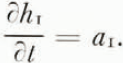
where q 1(x, t) is the perturbation in discharge from the steady datum rate, h 1(x, t) is the perturbation in thickness, and a 1(x, t) is the perturbation in accumulation and ablation rate. B 0(x), c 0(x) and D 0(x) are fixed functions that characterize the particular glacier. B 0(x) is the datum-state width of the channel, c 0(x)/B 0(x) is the velocity of kinematic waves of q 1 down the glacier, and D 0(x)/B 0(x) is their diffusion coefficient. (1) arises from the equation of continuity, while (2) is a consequence of the assumed nature of the flow process. If q 1 is eliminated between (1) and (2) we obtain a type of diffusion equation

where the primes denote differentiation with respect to x.
We shall mostly be concerned with the case where a 1(x, t) is independent of x, so we simply write it as a 1(t) Thus a 1(t) is the function representing the variation in accumulation rate that we are going to try to deduce. It represents the increase in the accumulation rate or the decrease in the ablation rate from the steady state value a 0(x) at any point on the glacier. Other assumptions about the x dependence of a 1(x, t) could be made, but some assumption must be made if the basic problem of deducing budget history from advance—retreat history is to have a solution. Otherwise we should be trying to deduce a function of two variables from a function of only one variable.
The given data, besides the coefficient functions B 0(x), c 0(x), D 0(x) could be the time variations of thickness, that is, of h 1 at some fixed point on the glacier. What is more commonly observed, however, is the variation in the position of the end of the glacier. We denote this by l 1(t), measuring l 1 from the end of the datum glacier. l 1 is geometrically related to h 1 at the wedge-shaped end of the datum glacier (fixed at x = L) by the equation
where θ is the angle of the wedge. The problem is then, given l 1(t), to find h 1(L, t) from (4), and then find what source function a 1(t) in (3) will produce the required h 1(L, t).
3. The use of Influence Coefficients
The record of l 1(t) and therefore of h 1(L, t) is not, in practice, a continuous one. Observations are commonly made at the end of the ablation season at intervals of one year. One way of filling in the gaps in the record would be to make some assumption about the winter-summer variation between the observed points. If we did this our final result for a 1(t) would include the winter-summer variations. We are not usually interested in these, and in any case they would merely reflect what was assumed for the winter-summer variation of l 1(t). To pursue the same line of thought, the true function l 1(t) includes also very high-frequency detail due to individual snowfalls, hot days and so on, and all this is faithfully reflected in the true variation of a 1(t) by the simple relation
We do not have this detailed record of h 1(L, t) nor do we wish to know the corresponding detail in a 1(t) In this situation we propose to adopt a different way of filling in the gaps in the record.
We consider an artificial function a 1(t) that is constant throughout any one (budget) year. It thus consists of a number of steps (Fig. 1a). The corresponding function l 1(t) consists of a number of nearly straight (more accurately, exponential) segments, with discontinuities in slope (Fig. 1b). The observations are taken to be the points p1, p2, p3, .… The method of deducing a 1(t) that we describe is valid when the time Δt = 1 yr. is sufficiently short to be taken as the time interval in a certain finite difference solution of the equations. Now it could happen that a time interval of 1 yr. was loo long for this to be true, but in fact the time constants of glaciers are long enough for the approximation to be a good one. (We verify this later for the individual glaciers treated.) This is a fortunate circumstance for it means that annual observations may be used to infer the step curve of a 1(t). Thus we may say that if the real a 1(t) actually followed the step curve (although we know it does not), then the resulting l 1(t) curve would pass through the observed positions. That is the precise meaning of the a 1(t) step curve that we deduce.

Fig. 1. (a) Assumed step function a 1(t). (b) Resulting response funetion l 1(t)
To a good approximation this step curve may be taken as the mean over the year of the actual a 1(t) function. This mean is closely connected with what is usually, but wrongly, Footnote * called the net budget. The net budget of a glacier at the point x is, in our notation,

where Δt = 1 yr. The second term in the right-hand bracket is what we deduce. When added to a 0(x) and multiplied by Δt it gives the net budget of the glacier at the point in question. In short, the step function a 1(t) that we deduce gives the time variation in the net budget of the glacier.
The numerical method to be described comes from a finite difference approximation to the original differential equations. The time derivative ∂/∂t is replaced by a centred difference using an interval Δt = 1 yr. This means that the equations contain values of the dependent variables at one-year intervals; in particular, they contain the h 1 values at the instants of observation. As we have just noted, Δt = 1 yr. is short enough for this approach to be feasible.
Let the values of h 1 at given x, at intervals Δt, be denoted h(x, 1), h(x, 2), …, back into the past, beginning at a certain instant shown as r in Figure 2. h(x, n) is thus a continuous function of x but a discrete function of time. ‘l’he values of q 1 are similarly denoted q(x, 1), q(x, 2), …. a 1(t), which is now taken as constant over each interval, has values a(1), a(2), …. Note in Figure 2 that these values are placed at the centres of the intervals. We now assume plausibly that
where e(x, 1), e(x, 2), …, are influence coefficients to be determined. Each a(n) in the past, but not in the future, will have an influence on h(x, 1) and since the equations are linear their effects will be additive. This gives equation (5). Equations (6), (7), etc., make the same statement for h(x, 2), h(x, 3), etc., and, since the theory is concerned with small perturbations, they use the same set of coefficients e(x, n).

Fig. 2
We shall show in a moment how the e(x, n) may be computed numerically. For a particular x, which could be x = L we write the equations simply as

If these equations are now solved for a(1), a(2), …, in terms of h(1), h(2), …, we find

where the g(n) are a new set of coefficients which, by substitution in (8), satisfy

Notice that the matrix of g’s in (9) has the same form as that of the es in (8), each row being repeated but displaced by one position.
Equations (10) allow the g’s for a particular x to be found in succession once the es are known, by a simple algebraic process. Equations (9) are the result we need for our problem, for they give the sequence a(1), a(2), …, directly in terms of the observed sequence h(1), h(2), …
The g’s are thus our objective, but to calculate them we must first find the e’s. For this purpose first assume a set of equations for the q’s similar to (5), (6), (7), etc.:

where the f (x, n) are influence coefficients for q. Now write the original differential equation (1) for the point p in Figure 2 and replace ∂h 1/∂t by {h(x, 1)−h(x, 2)}/Δt. Approximate ∂q 1/∂x at p by

where the primes denote differentiation with respect to x. If we now substitute into equation (1), using (5) and (6), and equate coefficients of a(1), a(2), …, we obtainFootnote *

where K(x) = 2B 0(x)/Δt. (14) is thus a finite difference approximation to the original differential equation (1).
Now write the original differential equation (2) for the point r (not p) in Figure 2, substitute from (5) and (11), and equate coefficients of a(1), a(2), …, to obtain

Remembering that all quantities are functions of x and dropping the x’s for brevity, the systems of equations (14) and (15) may be written

where the Z(n), which are functions of x, are given by the recurrence formulae

More compactly we may write (16) as

Eliminating f(n) gives the alternative form
Starting with n = 1 we therefore have a second-order ordinary differential equation to solve for e(x, 1). When this has been done Z(2) may be found from (17), and then (19) with n = 2 gives an equation to solve for e(x, 2), and so on. Thus the influence coefficients e(x, 1), e(x, 2), …, may be computed in succession.
The nature of the above process is made clearer if we notice the physical interpretation of the e(x, n) coefficients. If all the a’s are zero except for a single one, say a(r), which is equal to 1, equation (5) shows that h(x, 1) = e(x, r). Thus e(x, r) is the h 1, response at time 1 to a unit pulse a(r). If a unit pulse of a 1, occurs as shown in Figure 3, the response h 1(t) at given x will be a certain curve. The height of the curve at time rΔt from the beginning of the pulse is e(x, r). In short, the sequence e(x, n) represents the h 1 response at intervals Δt to a unit pulse of a 1. Similarly the sequence f(x, n) represents the impulse response of q 1.

Fig. 3. Interpretation of the influence coefficients e(x, r) as the response to a unit pulse
The same interpretation follows in the continuous case (Δt→0). Here, by analogy with (5) we should write the integral equation

If we apply a unit pulse (Dirac δ-function) of a 1 at time t−t 0, the only contribution to the integral comes from τ = t 0, and we obtain
Thus e(x, t 0) is the response h 1 at time t to a unit pulse that occurred at time t−t 0. Similarly for f.
Accordingly, if we wished to find the continuous function e(x, τ) we should try to solve equations (1) and (2) for an impulse of a, occurring at time t = 0, say. Hence we should wish to solve the equations

for initial condition e = f = 0, where we have simply put e for h 1 and f for q 1 in (1) and (2).
Now our equations (18) are merely a finite difference form of this pair of equations. If a rectangular pulse of unit height is placed in the first interval (Fig. 3) and if ∂f/∂x is approximated by
So far only t has been put in discrete steps, not x. If, however, we write the simplest type of central difference for the x derivatives in (18) we find we have precisely the Crank—Nicholson scheme for integration of the diffusion equation (Reference Crank and NicholsonCrank and Nicholson, 1947; Richtm)er, 1957, p. 93). This is in fact the scheme we have used.
4. Boundary Conditions
It was shown [Nye II, III] that the functions B 0(x), c 0(x), D 0(x) that characterize the glacier may be taken to have the following behaviour at x = 0 and x = L, the end points of the datum glacier: near x = 0, B 0 non-zero, c 0 ~ x, D 0 ~ x 2; near x = L, B 0 non-zero, c 0 non-zero, D 0 ~ L−x. The simultaneous equations (18) for a given n then have the same form as those studied in appendix I of Nye [IV], with e and f substituted for H and Q. From this previous work we know that a unique solution is determined if we require as boundary conditions that e be not infinite at either x = 0 or x = L. This condition at x = 0 is equivalent to the condition f = 0. The boundary condition at x = 0 gives a one-parameter set of solutions which all have the same leading term, namely

Z(n),
c 0,
To summarize, at x = 0 we have a simple condition on e, namely (21); while at x = L we have a condition involving a linear combination of e and e′, namely (22).
5. Solving the finite Difference Equation
Points on the x axis are numbered backwards from j = 1 (x = L) to j = J (x = o) at intervals Δx. In finite difference form equation (19) at any given n is then
where
-
Aj = −aj −γj ,
-
Bj = −2aj −Nj ,
-
Cj = −aj +γj ,
-
aj = (D 0) j /(Δx)2,
-
γj = Vj /2Δx,
-
,

-
,
Thus the coefficients A j , B j and C j in (23) may be computed once and for all; they do not depend on n.
The boundary conditions give, from (21),

and from (22)

To solve the second-order difference equation (23) directly we should need to know two starting values at one end. Instead we have one condition at each end. This boundary value problem is easily dealt with by the method described by Richtmycr (1957, p. 103–04).
We discuss the one-parameter family of solutions S satisfying the boundary condition at x = L (j = 1). They will satisfy a certain first-order difference equation, say
and our problem is to find E j and F j so that (26) is true for any member of S. Since both (25) and (26) are true for all members of S, it follows that

By substituting E j−1 e j +F j−1 for e j−1 in (23) and comparing with (26) we find

Since E 1 and F 1 are now known from (27) these equations allow E 2, E 3, … and F 2, F 3, … to be computed in succession.
Equation (26) may now be used to compute the e j in succession, starting with j = J−1 and using the value of e J given by (24). The method is very efficient.
Accordingly, the numerical procedure is to solve equation (9) by the above method for n = 1. Z(2) is then found from (17) and equation (19) is solved for n = 2, and so on. This determines the e(x, n).
Some methods of this sort for solving the diffusion equation by forward integration in time suffer from instability when the time step is too long in comparison with Δx (Reference RichtmyerRichtmyer, 1957, p. 9). However, the Crank-Nicholson method, which we are using, is unconditionally stable. This important result was secured essentially by taking central differences at p in Figure 2 rather than, say, one-sided time differences at r.
We have now described how, from the functions B 0(x), c 0(x), D 0(x), the influence coefficients (ex, n) in equations (5), (6), (7), etc., may be obtained numerically—essentially by forward integration of the diffusion equation in time steps of 1 yr. The next step is to invert the e array by equations (10) and thus obtain the g’s. This need only be done for the point x that is of interest, normally x = L, the end of the datum glacier. Having found g(1), g(2), …, they may be applied directly to a record of the changes in terminus position to deduce the time variation of the net budget.
A check on the values obtained for the e(n) and g(n) may be made by considering the case of a perturbation steady in time. Thus if a 1(t) = A say, h 1 , will come to the steady state H(x) say. ln the notation of Nye [III] we have
In the notation of this paper, we put
in equations (8) and (9) to obtain

Thus

If μ 0(x) and λ 0(x) are known by some other method (for example by integration of equations (1) and (2) with ∂/∂t = 0, or from the frequency response at zero frequency) these formulae give a check on the values of e(n, x) and g(n, x).
Interpretations may also be given of the other coefficients μ 1, μ 2, … and λ 1, λ 2, … introduced in Nye [III]. For example, take the series
and let h 1 = pt, where p is a constant. Then, at t = 0,
But by (9) we find for a 1 the expression
Hence

In general, by putting h 1 = ptm we find

A similar equation relates μ m with the e(n).
A remark about the convergence of the two series (8) and (9) is in place before we proceed to the numerical work. Experience with the response of the special model [Nye II] leads us to expect that the impulse response of a glacier will persist for several hundred years. Thus several hundred e(n, x) will be needed if (8) is to be used. On the other hand, we found [Nye II] that only a much shorter past history of h 1 was needed in calculating a 1. So we expect that the g series in (9) will converge much more rapidly than the e series in (8). To calculate, say, the first 50 g’s we do not have to calculate more than the first 50 e’s. Even though at n = 50 the e’s are still very appreciable, we expect that the g’s will be quite small.
Let us now sec how these procedures work out in practice.
6. Application to South Cascade Glacier
(i) Computing the influence coefficients
The above method for finding the e(n, x) and g(n, x) was programmed for an I.B.M. 709 digital computer. The functions B 0(x), c 0(x), D 0(x) could be read in in tabular form and the programme made linear interpolation as necessary. The range of x was divided into 500 intervals and Δt was taken as 1 yr. The B 0(x), c 0(x), D 0(x) functions for South Cascade Glacier, Washington, U.S.A. have been derived [Nye III] from the field observations of Reference Meier and TangbornMeier and Tangborn (1965). They gave the values of the e(n) and g(n) at x = L shown in Table I and plotted in Figures 4a and b. The impulse response e(n) behaves as expected (Fig. 4a). We recall that e(n) is the response of h 1 to a pulse of a 1 of unit amplitude, say 1 m./yr., lasting for 1 yr. from n = 0 to n = 1. One year after the start of the pulse h 1 = 1.084 m. The pulse now ends. After a further year h 1 = 1.275 m. and so on down the table. The fact that h 1 grows at first, rather than decays, is the instability phenomenon treated in Nye [I]. The annual increment in h 1 also grows at first, becomes a maximum between n = 6 and 7, and then diminishes. h 1 itself reaches a flat maximum of 4.967 m. at n = 23—the maximum of the flood wave—and then slowly diminishes. Its fastest rate of fall is at n = 43 to 44. After too years, h 1 is still quite appreciable, 0.622 m. This, remember, is the result of a mere 1 m. of ice added to the glacier 100 yr. previously.
Table I Values of e(n) and g(n) for Soute Cascade Glacier and Storolaciaren


Fig. 4a. Influence coefficients e(n) for the termini of South Cascade Glacier and Storglaciaren. The curves also represent the response to a unit pulse

Fig. 4b. Coefficients g(n) for South Cascade Glacier. The coefficients are shown as a step curve to emphasize their interpretation as a series of a(n). Scale at left refers to filled-in curve. The unfilled-in curve (scale at right) shows the same data with scale enlarged 20 times

Fig. 4c. Same as Figure 4b, but for Storglacidren. Scale at left refers to filled-in curve. The unfilled-in curve (scale at right) .shows the same data with scale enlarged 4o times
The behaviour of g(n) is more complicated (Fig. 4b). g(1) = 0.922 and g(2) = −1.085. After this the variation settles down to an oscillation of decreasing amplitude. The g’s diminish much faster than the e’s, as forecast; after n = 46, |g(n)| < 0.00001. The values of g(1) and g(2) may be understood by considering the artificial situation where the glacier was a perfect integrator. Then all the e(n) would be simply Δt( = t). a, would then be ∂ h1/∂t or a(1) = {h(1)−h(2)}/Δt. Comparing with equations (9) we see that
Thus the departures of g(1) and g(2) from the values t and —1, and the subsequent oscillations of g(n), measure the extent to which the glacier is not a perfect integrator.
It is also illuminating to notice that after a pulse of unit height and length Δt the thickness of new material added to the glacier is Δt. Hence as Δt→0, e(1) and e(2) both approach Δt. It then follows from the first two equations of (10) that g(1)→(Δt)−1 and g(2)→(Δt)−1 (In the continuum limit the g’s in fact involve the first derivative of a s-function.)
The physical meaning of the g(n) sequence is found by regarding the g(n) as a series of a1 values moving forward in time. The g(n) sequence represents that time sequence of a 1 which would be necessary to produce a time sequence of h 1in which the first value was 1 and all others were zero.
As a check on the numbers obtained for the two sequences we find

compared with
[Nye IV, table I, col. (2)]. The first too terms thus give excellent agreement with equation (28) for the g’s; but, as is clear from their slow rate of decay, more than ion e’s would be needed before their sum attained the limiting value μ 0 to 3 figures.
As a check to see whether Δt = 1 yr. was small enough the time interval was halved, but the pulse length was kept the same, now running from n = 0 to n = 2. This showed that the e(n) computed with Δt = 1 yr. do indeed represent the true response to a unit rectangular pulse of duration 1 yr. to an accuracy of 0.3 per cent. We conclude that the basic premise, that we can work solely with annual values, is justified.
(ii) Application of the g(n) to the terminus record
The record of the position of the terminus of South Cascade Glacier (Reference Meier and TangbornMeier and Tangborn, 1965) (Fig. 5a) consists of observations in 1928,Footnote * 1953, and annually from 1955–63. The total length is thus 35 yr. The record of a 1(t) (shown shaded in Figure 5b)Footnote † extends from 1952 to1963 with a gap for 1953/54. It is not unreasonable to apply the foregoing theory and see to what extent the theoretical a 1(t) agrees with that observed. (Some comparison has already been made in Nye [III].)

Fig. 5a. Record of terminus position of South Cascade Glacier.● observed positions (Reference Meier and TangbornMeier and Tangborn, 1965), ○ interpolated positions

Fig. 5b. South Cascade Glacier. Time variation of net budget. Shaded step curve: observed, inferred from data of Reference Meier and TangbornMeier and Tangborn (1965). Unshaded step curve: computed from unsmoothed terminus record

Fig. 5c. South Cascade Glacier. Time variation of net budget. Dots show 10 yr. running means of values computed from terminus record; open circle, observed 9.yr. mean
We must first fill in the gaps in the terminus record l 1(t); this was done arbitrarily by linear interpolation for the years 1929–52 and for 1954. The record was also extrapolated back linearly before 1928. The angle θ in equation (4) was taken as the current value of 6.7 degrees. Then the g(n) gave the record of a 1 by equations (9); it is shown in Figure 5b (unshaded). There is some correspondence with the observed a 1 record but it is not at all good; peaks occur in the right places, but they are all accentuated. The best agreement would be expected for the most recent points; detailed agreement ought to fall off into the past as the amount of information in the terminus record diminishes. On this basis the 1962/63 value is discordant. (The theoretical values for 1953/54 and 1954155 are replaced by their mean because separately they depend heavily on the missing l 1 value for 1954.) The computed a 1(t) before 1953 is linear and reflects the assumed linear retreat.
We have given the direct comparison between theory and observation. Now we must look a little more closely at possible sources of difficulty. To begin the discussion let us take note of the following well-known relation which must hold at the terminus of a glacier ending on land:
where

Fig. 6. South Cascade Glacier. Showing the poor correlation between
Now South Cascade Glacier ends in a small lake, and it may be that this is the main cause of the scatter. For, in the first place, the occasional calving of the glacier into the lake causes abrupt changes in the terminus position; secondly, the geometry of the terminus does not strictly fulfil the conditions assumed in the derivation of equation (29). In these circumstances the proper comparison to make would be with the changing height of the ice surface at a transverse section near the terminus, rather than with the changing terminus position, if these data were available for a sufficient number of years. Unfortunately they are not. Thus, the relevance of the theory to the existing data on year-to-year changes of this particular terminus is questionable. The calculation of a 1 with the g coefficients depends heavily on the current retreat rate; it is therefore not surprising that the correspondence in Figure 5b is rather poor.
Although it is evident that the details of the retreat curve cannot be used with much confidence, the average retreat rate over say 10 yr. is surely still significant. With this thought we have taken 10 yr. running means of the computed a 1 values. They are plotted on Figure 5c. For comparison we show the measured 9 yr. mean for 1954/55–1962/63. The agreement is very good. With the short terminus record of South Cascade Glacier we cannot go much further than this, except to deduce that on average the net budget was only very slightly negative in the 1930’s and 1940’s. It seems that for year-to-year fluctuations the geometry of the terminus and calving prevent effective use of the theory. But for longer-period trends the comparison between observation and calculation is favourable for the theory.
7. Application to Storglaciaren
(i) Computation of the influence coefficients
In Nye [IV] the observations of Dr. V. Schytt and Dr. E. Woxnerud on Storglaciären, Kebnekaise, Sweden, were used to deduce B 0(x), c 0(x) and D 0(x) for this glacier. These tabulated functions were then used to find the e(n) and g(n) at the snout of Storglaciären shown in Table I and in Figures 4a and c. The general behaviour of e(n) is the same as we have already seen but the time scale is about twice as long. The maximum of e(n), the peak of the flood wave, is reached at n = 48 (n(48) = 7.100) instead of n = 23 for South Cascade Glacier. The check whether Δt = 1 yr. was small enough for e(n) to be a true representation of the impulse response showed that the maximum error was 0.08 per cent; the figure for South Cascade Glacier was 0.3 per cent; the smaller value for Storglaciären again reflects its longer time-scale.
The g’s (Fig. 4c) do not fall off as fast as one would wish:

The error incurred by not using enough g’s depends, of course, on the record of h 1; but if the record were steady we should obtain 0.0014 h 1 instead of 0.0017 h 1 as the value of a 1, an error of 18 per cent.
(ii) Application to the terminus record
The terminus record of Storglaciären (Fig. 7a) goes back to 1897 with annual observations since 1944 (personal communication from V. Schytt; [Reference AhlmannAhlmann and others], [1950]. The record of annual net budget obtained by Dr. Schytt and Dr. Woxnerud (personal communication from V. Schytt) extends from 1945 onwards.
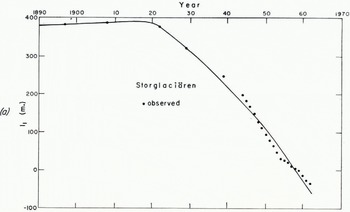
Fig. 7a. Record of terminus position of Storglaciären. Dots show observed positions (personal communication from V. Schytt, [Reference AhlmannAhlmann and others, ] [1950]). Curve shows smoothed position used for computation

Fig. 7b. Slorglaciären. Time variation of net budget. Shaded step curve: observed, inferred from data of Stkytl and Woxnerud (personal communication from V. Schvtt). Unshaded step curve: computed from unsmoothed terminus record

Fig. 7c. Storglaciären. Time variation of net budget. Step curve is computed from the smoothed terminus record. Open circles show 10 yr. running means of observed values
The correlation between a t and

Fig. 8. Storglacicären. Showing the poor correlation between
In this situation it is plain that we must be very cautious in attaching significance to the observed annual fluctuations in
We now wish to compare this theoretical a 1(t) curve with observation. As illustrated in Nye [IV], the observed a 1(x, t) shows some dependence on x from year to year on Storglaciären, although when averaged over several years the approximation a 1(x, t) = a 1(t) is roughly obeyed. The question arises therefore of how best to interpret the a 1(t) of the theory in this case. One way is to take it as an average down the glacier. However, it seems better to take it as the a 1(t) measured at the terminus. By doing this we preserve the theoretical correlation between rate of retreat and ablation rate at the terminus for short-period changes—and for long-term changes it does not matter what point on the glacier is chosen for measuring a 1(t). In this way we may hope to make use of the short-period information in the computed a 1—which we should otherwise have to discard as not meaningful. Accordingly, the a, values shown in Figure 7b as observed (shaded step curve) are in fact a 1 at the current glacier terminus. There is some relation between observed and calculated values. That the relation is not closer we believe to be due primarily to the difficulty of measuring
Again, as with South Cascade Glacier, it seems we must attach little weight to the annual fluctuations of
One complication should be mentioned (personal communication from V. Schytt). Our theory assumes that the slope of the bed is much the same at the successive positions of the terminus. Before about 1935–40 the slope of the bed was in fact opposite in sign to the slope of the ice surface; subsequently it was the same. The main effect, presumably, will be to make θ larger for the earlier years than the value we have taken. Thus, for these years, we have underestimated the absolute magnitude of a 1.
Our conclusion is that, just as for South Cascade Glacier, the observed year-to-year fluctuations of the terminus cannot be used with any certainty to obtain the annual budget; but the general trend of advance and retreat over longer periods gives a mean a 1 that agrees well with recent observation. We therefore think that the curve in Figure 7c, with its maximum in the 1930’s, has genuine significance, and extends the budget record back into the period before it was measured. In saying this we must repeat the proviso that the curve necessarily becomes less trustworthy as it goes into the past.
8. Acknowledgements
I must again express warm thanks to Dr. V. Schytt, Dr. E. Woxnerud, Dr. M. F. Meier and Mr. W. Tangborn for making available their observations before publication. Dr. Schytt and Dr. Meier have also reviewed the manuscript most helpfully—but, naturally, they must not be held responsible for its shortcomings. Most of the computations were done on the I.B.M. 709 digital computer at Yale University; a few were done on an I.B.M. 7094. digital computer at the University of California at Los Angeles.


