


1. INTRODUCTION
In a nearly global context of glacier shrinkage in response to climate change, many glaciers are losing ice volume through increased melt, hence contributing to sea-level rise (Hock and others, Reference Hock, de Woul, Radić and Dyurgerov2009; Jacob and others, Reference Jacob, Wahr, Pfeffer and Swenson2012; Gardner and others, Reference Gardner2013). The large glaciers and ice masses in the Southern Patagonian Andes are no exception (Rignot and others, Reference Rignot, Rivera and Casassa2003; Rivera and others, Reference Rivera, Casassa, Bamber and Kääb2005, Reference Rivera, Benham, Casassa, Bamber and Dowdeswell2007; Chen and others, Reference Chen, Wilson, Tapley, Blankenship and Ivins2007; Ivins and others, Reference Ivins2011). Both the Northern and Southern Patagonian Icefields (hereafter NPI and SPI, respectively) and their outlet glaciers, which have been acknowledged as the largest temperate ice masses in the southern hemisphere (Warren and Sugden, Reference Warren and Sugden1993), have shown high thinning rates since the second half of the 20th century (Rignot and others, Reference Rignot, Rivera and Casassa2003; Willis and others, Reference Willis, Melkonian, Pritchard and Ramage2012a, Reference Willis, Melkonian, Pritchard and Riverab).
Since the 1940s in-situ glacier mass-balance measurements have been carried out on glaciers of various sizes in many glacierized regions worldwide using the traditional glaciological method (Zemp and others, Reference Zemp2015). The WGMS 2013 Glacier Mass-Balance Bulletin dataset contains 37 glaciers for which 30+ observation years are available (WGMS, Reference Zemp2013). The in-situ measurement of glacier mass balance is highly valuable for understanding the processes related to Earth-atmosphere mass and energy fluxes. It is nevertheless a time-consuming and laborious task, and thus cannot be conducted for a large number of glaciers. Moreover, the mass balance of a given glacier may be largely affected by particular topo-climatic factors (glacier size, slope and aspect, wind direction, among others) and consequently, the direct extrapolation of mass-balance measurements to a larger scale must be approached with care (Gardner and others, Reference Gardner2013).
In approximately the last decade, geodetic studies utilizing remotely-sensed data have complemented the in-situ mass-balance surveys, which allow for making wider-scale assessments on glacier changes (e.g. Bolch and others, Reference Bolch, Pieczonka and Benn2011; Nuimura and others, Reference Nuimura, Fujita, Yamaguchi and Sharma2012; Gardelle and others, Reference Gardelle, Berthier, Arnaud and Kääb2013; Kääb and others, Reference Kääb, Treichler, Nuth and Berthier2015 in the Himalaya; Pieczonka and Bolch, Reference Pieczonka and Bolch2015 in the Tien Shan, 2013 Fischer and others, Reference Fischer, Huss and Hoelzle2015 in the Alps or Berthier and others, Reference Berthier, Schiefer, Clarke, Menounos and Remy2010 in Alaska). Though temporally limited by the availability of good quality DEMs, the geodetic mass-balance method provides a more comprehensive and broader overview on the glaciers' state and evolution in comparison with in-situ measurements. Additionally, the geodetic method enables the validation and calibration of mass-balance determinations carried out by means of the glaciological method (Zemp and others, Reference Zemp2013), and is useful to understand the controls of observed glacier changes (e.g. Abermann and others, Reference Abermann, Kuhn and Fischer2011; Carturan and others, Reference Carturan2013; Fischer and others, Reference Fischer, Huss and Hoelzle2015).
By comparing glacier surface topography over different years and making density assumptions to convert ice volume to mass change, the geodetic mass-balance method has become increasingly utilized to derive glacier mass changes. Moreover, co-registration tools have significantly increased the accuracy of this method based on multi-source DEMs, (e.g. Berthier and others, Reference Berthier2007; Bolch and others, Reference Bolch, Buchroithner, Pieczonka and Kunert2008a; Koblet and others, Reference Koblet2010; Lenzano, Reference Lenzano2013; Rastner and others, Reference Rastner, Joerg, Huss and Zemp2016).
The Southern Andes of Chile and Argentina extend for more than 3000 km and host an estimated >29 000 km2 of glacier area (Pfeffer and others, Reference Pfeffer2014). In recent decades, increasingly available satellite imagery has allowed for a better understanding of the current state of glaciers in Patagonia (e.g. Aniya, Reference Aniya1988, Reference Aniya1999, Reference Aniya2001; Aniya and others, Reference Aniya, Sato, Naruse, Skvarca and Casassa1997; Davies and Glasser, Reference Davies and Glasser2012; Bown and others, Reference Bown, Rivera, Zenteno, Bravo, Cackwell, Kargel, Leonard, Bishop, Kääb and Raup2014; Sakakibara and Sugiyama, Reference Sakakibara and Sugiyama2014). Commonly, these studies have mainly focused on glacier area changes, and have shown sustained and widespread glacier wastage (e.g. Schneider and others, Reference Schneider, Schnirch, Acuña, Casassa and Kilian2007; Falaschi and others, Reference Falaschi, Bravo, Masiokas, Villalba and Rivera2013; Masiokas and others, Reference Masiokas2015), and glacier area decline rates of up to ~1% a−1 (see e.g. Paul and Mölg, Reference Paul and Mölg2014). For the Monte San Lorenzo region, which is encompassed within the study area here, Falaschi and others (Reference Falaschi, Bravo, Masiokas, Villalba and Rivera2013) estimated an ice-covered area of ~207 km2 in 2008 and a reduction of 0.8% a−1 between 1985 and 2008.
Glacier length and area changes represent, however, a delayed response to climate change and are affected by debris cover, whereas glacier mass balance is a more direct and immediate response, and offers a more direct assessment of glacier health (Bhattachayra and others, Reference Bhattachayra2016). Yet, in the Southern Patagonian Andes and in terms of glacier mass changes, only the Patagonian Icefields (NPI, SPI and Gran Campo Nevado) have been investigated so far (Möller and Schneider, Reference Möller and Schneider2010; Willis and others, Reference Willis, Melkonian, Pritchard and Ramage2012a, Reference Willis, Melkonian, Pritchard and Riverab). Consequently, little is currently known about glacier mass and volume changes in smaller glaciers across the Patagonian Andes. The state of small alpine glaciers is relevant, since they may contribute to a similar extent to the sea-level rise on a century timescale in comparison with larger ice masses, due to their shorter response time, coupled with large mass turnovers (Radić and Hock, Reference Radić and Hock2011; Marzeion and others, Reference Marzeion, Jarosch and Hofer2012; Gardner and others, Reference Gardner2013; Giessen and Oerlemans, Reference Giessen and Oerlemans2013).
Glacier mass-balance records in the Patagonian Andes remain to this day sparse. It is worth noting that hitherto no glaciological mass-balance programs have been carried out on any of the investigated glaciers of this study. In fact, the closest glacier with long-term measurements, Martial Este, is located more than 850 km to the southeast in Tierra del Fuego (Strelin and Iturraspe, Reference Strelin and Iturraspe2007; Buttstädt and others, Reference Buttstädt, Möller, Iturraspe and Schneider2009). The lack of glacier in-situ measurements for glaciers in southern Patagonia remains so severe for such a densely glacierized area, that it has led to modeling glacier mass losses using energy-balance models (Schaefer and others, Reference Schaefer, Machguth, Falvey, Casassa and Rignot2015).
In view of the above, the main purpose of this study is to focus on the smaller glaciers to the east of the NPI and SPI, by comparing the elevation and mass changes for the same time period (2000–12) as Willis and others (Reference Willis, Melkonian, Pritchard and Ramage2012a, Reference Willis, Melkonian, Pritchard and Riverab). The results are also put into a broader context of glacier mass balance in the Patagonian Andes, thus reducing knowledge gaps in regards to the mass loss of smaller glaciers in the area. We also aim to detect glacier-thinning patterns as a function of a series of glacier morphometric factors (size, slope, orientation, mean elevation) and further analyze the influence of other glaciological characteristics such as debris covers, ice-calving and supra- and proglacial lakes.
2. STUDY AREA
The study area (47°15′S – 49°S, 71°45′W – 73°20′W, Fig. 1) is located in the Southern Patagonian Andes, at the international border between Chile (Región de Aysén) and Argentina (Santa Cruz Province). This region encompasses a large number of alpine-type glaciers located to the east of and in between the NPI and SPI, and also includes the northeastern tip of the SPI and one (Oriental) of its outlet glaciers. The largest glacierized massifs are the Monte San Lorenzo (3706 m, incidentally the highest point in the entire study area) and the Sierra de Sangra range (2200 m) (Fig. 1).

Fig. 1. Average glacier elevation changes for the entire study area. The location in South America is shown in the subset image with a red polygon. NPI and SPI are the Northern and Southern Patagonian Icefields, respectively. The i1–7 symbols correspond to the glaciers also inventoried for the year 2012 (see text for details).
Glaciers in the area show diverse morphologies. While debris-free cirque glaciers are the most abundant type, a minor number of valley glaciers is also present, most notably the Río Oro, Río Lácteo and San Lorenzo Sur glaciers in the Monte San Lorenzo massif. These regenerated valley glaciers are mostly debris-covered and have proglacial lake terminating fronts (Falaschi and others, Reference Falaschi, Bravo, Masiokas, Villalba and Rivera2013).
The climate of this region is modulated to a great extent by the westerly flow, which drives humidity from the Pacific Ocean and produces precipitation maxima during the austral winter months (July–September, Garreaud, Reference Garreaud2009). A strong W-E orographic precipitation gradient characterizes the Patagonian Andes and the eastern steppe-like plains. Precipitation maxima of up to 8–10 m w.e. are found over the SPI, while the easternmost reaches of the Patagonian Andes receive <300 mm a−1 (Villalba and others, Reference Villalba2003). West of the Andean ridge, Garreaud and others (Reference Garreaud, López, Minvielle and Rojas2013) reported a 300–800 mm decrease in annual precipitation over north-central Patagonia for the 1968–2001 period, while to the east of the Andes precipitation changes were deemed not significant by the same authors. Central Patagonia shows a steady warming trend, with episodic cooler periods during the early-mid 1970s and early 21st century (Masiokas and others, Reference Masiokas2015).
While the temperature regime shows less extreme variations, environmental conditions range from fully maritime towards the west to mildly continental on the eastern slopes of the Argentinean Andes. This, in turn, affects mass balance and glacier response to climatic perturbations, since glaciers in more maritime environments will be more sensitive to rising temperatures, as the snow/rain ratio diminishes (Sagredo and Lowell, Reference Sagredo and Lowell2012). Moreover, the variability in climate conditions across the area might result in glaciers of diverse thermal regimes, from temperate in the western flank of the main Andean axis to polythermal towards the eastern side. Incidentally, glacier ELAs lie below 2000 m a.s.l., and glaciers extend far below the 0°C isotherm (Condom and others, Reference Condom, Coudrain, Sicart and Théry2007; Sagredo and Lowell, Reference Sagredo and Lowell2012).
3. DATA
3.1. Satellite imagery
The orthorectified Landsat 7 ETM+ scenes used here (acquisition dates 13 January, 1 and 8 March 2000; paths 231/232, rows 093/094) were obtained from the US Geological Survey (USGS) Earth Explorer portal (http://www.earthexplorer.usgs.gov). A mosaic was generated to exclude any cloud coverage in the individual scenes over the investigated glaciers. Because seasonal snow conditions were not everywhere optimal for glacier mapping (and varied between and within scenes), additional Landsat imagery from 1998 and 1999 (Table 1) was used for further examination of the seasonal snow conditions. In a context of sustained and widespread glacier retreat in the area (Falaschi and others, Reference Falaschi, Bravo, Masiokas, Villalba and Rivera2013; Masiokas and others, Reference Masiokas2015), few if any glaciers were expected to have larger areas in the year 2000 compared with 1999.
Table 1. List of used Landsat imagery
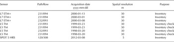
The more recent satellite data originates from a Satellite Pour l'Observation de la Terre 5 (SPOT5) panchromatic image, acquired 8 March 2012. The orthorectified scene was provided by the International Polar Year (IPY) SPIRIT (SPOT 5 stereoscopic survey of Polar Ice: Reference Images and Topographies) project (Korona and others, Reference Korona, Berthier, Bernard, Rémy and Thouvenot2009).
3.2. Shuttle radar topography mission C- and X- band synthetic aperture radar (SRTM) DEM
The Shuttle Radar Topography Mission acquired data continuously between 11 and 22 February 2000 using interferometric synthetic aperture radar (SAR) sensors in C- and X-bands simultaneously (SIR-C and SIR-X, respectively). Void-filled tiles from the SRTM X-band were obtained from the Deutsches Zentrum für Luft und Raumfahrt (DLR) EOWEB Portal (http://www.eoweb.dlr.de) at 1 arcsec resolution. Due to the low acquisition angle of the SRTM X-band, portions of the study area were not covered by the sensor and are therefore not comprised in the distributed elevation grids. These were filled using SRTM C-band grids, in such a way that each glacier polygon contained elevation data from either one SRTM band or the other, but in no case from both of them. The non void-filled SRTM C-band DEM was obtained from the USGS Earth Explorer Portal (http://www.earthexplorer.usgs.gov), also at 1 arcsec resolution. In the following, we use the term SRTM when referring to the SRTM X DEM.
Elevation values in the SRTM C-band products refer to the EGM96 (Earth Gravitational Model 1996) geoid, whereas the SRTM X-band tiles refer to the WGS84 (World Geodetic System 1984) ellipsoid. To obtain scientifically sound elevation and mass-balance changes by means of DEM differencing, all the elevation data must be projected in the same vertical datum. This concern was resolved during the co-registartion procedure described in Section 4.3.
3.3. Satellite Pour l'Observation de la Terre 5 (SPOT5) DEM
A DEM was generated from a high-resolution stereoscopic sensor (HRS) SPOT5 stereo-pair that was provided by the International SPIRIT project (Korona and others, Reference Korona, Berthier, Bernard, Rémy and Thouvenot2009). The present 40 m spatial resolution stereo-pair was acquired on 8 March 2012 and should therefore fairly reflect the conditions of the end of the ablation period in the Southern Andes. Le Bris and Paul (Reference Le Bris and Paul2015) report an absolute horizontal RMSE of 30 m and a vertical bias between −5.5 and +3.5 m compared with ICESat for their study region in Alaska. Optical DEMs have no uncertainties related to the signal penetration, as do radar-derived DEMs, but are affected by the cloud cover problem and low contrast in shadow and highly reflective snow-covered areas (Pieczonka and others, Reference Pieczonka, Bolch and Buchroithner2011). For full technical details, generation and validation of the SPIRIT SPOT5 products see Korona and others (Reference Korona, Berthier, Bernard, Rémy and Thouvenot2009).
3.4. Ground control points
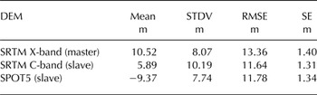
Elevation and slope related biases in mountain areas on SRTM DEMs have been reported by Berthier and others (Reference Berthier, Arnaud, Vincent and Remy2006). Validation and accuracy assessment of SRTM DEMs was carried out by means of independent, field-surveyed GCPs using the Global Navigation Satellite System (GNSS) technique. Selected landmarks were located on rock outcrops, large boulders and road intersections. Successive field campaigns were undertaken in the summers of 2010–12, when 21 GCPs were surveyed with a Trimble 5700 receiver. Additional GCPs were provided by Dr. Robert Smalley from CERI (Center for Earthquake Research and Information, Memphis State University, USA) for a total of 33 GCPs (Fig. 1). The altitudinal range covered by the GCPs spans between 160 and 1700 m. Coordinates of these points were differentially post-processed using data from the private Cochrane GNSS continuous station. The mean horizontal and vertical precisions of these GCPs were 0.34 and 0.37 m, respectively, and were considered sufficient for the purposes of this study.
The independent reference differential GCPs were compared with the corresponding coordinates' elevation values from the SRTM and SPOT5 DEMs and are provided as mean, standard deviation, standard error and RMSE (Fisher and Tate, Reference Fisher and Tate2006) (Table 2).
Table 2. Statistics for the validation of the DEMs against 33 reference GCP points. For a given value, the DEM elevation is subtracted from the GCP elevation
4. METHODS
4.1. Glacier mapping
A new glacier inventory for the year 2000 was prepared using a thresholded ratio Landsat ETM+ image mosaic (e.g. Paul and Andreassen, Reference Paul and Andreassen2009; Bolch and others, Reference Bolch, Menounos and Wheate2010a; Rastner and others, Reference Rastner2012) (Table 1). Bare ice and snow were identified by means of the TM 3/TM 5 band ratio, with a threshold of DN > 2.6 (Racoviteanu and others, Reference Racoviteanu, Paul, Raup, Khalsa and Armstrong2009). Further manual digitizing was necessary for mapping debris-covered ice and ice in cast shadows and for excluding rock outcrops.
For the compilation of our glacier inventory, overall uncertainties were estimated based on the glacier area buffer method as in Bolch and others (Reference Bolch2010b). A buffer size of ±7.5 m for the Landsat ETM+ scenes was selected, leading to an uncertainty of ~5%, which is slightly larger compared with other Landsat inventories (e.g. Paul and Andreassen, Reference Paul and Andreassen2009; Rastner and others, Reference Rastner2012), but may be related to the comparatively small glaciers in our study area. For debris-covered ice delineation on Landsat imagery, it can be assumed that uncertainty in glacier outlines varies by only ~±15 m (Paul and others, Reference Paul2013).
Rolstad and others (Reference Rolstad, Haug and Denby2009) have pointed out that uncertainties in the individual glacier elevation change and mass budget determined using the geodetic method are dependent on the average glacier size. To investigate the resultant differences in the mass budgets, we manually digitized glacier outlines for seven glaciers for the year 2012 based on the SPOT 5 panchromatic scene (Fig. 1). These glacier outlines each represent one of the size classes of the glacier inventory (see Section 5).
4.2. Glacier basins
The method to derive glacier basins builds on those presented by Bolch and others (Reference Bolch2010b) and Kienholz and others (Reference Kienholz, Hock and Arendt2013). The sink-filled SPOT 5 DEM and the manually corrected glacier outlines served as input. In a first step, an ArcGIS model calculates a buffer of 500 m around each glacier polygon and subsets the DEM accordingly. Next, glacier basins are calculated by means of hydrological analysis. Since this procedure leads to many single and often unrealistic basins, the most relevant ones are selected by performing a spatial selection with the help of all the glacier outlines (Bolch and others, Reference Bolch2010b). To automatically merge remaining small basins, we extended the model with the following steps. At the beginning, a buffer of 300 m around all glacier entities is calculated and converted to a raster file. Subsequently outer raster values are lowered by −50 m, which leads to an artificial gutter. Thereafter, the lowest pixel of each gutter per basin is assigned (pour point). The pour points in the following are used for calculating another buffer of 200 m in raster format. With the aid of zonal statistics, a value is allocated to all basins containing the pour point. Finally, all drainage basins having the same ID (received from the pour points) are merged. Since this procedure dissolves only part of the glacier basins a second loop is added to merge more left over single basins.
The main errors of this method are due to DEM artifacts in the glacier accumulation areas, and where small glaciers without a distinct tongue cannot be separated from adjacent, larger glaciers. After the model run, manual corrections of the drainage basins are reduced but nevertheless necessary. We manually improved gross errors with the help of the shaded relief data, flow direction grid and the Landsat scenes.
4.3. DEM co-registration
When quantifying glacier elevation changes by means of DEM differencing, any mismatch in geolocation and/or vertical shift between tiles may result in elevation- or slope-related biases (Nuth and Kääb, Reference Nuth and Kääb2011). Here we have used the procedure of Berthier and others (Reference Berthier2007) to correct misalignments between the SPOT5 DEM and each of the SRTM DEM bands. We found that this co-registration tool showed negligible differences compared with the Nuth and Kääb (Reference Nuth and Kääb2011) procedure in two test areas in the Andes (see also Paul and others, Reference Paul2015).
Before DEM co-registration, both the SRTM C- and X-band tiles were mosaicked and projected in the UTM Zone 18 South projection. Since the SPOT 5 and SRTM C-band products refer to the EGM96 geoid and the SRTM X-band to the WGS84 ellipsoid, all of the elevation grids were put into the same vertical WGS84 datum. We used the SRTM X-band as the main data source as opposed to the SRTM C-band, since the latter penetrates deeper into snow due to its longer wavelength (Rignot and others, Reference Rignot, Echelmeyer and Krabill2001; Gardelle and others, Reference Gardelle, Berthier and Arnaud2012). We calculated the elevation differences between the two SRTM bands over glacierized areas.
In the co-registration process, the master (SRTM) and slave (SPOT5) DEMs were first stacked in a single file, and then projected and resampled to the coarser DEM resolution (40 m here). Subsequently, the slave DEM was iteratively shifted horizontally until a minimum of the standard deviation of the elevation offset was reached.
4.4. Calculation of elevation changes and mass balance
Glacier elevation changes (dh/dt) from February 2000 (t 0) to March 2012 (t 1) were calculated by differencing the SRTM and SPOT5 DEMs. Average dh/dt values for 50 m elevation bins between 300 and 3700 m were calculated from the obtained elevation difference grid to determine the volume changes for each inventoried glacier. Despite the double SRTM coverage, remaining data voids (~30%) over glacierized areas had to be filled to obtain elevation change and volume values for the entire area. The calculated mean dh/dt values of each elevation bin were accordingly inserted into the data voids.
Filling the data voids in the elevation difference grid with the averaged elevation change for each altitude band diminishes the thinning rate (i.e. a more positive value). On the contrary, maintaining the data voids as no data values results in enhanced thinning, an assertion also made by Le Bris and Paul (Reference Le Bris and Paul2015). In order to understand the magnitude by which the mass budget changes between the filled and non-filled difference grids, we calculated the area-averaged mass balance for the raw (non-filled) and void-filled data.
The glacier elevation change values were converted into geodetic mass balance. First, the dh/dt values and glacier area were used to calculate the volumetric ice losses (km3) for the entire glacierized area. Subsequently, we calculated the geodetic mass balance (in m w.e.), assuming an average density conversion factor of 850 ± 60 kg m−3 for all the material involved (Sapiano and others, Reference Sapiano, Harrison and Echelmeyer1998; Huss, Reference Huss2013).
4.5. Uncertainty assessment: DEM differences over non-glacierized terrain
The effects of any systematic shifts between DEMs are minimized in the co-registration procedure, although elevation dependent biases might still be present resulting from the diverse pixel sizes of the different resolution DEMs and the resampling process (Paul, Reference Paul2008; Paul and Haeberli, Reference Paul and Haeberli2008). To account for these elevation- and slope-dependent biases, curvature corrections have been carried out in some cases (e.g. Gardelle and others, Reference Gardelle, Berthier and Arnaud2012, Reference Gardelle, Berthier, Arnaud and Kääb2013). In our case, we did not find any systematic elevation-dependent bias over stable terrain, probably owing to the fairly comparable cell size of the SRTM and SPOT5 DEMs. Although no corrections for elevation-dependent biases have been carried out in this study, pixel values exceeding ±2σ in the difference grid were treated as outliers and were therefore removed.
Elevation differences over stable terrain were calculated in a buffer zone outside the glaciers, of the same area as each glacier polygon. A similar approach, though with a larger mask, was undertaken by Carturan and others (Reference Carturan2013) and Fischer and others (Reference Fischer, Huss and Hoelzle2015). In our study region, implementing exceedingly large buffer areas presents two main inconveniences. (1) Sharp ridges such as lateral moraines (particularly Little Ice Age) have high-frequency slope variations, which coarse DEMs are relatively incapable of reproducing. In such spots, the curvature (first derivative of the slope) is high, and the surface elevation is underestimated in the coarser DEM (Gardelle and others, Reference Gardelle, Berthier, Arnaud and Kääb2013). The effect of different cell size on DEMs will be therefore maximized. (2) Because the radar pulse can be reflected by the canopy surface in forested areas (Sexton and others, Reference Sexton, Bax, Siqueira, Swenson and Hensley2009), the true surface (terrain) elevation might not be adequately captured if the buffer zone extends into densely vegetated areas.
Slope-wise, overly steep areas on stable terrain are not representative of glaciers, which normally have slopes gentler than a given threshold in most of their area (Rolstad and others, Reference Rolstad, Haug and Denby2009). We have therefore excluded them from the uncertainty calculation as follows. The mean slope of the total glacierized area was calculated as 21°, whereas the standard deviation was 12°. Hence, we used a 33° slope threshold and masked the buffer areas around the glaciers with the slope buffers. For the SRTM C-band, the standard deviation σ of the elevation differences with the SPOT5 DEM in the buffered areas was 13.6 m and for the SRTM X-band was 14.1 m.
The distribution of the uncertainty in elevation changes is known to vary depending on the slope, roughness and the presence of low-contrast areas such as deep shadows (Zemp and others, Reference Zemp2013), and uncertainty is expected to increase at higher altitudes. Within the aforementioned buffer areas, the uncertainty was hence first calculated for each of the 50 m elevation bins that cover the 300–3700 m elevation range of the glacier area. For each altitude band, the standard error was calculated following the approach of Gardelle and others (Reference Gardelle, Berthier, Arnaud and Kääb2013):
 $$SE_{\Delta {\rm z}{\rm. rand}} = \displaystyle{{\sigma _{\Delta z}} \over {\sqrt {n_{{\rm eff}}}}} $$
where σ Δz is the standard deviation of the elevation differences between DEMs over stable terrain (Δz) per elevation band and n eff the effective sample size or number of degrees of freedom. N eff is lower than the total number of cells in the off-glacier buffer areas and accounts for the distance of spatial autocorrelation of the elevation differences (Rolstad and others, Reference Rolstad, Haug and Denby2009; Zemp and others, Reference Zemp2013)
 $$n_{{\rm eff}} = \displaystyle{{n_{{\rm tot}}. R} \over {2d}}$$
where n tot represents the total number of cells in each elevation band, R the pixel size (40 m) and d (80 m) the distance of spatial autocorrelation, obtained by means of the Moran's I autocorrelation index (Ruiz and others, Reference Ruiz, Berthier, Viale, Pitte and Masiokas2016).
The mean difference between DEMs over non-glacierized terrain represents the systematic uncertainty for the volumetric changes and can be of negative or positive sign depending on whether it is subtracted or added to the volume balance (Koblet and others, Reference Koblet2010):
 $$\varepsilon _{\Delta z{\rm. sys}} = \displaystyle{{\sum\nolimits_1^n {\Delta z}} \over {n_{{\rm tot}}}} $$
The resultant annual elevation change rate dh/dt is hence expressed as:
 $$\displaystyle{{{\rm d}h} \over {{\rm d}t}} = \displaystyle{{\Delta h_{\rm g} + \varepsilon _{\Delta z{\rm r}..{\rm sys}} \pm SE_{\Delta z{\rm. rand}}} \over {{\rm d}t}}$$
Δz g being the sum of all the elevation difference values for the total glacier area at pixel scale and dt the number of years.
The final random uncertainty for the volume balance (σ vol.rand) results from the cumulated firn density assumptions (σ density.rand) and DEM differences over stable terrain (σ st-terr.rand) as follows (Fig. 2):
 $$\sigma _{{\rm vol}{\rm. rand}} = \sqrt {\sigma _{{\rm density}{\rm. rand}}^2 + \sigma _{{\rm st - terr}{\rm. rand}}^2} $$
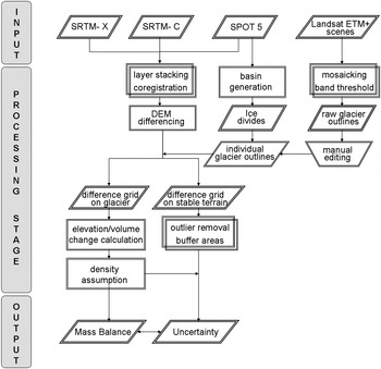
Fig. 2. Schematic workflow and main steps for the retrieval of the mass balance and the associated uncertainty. Parallelogram, data; rectangle, process; inverted trapezium, manual process.
5. RESULTS
5.1. Glacier inventory
We mapped a total of 2253 glaciers larger than 0.01 km2, with an area of 1314 ± 66 km2. The vast majority of the glaciers are relatively small (<0.5 km2) cirque glaciers, the exceptions being the Oriental outlet glacier from the SPI and a few valley glaciers (e.g. Río Lácteo, Rio Oro, San Lorenzo Sur, Narvaez). The largest non-outlet glacier is Calluqueo glacier (50.9 km2), and the mean glacier area is 0.58 km2.
Only the three major valley glaciers in the San Lorenzo massif are debris covered. Coupled with other minor portions of smaller glaciers spread across the study area, the debris-covered ice area accounts for 21.5 km2 (~0.02% of the total glacierized area). The primary source of nourishment of these regenerated glaciers is by avalanche feeding. Debris covers mainly occupy the flat portions of the glaciers, whereas little debris accumulates on steeper glaciers (Frey and others, Reference Frey and Paul2012).
From the total of 2253 inventoried glaciers, merely eight of them are proglacial lake calving (San Lorenzo Sur, Río Lácteo, Narváez, Oriental, three unnamed glaciers in the Narvaez and Gorra de Nieve massifs, and an additional unnamed glacier in the Cerro Penitentes area East of San Lorenzo Sur).
A strong relationship exists between glacier morphology (cirque vs. valley or outlet glaciers) with respect to the distribution of glacier size and number (Fig. 3): ~89% of the investigated glaciers are smaller than 1 km2 and only 2% are larger than 5 km2. Nevertheless, the relative contribution to the total glacier area is 25% for the former and 29% for the latter.
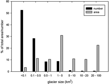
Fig. 3. Percentage contribution to glacier area (grey bars) and number (black bars) per glacier size class.
5.2. Glacier elevation changes and mass balance
The mean, area-weighted elevation change for the entire study area is −0.52 ± 0.35 m a−1, while the total volume loss of the entire study region was of 0.71 ± 0.55 km3 a−1. This yielded a geodetic mass-balance estimation of −0.46 ± 0.37 m w.e. a−1 for the entire area. The raw dh/dt, based on the non-filled difference grid, was determined as −0.6 ± 0.17 m a−1.
The surface elevation of the vast majority of the glaciers (~80%) has lowered between 0 and −2 m a−1 over the 2000–12 period (Fig. 1). Nevertheless, the variability in glacier-specific elevation change within a single mountain ridge was relatively high, as shown in the example of Cordón Gran Nevado (Figs 1, 4). Glacier thinning is greater and more widespread below 1100 m a.s.l. but decreases rapidly with elevation (Fig. 5). Indeed, some elevation gains occur above 3000 m a.s.l. in small parts of the accumulation area of Calluqueo glacier on Monte San Lorenzo (Fig. 4).
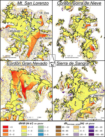
Fig. 4. Detailed view of elevation changes (dh/dt) and DEM differences in meters over stable terrain for four mountain ranges in the study area.
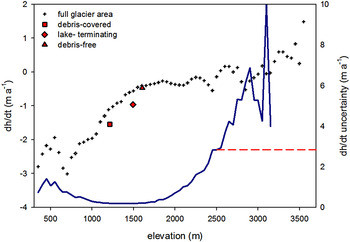
Fig. 5. Mean dh/dt for 50 m elevation bins over the entire glacierized area (black crosses), including the average dh/dt for debris-covered glaciers, square; calving glaciers, diamond; and debris-free glaciers, triangle. The blue line shows the uncertainty distribution with altitude. The uncertainty increases substantially above 2500 m, owed to the impact of DEM artifacts on the decreasing number of off-glacier pixels at higher elevations. For elevation bins >2500 m, a constant dh/dt uncertainty value was used (red dashed line).
Proglacial lake calving glaciers in the area exhibit a relatively wide range of thinning rates, from −0.28 m a−1 for the Narváez glacier to −1.9 m a−1 for Río Lácteo and a mean lowering rate of −0.96 m a−1. Yet, the highest lowering rates among them correspond to lake calving glaciers that additionally have a debris-covered tongue (Table 3). Indeed, and despite the very small proportion of the total glacierized area occupied by debris cover, thinning in the debris-covered portions is greater with respect to both the calving-type and full area averages. A mean dh/dt of −1.54 m a−1 was determined for the debris-covered areas (accounting for 21.5 km2 in total), which is three times that of the entire study area. Discarding the calving and debris-covered glaciers, the averaged lowering rate of the debris-free glaciers is therefore reduced to −0.47 m a−1.
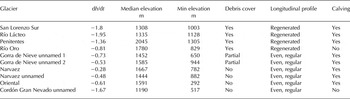
Table 3. Comparison for ten glaciers of topographic and glaciological characteristics with elevation changes
When analyzing the relation between the elevation change rate for individual glaciers and morphometric factors, no strong correlation was found (α = 0.05) for glacier size (r = −0.13) though in general, smaller glacier size classes show a great scatter in dh/dt rates, which is reduced for the larger glaciers (see Fig. 6 and Table 4); correlations were also weak for mean slope (r = −0.11) and median elevation (r = 0.06). The great variability on any of the dh/dt vs. morphometric factor plots is condensed when the data are clustered in 5% quantiles as in Fischer and others (Reference Fischer, Huss and Hoelzle2015). After the mean dh/dt rate is calculated for each of the 20 classes, the relation between thinning rates and the morphometric indices becomes more apparent. Much stronger and significant correlations arise for glacier area (r = −0.62), mean aspect (r = 0.62) and mean slope (r = −0.74), while the weak correlation (r = 0.44) for median elevation was found not to be statistically significant.
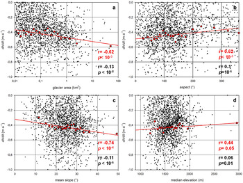
Fig. 6. Average annual elevation changes in m a−1 as a function of glacier morphometric parameters: (a) glacier area (b): mean aspect (c) mean slope and (d) mean elevation. Non-grouped data are shown in black dots and the mean dh/dt rates for 5% quantiles in blue squares. The red trendlines apply to the grouped data.
Table 4. Glacier mean elevation changes and standard deviation per size class
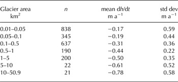
Table 5. Changes in mass balance for seven glaciers as a function of glacier size using the averaged t 0 − t 1 glacier area
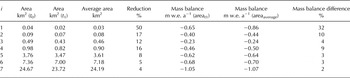
The mass-balance (area t1) column refers to the glacier mass balance considering the glacier size at t 1 (2012), whereas the mass-balance (areaaverage) column corresponds to mass-balance calculation using the averaged 2000–12 glacier size.
6. DISCUSSION
6.1. Variability in glacier elevation change
The elevation change rates of the investigated glaciers might be related to a number of both methodological and glaciological factors and processes. As reported above, most glaciers (80%) in the area have thinned between 0 and −2 m a−1 over the study period. From the remaining 20%, no more than nine glaciers have greater lowering rates, whereas the remaining glaciers show elevation gains.
No positive dh/dt values were found at glacier terminuses, which would indicate advancing fronts or glacier surges. On the contrary, positive dh/dt values are located at glacier limits, mostly below mountain ridges and steep faces that remain in the radar shadow zone, or alternatively, in accumulation areas with low contrast where the optical stereo-correlation fails (Frey and Paul, Reference Frey and Paul2012; Gardelle and others, Reference Gardelle, Berthier, Arnaud and Kääb2013). Most probably, glacier thickening in some units appears as the consequence of DEM artifacts and their increasing effect on the average elevation change of small- to medium-sized glaciers (Le Bris and Paul, Reference Le Bris and Paul2015). In general, the smaller the glacier, the higher the chances for a DEM artifact to considerably alter a glacier's dh/dt rate. The same applies to small glaciers (<0.1 km2) with exceptionally high thinning rates (e.g. −4.11 m a−1, −3.46 m a−1).
The positive elevation changes in the accumulation area of Calluqueo glacier, while spatially limited considering the total glacier area, do not coincide with DEM artifacts. They have nevertheless a relatively large areal extent, enough to be considered as real. Since Monte San Lorenzo is the only massif with elevation exceeding 3000 m a.s.l. it was not possible to identify glacier thickening in the accumulation areas of other large glaciers in other massifs of the study area (see Fig. 5).
In terms of the correlations between elevation change and glacier morphometric indices, the negative dh/dt vs. glacier size correlation indicates that the greatest thinning rates are concentrated on glaciers of relatively large size, i.e. valley glaciers flowing into valleys at low elevation, where temperatures are usually higher than on mountain flanks and ablation is enhanced. On the other hand, the positive correlation between dh/dt and median elevation means that thinning rates tend to be less negative with elevation. Median elevation, in turn, can be taken as a rough proxy for the glacier balanced-budget ELA (Braithwaite and Raper, Reference Braithwaite and Raper2009), which is primarily dependent on continentality. Glaciers in a cooler and moister maritime environment are likely more sensitive to changes in temperature and precipitation compared with those in a warmer, drier more continental regime (Braithwaite and Raper, Reference Braithwaite and Raper2007). Consequently, they are expected to have a more negative mass balance in a warming world (Hoelzle and others, Reference Hoelzle2007).
Further insight into the elevation changes in the region is provided by other glacier characteristics, such as the presence of debris-covered ice, pro- and supraglacial lakes, calving fronts, gradient and flow rate of the lowermost portions of the glacier tongues, and their status as regenerated tongues.
The largest lowering rates are to be found on mostly debris-covered valley glaciers with regenerated tongues and lake terminating fronts (San Lorenzo Sur, Río Lácteo and Penitentes). The San Lorenzo Sur glacier additionally has a large number of supraglacial melt-ponds. While thick (0 to >2 m observed in the field) debris layers should hamper ablation (Benn and Evans, Reference Benn and Evans2010), the presence of pro- and supraglacial lakes has the opposite effect, since they represent heat absorbing spots on the glacier surface (Lüthje and others, Reference Lüthje, Pedersen, Reeh and Greuell2006). Unfortunately, the size of supraglacial lakes on San Lorenzo Sur glacier was too small compared with the 40 m resolution DEMs to establish whether they coincided with enhanced thinning. In contrast, a milder lowering rate was found for Río Oro glacier, which is a regenerated debris-covered glacier, but has a land terminating front and lacks supraglacial ponds. In the Cordón Gorra de Nieve, the mostly debris-free glaciers with calving terminuses have lower thinning rates compared with the aforementioned group of calving, debris-covered glaciers (Table 3), though still higher than the full study area average.
The abundance of land terminating, debris free and non-regenerated glaciers in the area is probably reflected in the mainly lower, total area averaged thinning rate (−0.52 m a−1). Although glaciers with these characteristics and high thinning rates naturally exist, the hypsometric distribution of the individual glaciers is probably the main controlling factor for this major group of glaciers.
The slope and flow rates of the glacier tongues are also related to the process of glacier decline. In general, glacier shrinkage, caused by reduced precipitation and increased ablation, favors the growth and expansion of glacial lakes. Yet on debris-covered glaciers, the process is enhanced by the usually gentle slopes and slow flow rates of the glacier tongues (Quincey and others, Reference Quincey2007). Both field observations and remote-sensing data have in fact demonstrated that the glacier surface gradient provides the boundary conditions for lake formation and expansion, whereas the exact location of lake initiation is mainly controlled by local variations in glacier velocity and surface morphology (Bolch and others, Reference Bolch, Buchroitner, Peters, Baessler and Bajracharya2008b). For the total debris-covered ice area, we calculated an average slope of 11°, whereas the mean slope for the full glacier area is 21°. Although Quincey and others (Reference Quincey2007) have suggested a <2° threshold for lake formation, the proglacial lakes of the Río Lácteo and San Lorenzo Sur are indeed expanding rapidly (Falaschi and others, Reference Falaschi, Bravo, Masiokas, Villalba and Rivera2013), and are most probably contributing to the enhanced thinning of these glaciers.
When looking at the longitudinal profile and hypsometric curves of the San Lorenzo Sur, Río Lácteo and Penitentes glaciers (see Falaschi and others, Reference Falaschi, Bravo, Masiokas, Villalba and Rivera2013), a common feature stands out: most of the glacier area is concentrated at low elevations in gently-sloping tongues. As a result, there is a strong chance for the glacier ELAs to lie above most of the glacier area. This, in turn, might result in low accumulation area ratios (Falaschi and others, Reference Falaschi, Bravo, Masiokas, Villalba and Rivera2013), which are indicative of glaciers in disequilibrium (Bakke and Nesje, Reference Bakke, Nesje, Singh, Singh and Haritashya2011).
6.2. Comparison with the NPI, SPI, Patagonian Andes and other glacierized mountain ranges
The mean dh/dt of −0.52 ± 0.35 m a−1 for the study area is much lower than the extreme average ice surface lowering rates of −1.3 ± 0.1 m a−1 and −1.8 ± 0.1 m a−1 calculated in the same period for the NPI and SPI, respectively, by Willis and others (Reference Willis, Melkonian, Pritchard and Ramage2012a, Reference Willis, Melkonian, Pritchard and Riverab). This means that for exactly the same 2000–12 observed period in this study, the thinning rates of the SPI and NPI are respectively more than triple and double that of the smaller alpine glaciers located further east. At the individual glacier scale, maximum dh/dt rates of −28 m a−1 and up to −57 ± 13 m a−1 were reported for essentially the same time period (Rignot and others, Reference Rignot, Rivera and Casassa2003; Willis and others, Reference Willis, Melkonian, Pritchard and Rivera2012b), which far exceed the more subdued 0 to −2 m a−1 thinning rates found in this study.
At first glance, the above results might surprise, though when seen in terms of glacier morphology and the factors contributing to glacier shrinkage, the interpretation is easier to follow.
The outlet glaciers of the Patagonian icefields are mainly large tidewater and freshwater calving glaciers (glaciers with sea- or lake-terminating snouts such as the Perito Moreno, Jorge Montt, Upsala, Viedma, Pío XI glaciers), which have a cyclic behavior that deviates from the response to climatic variability (Yde and Paasche, Reference Yde and Paasche2010; Wilson and others, Reference Wilson, Carrión and Rivera2016). During this highly dynamic cycle, some calving glaciers may exhibit phases of slow advance or rapid, unstable retreat, the latter accompanied by particularly high thinning rates and calving fluxes (Post and others, Reference Post, O'Neel, Motyka and Streveler2011; Rivera and others, Reference Rivera, Corripio, Bravo and Cisternas2012). The rapid mass loss phase is driven by strong feedback mechanisms between the tightly coupled ice resupply and calving rates. Owing to the highly pressurized subglacial hydraulic systems found in over-deepenings behind the terminal moraines, glacier buoyancy near the terminus is increased, promoting in turn glacier retreat driven by high basal water pressures (Post and others, Reference Post, O'Neel, Motyka and Streveler2011). Certainly, the vast majority of the investigated glaciers in this study have land-terminating terminuses, so their behavior should be largely related to climate forcing and they should have much lower thinning rates. Yet some of them (e.g. San Lorenzo Sur, Río Lácteo, Penitentes), do have (small) proglacial lake terminating snouts, which in turn has led to great iceberg production and rapid frontal retreat (Falaschi and others, Reference Falaschi, Bravo, Masiokas, Villalba and Rivera2013).
Frequently, previously published studies dealing with glacier mass budget around the globe have estimated the mass-balance rates for the Southern Patagonian Andes as a whole, including the SPI and NPI. Ivins and others (Reference Ivins2011) and Jacob and others (Reference Jacob, Wahr, Pfeffer and Swenson2012), to name a few, have estimated the mass balance of the region as −29 ± 10 Gt a−1 (2003–09) and −23 ± 9 Gt a−1 (2003–10). For our comparatively smaller study area, a mass loss rate of −0.6 ± 0.48 Gt a−1 clearly shows that in the Patagonian Andes, ice loss is largely concentrated in the NPI and SPI.
In other mountain ranges around the globe, and in terms of glacier size and morphology, debris cover and latitude, the European Alps host probably the glaciers most similar to those investigated in this study. There, the average mass balance has been much lower for a similar time period than in the Patagonian Andes (−1.06 ± 0.17 m w.e. a−1 (2003–09) Gardner and others, Reference Gardner2013; −2 ± 3 Gt a−1 (2003–10) Jacob and others, Reference Jacob, Wahr, Pfeffer and Swenson2012). Our estimates are nevertheless in accordance with global estimates of −0.55 m w.e. a−1 calculated between 1996 and 2005 (Cogley, Reference Cogley2009) and −0.50 ± 0.04 m w.e. a−1 derived from Gardner and others (Reference Gardner2013).
6.3. Radar penetration and further uncertainty considerations
The Interferometric Synthetic Aperture Radar (InSAR) signal interacts at variable depth with snow, firn and glacier ice, radar penetration depending on the snowpack wetness, radar frequency and wavelength, among others (Willatt and others, Reference Willatt, Giles, Laxon and Worby2010). In the case of SRTM, it has been suggested that the C-band derived DEM may underestimate glacier elevation compared with the X-band, due to the deeper penetration of its radar pulse into the snowpack – several meters) at the 5.6 cm wavelength (Rignot and others, Reference Rignot, Echelmeyer and Krabill2001; Gardelle and others, Reference Gardelle, Berthier and Arnaud2012). Willis and others (Reference Willis, Melkonian, Pritchard and Rivera2012b) investigated the effect of radar penetration in the SPI, finding an average 2 m difference between the two SRTM products.
Also, the radar pulse penetrates much more deeply into dry snow and firn compared with exposed ice (Rignot and others, Reference Rignot, Echelmeyer and Krabill2001). Because SRTM was acquired in mid-winter in the Northern Hemisphere (February 2000), when a substantial yet undetermined amount of fresh snow might have fallen on the glacier surface, some authors have implemented corrections for radar pulse penetration into snow before proceeding with elevation and volume change assessments (e.g. Rignot and others, Reference Rignot, Echelmeyer and Krabill2001; Gardelle and others, Reference Gardelle, Berthier, Arnaud and Kääb2013; Kääb and others, Reference Kääb, Treichler, Nuth and Berthier2015). In the Southern Andes, however, SRTM was acquired during the ablation period, when the glacier surface was ice or wet snow, thus preventing the penetration of the radar wave. Jaber and others (Reference Jaber, Floricioiu, Rott and Eineder2013) confirm in fact that in the accumulation area of the SPI firn was wet during acquisition of the SRTM.
In view of the above, we put the SRTM C- and X-bands into the same vertical datum and performed the co-registration. Although our study area is very close and under similar climatic conditions to that of Willis and others (Reference Willis, Melkonian, Pritchard and Ramage2012a, Reference Willis, Melkonian, Pritchard and Riverab), we found a mean offset of 0.03 m between the SRTM C- and X-bands which, hence, was neglected.
Apart from the uncertainty linked to the scale of the spatial autocorrelation of the elevation differences, Rolstad and others (Reference Rolstad, Haug and Denby2009) also showed that additional systematic uncertainties in geodetical determinations arise from changing glacier areas over the t 0 − t 1 period (Zemp and others, Reference Zemp2013). To investigate this would have required a new inventory for the year 2012, so instead we calculated the mass budget for seven glaciers, each one belonging to one of the size classes of Figure 4, and assuming linear area change over t 0 − t 1 (Table 5). Predictably, the difference in mass budget is greater for the small sized classes than for the larger classes, as a given change in elevation is divided over a smaller area.
Berthier and others (Reference Berthier, Cabot, Vincent and Six2016) and Nuimura and others (Reference Nuimura, Fujita, Yamaguchi and Sharma2012) have also performed GPS surveys to calibrate the source DEMs both on- and off-glacier. Their studies have shown that assessing the uncertainty of geodetic mass-balance determinations purely on the basis of statistical analyses might still not be entirely satisfactory, as the off-glacier bedrock and soil have slopes and roughness unrepresentative of the glacier surface (Rolstad and others, Reference Rolstad, Haug and Denby2009). For an exhaustive analysis of the reservations involved in geodetic mass-balance calculations, it can be argued that additional seasonality corrections should also apply (Fischer and others, Reference Fischer, Huss and Hoelzle2015). In all of these cases, ground truth data, contemporary to the DEM acquisition time, are required, though they are more often than not unavailable.
7. CONCLUSIONS
This study presents a new glacier inventory for the year 2000 and a geodetic mass-balance estimate for the Aysén (Chile) and Santa Cruz Province (Argentina) regions between 2000 and 2012.
We used well-established techniques based on Landsat ETM+ band ratios to map 2253 glaciers and 1314 ± 66 km2 of glacier area.
DEMs derived from the SRTM (2000) X- and C-bands and the SPOT5 HRS sensor (2012) were used to provide individual average elevation changes for the 2253 inventoried glaciers. The results here represent the first regional assessment of glacier elevation and mass changes for this particular region, (and in general for the Chilean-Argentinean Andes beyond the Patagonian Icefields), where detailed, in-situ surveys are scarce or nonexistent.
Precise co-registration of radar (SRTM) and optically derived SPOT DEM elevation grids followed by DEM differencing revealed an area-averaged thinning rate of 0.52 ± 0.35 m a−1. The corresponding volume change of −0.71 ± 0.55 km3 a−1 accounted for a geodetic mass budget of −0.46 ± 0.37 m w.e. a−1 for the entire area.
A relatively high variability in individual glacier response and relatively strong correlations between glacier thinning and glacier slope, size and aspect were found. Our investigations further revealed that the greatest lowering rates occur for lake terminating, debris-covered glaciers, where feedbacks occur between glacier surface lowering, calving processes, the low flow rates and gentle slopes of the glacier tongues and the growth of glacial lakes.
While the mean −0.46 ± 0.37 m w.e. a−1 mass balance is nowhere near the strong thinning rates of the closest glaciers outside the investigated area (NPI and SPI), it nevertheless confirms the general tendency of sustained glacier shrinkage in the area as reported in earlier estimates of glacier areal changes. Moreover, this value is close to the global mass-balance average.
ACKNOWLEDGEMENTS
Data presented in this paper may be obtained by contacting the corresponding author. We acknowledge the Agencia Nacional de Promoción Científica y Técnica (grant PICT 2007-0379) and Consejo Nacional de Investigaciones Científicas y Técnicas for funding this study. E. Berthier and the SPIRIT project kindly provided the SPOT5 DEM and the co-registration tool. T. Bolch and P. Rastner acknowledge funding by the European Space Agency (Glaciers_cci project, code 400010177810IAM). We thank Frank Paul and Michael Zemp (University of Zurich) for their comments on the elevation change accuracy assessment. Ricardo Villalba, Alberto Ripalta, Lucas Ruiz, Aldo Perinetti (IANIGLA) and Leo Montenegro (Parque Nacional Perito Moreno) helped with the survey and processing of ground control points. Alberto Vich helped out with the statistical analysis, and Robert Bruce proofread the manuscript for language checking. Special thanks to Michael Bevis from Ohio State University and Bob Smalley from Memphis State University, USA, for providing the necessary GNSS station data. Finally, we thank Graham Cogley, Neil Glasser and two anonymous reviewers for their valuable comments and suggestions, which led to a much improved final manuscript.


 Open access