


1. Introduction
To predict the effects of climate change and its consequent alterations to water availability in highly populated Himalayan watersheds, it is important to monitor and understand the dynamics of Himalayan glaciers. When measured over long time periods, trends in glacier mass balance can be used as an indicator of climate change (Azam and others, Reference Azam2018; Bolch and others, Reference Bolch, Wester, Mishra, Mukherji and Shrestha2019). Obtaining long-term observations of glacier surface mass balance and other meteorological variables is thus essential to understand linkages between observed glacier changes and their governing atmospheric drivers (Kaser and others, Reference Kaser, Cogley, Dyurgerov, Meier and Ohmura2006). Accordingly, observations from multiple benchmark glaciers in different geographic and climatic regions are needed to better understand the response of glaciers to climate change (e.g. Wagnon and others, Reference Wagnon2007; Fujita and Nuimura, Reference Fujita and Nuimura2011; Sunako and others, Reference Sunako, Fujita, Sakai and Kayastha2019; Wagnon and others, Reference Wagnon2020; Stumm and others, Reference Stumm, Joshi, Gurung and Silwal2021). Although mass-balance studies of Himalayan glaciers have been conducted since the 1970s (Fujii and others, Reference Fujii, Nakawo and Shrestha1976), factors including the remoteness of research sites, harsh weather conditions, financial limitations and time constraints have resulted in discontinuous and spatially non-uniform glacier mass-balance records in this region (Gardner and others, Reference Gardner2013; Azam and others, Reference Azam2018).
Remote-sensing studies reveal that the geodetic mass balance of glaciers in High Mountain Asia (−0.18 ± 0.04 m w.e. a–1 from 2000 to 2016; Brun and others, Reference Brun, Berthier, Wagnon, Kääb and Treichler2017; −0.19 ± 0.03 m w.e. a–1 in between 2000 and 2018; Shean and others, Reference Shean2020) is less negative than the global mean for glaciers (−0.48 ± 0.20 m w.e. a–1 between 2006 and 2016) (Zemp and others, Reference Zemp2019). This offset has mainly been attributed to the slightly positive glacier mass-balance trends experienced in the Karakoram and West Kunlun regions, which are driven by differences in monsoonal and westerly weather patterns (Kääb and others, Reference Kääb, Berthier, Nuth, Gardelle and Arnaud2012; Brun and others, Reference Brun, Berthier, Wagnon, Kääb and Treichler2017; Lin and others, Reference Lin, Li, Cuo, Hooper and Ye2017; Sakai and Fujita, Reference Sakai and Fujita2017; Azam and others, Reference Azam2018).
In situ measurements demonstrate that glacier mass loss is highly spatially heterogeneous in the Himalaya. For example, an extreme mass loss of −0.73 m w.e. at between 2004 and 2014 was reported from ice core measurements at Naimona'nyi Glacier in the western Himalaya at an elevation of 6000 m a.s.l. (Zhao and others, Reference Zhao, Yang, Yao, Tian and Xu2016). In contrast, Mandal and others (Reference Mandal2020) found the mass balance of Chhota Shigri Glacier to be less negative between 2002 and 2019 (−0.46 ± 0.40 m w.e. a−1), despite being situated in the western Himalaya region. Wagnon and others (Reference Wagnon2020) reported that Mera Glacier in the eastern Himalaya lost mass at a moderate rate (−0.41 m w.e. a−1) between 2007 and 2019. However, significantly higher mass losses (−0.80 ± 0.28 m w.e. a−1) have also been reported from the small plateau-type Yala Glacier in the central Himalaya (Stumm and others, Reference Stumm, Joshi, Gurung and Silwal2021). Continuous mass-balance stake measurements (2007–2015) from four glaciers in the Everest region of the eastern Himalaya reveal that the size, shape, elevation and aspect of the glaciers, as well as local climatic influences, are responsible for the heterogeneity in mass balance observed in the region (Wagnon and others, Reference Wagnon2013; Sherpa and others, Reference Sherpa2017). This finding is also supported by other studies across the Himalaya (e.g., Fujita and Nuimura, Reference Fujita and Nuimura2011; Sunako and others, Reference Sunako, Fujita, Sakai and Kayastha2019).
Glacier mass balance also fluctuates seasonally with meteorological conditions in High Mountain Asia. For example, Fujita and others (Reference Fujita and Nuimura2011) showed that fluctuations in annual precipitation and summer air temperatures strongly influenced the annual mass balance of Gregoriev Glacier in the Inner Tien Shan region. Summer temperature and winter precipitation are also the main climatic controls on the mass balance of Chhota Shigri Glacier in the western Himalaya (Azam and others, Reference Azam2014). However, summer temperature has been shown to play no significant role in determining the mass balance of Trambau Glacier in the eastern Himalaya (Sunako and others, Reference Sunako, Fujita, Sakai and Kayastha2019).
A number of studies have tried to reconstruct the long-term mass balance of glaciers in the Himalaya by linking in situ observations with energy-balance and/or temperature-index models (e.g., Fujita and Nuimura, Reference Fujita and Nuimura2011; Azam and others, Reference Azam2014; Zhao and others, Reference Zhao, Yang, Yao, Tian and Xu2016; Sunako and others, Reference Sunako, Fujita, Sakai and Kayastha2019). These studies by examining different glaciers situated across the Himalaya have revealed spatially heterogeneous mass-balance trends that can be used to fill critical data gaps and help to recognize the impact of climate change on Himalayan glaciers.
Rikha Samba Glacier, a benchmark glacier situated in the central Himalaya, has one of the longest in situ mass-balance records of all Himalayan glaciers. Its mass balance has been measured intermittently since 1974 (Fujii and others, Reference Fujii, Nakawo and Shrestha1976; Fujita and others, Reference Fujita, Nakazawa and Rana2001; Fujita and Nuimura, Reference Fujita and Nuimura2011) and has been monitored continuously since 2011 (Stumm and others, Reference Stumm, Joshi, Gurung and Silwal2021). In this study, we first present an update of the in situ mass-balance record between 2017 and 2021. Previous observations extend back until 2017 (Stumm and others, Reference Stumm, Joshi, Gurung and Silwal2021). To bridge gaps in the long-term mass-balance record, we then use a physically based energy-mass balance model which is calibrated using in situ mass-balance measurements to reconstruct the mass balance of Rikha Samba Glacier between 1974 and 2021. Finally, we examine the influence of different meteorological drivers of the glacier mass balance.
2. Study area, data and methods
2.1 Study area
Rikha Samba Glacier (28.82°N, 83.49°E) is a valley-type, debris-free glacier located in the central Himalaya (Fig. 1). This area is situated in an arid region on the leeward side of the mountain range called the Hidden Valley, where high ridges and cliffs constitute challenging barriers to site access (Nakawo and others, Reference Nakawo, Fuji and Shresha1976; Fujita and Nuimura, Reference Fujita and Nuimura2011). The Hidden Valley is one of the driest regions in Nepal. For example, Fujita and others (Reference Fujita, Nakazawa and Rana2001) found that the region received ≈450 mm of precipitation between October 1998 and September 1999. In comparison, annual precipitation is typically <1000 mm a−1 over Nepal's northwestern mountains but can exceed 3000 mm a−1 in central Nepal (Ichiyanagi and others, Reference Ichiyanagi, Yamanaka, Muraji and Vaidya2007).

Fig. 1. (a, b) Location of Rikha Samba Glacier in the central Himalaya delineated by the Randolph Glacier Inventory version 6.0. (c) Rikha Samba Glacier in relation to the mass-balance stake network (yellow circles) and the off-glacier automatic weather station (AWS; blue square and a photo). Glacier elevation contour lines are displayed from the NASA Shuttle Radar Topography Mission digital elevation model (Zandbergen, Reference Zandbergen2008) at 50 m intervals.
Rikha Samba Glacier predominantly faces southeast with a mean slope of 13°. As of 2020, the glacier ranges from 5427 to 6515 m a.s.l. with a total length of ~5.5 km and a planimetric area of 5.62 km2, which makes it the largest and the longest glacier among the ten glaciers situated in the Hidden Valley (Lama and others, Reference Lama, Kayastha, Maharjan and Mool2015). In previous studies, the glacier area was considered to be 4.81 km2 (Higuchi, Reference Higuchi1977; Fujita and others, Reference Fujita, Nakazawa and Rana2001) because they did not consider the full extent of the steep accumulation zone of the glacier. Ground-penetrating radar surveys have revealed that the basal regime of Rikha Samba Glacier is polythermal, consisting mostly of cold ice but with temperate ice in the accumulation zone which is strongly influenced by the percolation of meltwater to the bed through crevasse fields (Gilbert and others, Reference Gilbert2020). This mechanism is currently driving changes to the glacier's thermal regime at over twice the rate that would be possible through advection-diffusion processes alone (Gilbert and others, Reference Gilbert2020).
The first mass-balance measurements of Rikha Samba Glacier were completed in the summer season of 1974 and reported a slightly positive mass balance (Fujii and others, Reference Fujii, Nakawo and Shrestha1976). One-year measurements were also carried out in October 1998 and October 1999 (Fujita and others, Reference Fujita, Nakazawa and Rana2001). Field-based geodetic mass-balance measurements made using rangefinders or differential GPS were conducted between 1974–1994 and 1998–2010. These measurements revealed that Rikha Samba Glacier experienced an overall mass loss between these study periods (Fujita and others, Reference Fujita, Nakawo, Fujii and Paudyal1997; Fujita and Nuimura, Reference Fujita and Nuimura2011). Recent observations between 2011 and 2017 also show a negative mass balance of −0.39 ± 0.32 m w.e. a−1 (Stumm and others, Reference Stumm, Joshi, Gurung and Silwal2021). Temperature and precipitation measurements in the region record monsoonal weather patterns (Shrestha and others, Reference Shrestha, Fujii and Nakawo1976). The region receives high wind speeds (>4 m s−1) during the winter and pre-monsoon seasons, with prevailing northwesterly and southerly wind directions (Shea and others, Reference Shea2015; Gurung and others, Reference Gurung2016). The long-term precipitation and temperature records from the nearby Jomsom area show that this region has undergone increases in average precipitation at a rate of +0.57 mm a−1 from 1957 to 2012, and increases in average air temperature at a rate of +0.023°C a−1 between 1980 and 2012 (Gurung and others, Reference Gurung2016). However, these trends are not statistically significant at the 95% confidence interval (Gurung and others, Reference Gurung2016).
2.2 Observations and data
2.2.1 Meteorological data
An automatic weather station (AWS) was mounted near the Rikha Samba Glacier terminus at 5310 m a.s.l., and has been functioning since 2011 (Shea and others, Reference Shea2015; Gurung and others, Reference Gurung2016). The AWS measures wind speed and wind direction, relative humidity, shortwave radiation, air temperature and precipitation at 15 min intervals (Table 1). Propylene glycol antifreeze was added to the pluviometer to avoid precipitation refreezing inside the instrument. The precipitation recorded by the pluviometer, which does not have a windshield, is affected by precipitation undercatch – the underestimation of precipitation caused by the deflection of dropping hydrometeors away from the inlet of the pluviometer (Sevruk and others, Reference Sevruk, Hertig and Spiess1991; Rasmussen and others, Reference Rasmussen2012; Mekonnen and others, Reference Mekonnen, Matula, Doležal and Fišák2015). If uncorrected, this effect can result in an underestimation of precipitation by up to 10% for rainfall and >50% for snowfall (Ye and others, Reference Ye, Yang, Ding, Han and Koike2004; Wolff and others, Reference Wolff2015; Kirkham and others, Reference Kirkham2019). The quantity of precipitation recorded by the pluviometer was adjusted for undercatch using the correction function from Kochendorfer and others (Reference Kochendorfer2017), which has been shown to perform relatively well for Himalayan environments (Kirkham and others, Reference Kirkham2019). The catch efficiency ratio, C E of the precipitation gauge is calculated from the correlation function, which uses mean air temperature T air (°C), wind speed U (m s−1) and three empirically derived constants (a, b and c), which vary according to the presence or lack of a windshield:

Table 1. Overview of AWS and rain gauge instruments and their specifications

Wind speeds were downscaled from the height of the anemometer to the lower height of the pluviometer orifice using a logarithmic wind profile (Yang and others, Reference Yang, Barry and John1998), accounting for relative changes in gauge height due to snow accumulation. The theoretical catch efficiency of the pluviometer for the typical wind speeds and air temperature conditions recorded at the Rikha Samba Glacier AWS was found to be 57 ± 26% (1σ), which agrees well with previous studies (Ye and others, Reference Ye, Yang, Ding, Han and Koike2004; Wolff and others, Reference Wolff2015). Wind-induced undercatch can therefore result in measurement losses exceeding 50% for solid precipitation at this site.
2.2.2 Reanalysis data
Daily ERA5-Land reanalysis (ERA5L) data, including temperature, precipitation, solar radiation, relative humidity and wind speed at surface level (Muñoz-Sabater and others, Reference Muñoz-Sabater2021), were used to calculate glacier mass balance from 1974 to 2021. Wind speed at a 2 m height from the surface (U) is calculated from wind speed at a height of 10 m in the reanalysis data (U 10), based on the assumption of a logarithmic wind profile (Fujita and Sakai, Reference Fujita and Sakai2014) as described in Eqn (2):

where the surface roughness length (z 0) is assumed to be 0.1 m (Fujita and Sakai, Reference Fujita and Sakai2014).
2.2.3 Observed and gap-filled meteorological data
The AWS has recorded relative humidity, air temperature, solar radiation, precipitation and the wind speed at the terminus of Rikha Samba Glacier since September 2011 with occasional data gaps due to battery failures. To fill the missing input data for the energy-mass balance model, variables from the ERA5L dataset were bias-corrected with the AWS data using linear regression (Table 2). Daily minimum values of each variable measured by the AWS are always higher than the ERA5L data, except in the case of air temperature. Table 2 summarizes the correlation coefficients and the regression parameters between the observed AWS data and the ERA5L data for the period from October 2011 to September 2015. The data exhibit statistically significant correlations for all input meteorological variables and the scatter plots between different variables are presented in the Supplementary Information (Fig. S1). Once correlation was established, the model input data were prepared by filling data gaps with the estimated data for four observation years from October 2011 to September 2015 (Fig. 2). These variables were used as inputs for the mass-balance calculations.

Fig. 2. Meteorological observations gathered by the automatic weather station (AWS) from October 2011 to September 2015. Panels (a) to (e) display daily values of precipitation, incoming shortwave radiation, air temperature, relative humidity and the wind speed, respectively. Grey lines and black lines indicate the observed AWS data and the estimated data, respectively. The estimated data are based on the linear relations presented in Table 2.
Table 2. Parameters used to adjust the daily meteorological variables at the Rikha Samba Glacier AWS

Linear regression (y = mx + c) was used to adjust the variables from the ERA5L data (x). Also listed are the correlation coefficients (r) and the level of significance at the 95 % confidence level (p). The regression equation for precipitation was obtained by the assuming a zero intercept (c = 0).
Daily temperature lapse rates were applied based on the lapse rates observed in the central Himalayan Langtang catchment (Immerzeel and others, Reference Immerzeel, Petersen, Ragettli and Pellicciotti2014). The Hidden Valley does not have sufficient weather stations to calculate the lapse rate using the same methods as used for other more data-rich areas of the Himalaya (Immerzeel and others, Reference Immerzeel, Petersen, Ragettli and Pellicciotti2014; Thayyen and Dimri, Reference Thayyen and Dimri2018). However, similar temperature and solar radiation patterns are observed in both the Hidden Valley and the Langtang catchment (Shea and others, Reference Shea2015).
2.2.4 Mass balance
The mass-balance monitoring program at Rikha Samba Glacier was re-established in 2011 (Gurung and others, Reference Gurung2016; Gilbert and others, Reference Gilbert2020; Stumm and others, Reference Stumm, Joshi, Gurung and Silwal2021) after occasional measurements by Japanese research teams in 1974, 1994, 1998, 1999 and 2010 (Fujii and others, Reference Fujii, Nakawo and Shrestha1976, Reference Fujita, Nakawo, Fujii and Paudyal1997, Reference Fujita, Nakazawa and Rana2001; Fujita and Nuimura, Reference Fujita and Nuimura2011). Since September 2011, mass-balance observations have been conducted using bamboo stakes (Fig. 1) and snow-pit measurements if snow is present. Harsh weather conditions in 2011 and deep snow deposited by Cyclone Hudhud in 2014 made it difficult to access the upper reaches of the glacier in these years. Deep snow also prevented field teams from entering the Hidden Valley through the ‘high-pass’ in 2020 as the field campaign was started 2 months later than usual because of the travel restrictions imposed due to the COVID-19 pandemic. Consequently, no mass-balance data could be collected in 2020.
Mass balance, b o (m w.e.), at a certain stake/point was calculated using changes in stake height, snow thickness and snow and ice densities as:

where ΔS and ΔI are the changes in snow thickness (m) and ice level (m), respectively. ρ s is snow density (302–575 kg m−3) at each snow pit, and ρ i is the assumed density of ice (900 kg m−3; Stumm and others, Reference Stumm, Joshi, Gurung and Silwal2021).
The glacier-wide mass balance, B a (m w.e.), was calculated as:

where s i and S are the area inside a 50 m altitudinal band (m2) and the total surface area (m2) of the glacier, respectively. b i is the mass balance at each 50 m altitudinal interval; this was derived by linear interpolation of the stake mass balance (Fountain and Vecchia, Reference Fountain and Vecchia1999). The equilibrium-line altitude (ELA) was calculated based on the interpolated mass-balance gradients derived from the point measurements (Stumm and others, Reference Stumm, Joshi, Gurung and Silwal2021). The hypsometry of Rikha Samba Glacier was extracted from the NASA Shuttle Radar Topography Mission digital elevation model (Zandbergen, Reference Zandbergen2008) using glacier outlines delineated by Landsat satellite images in 1980, 1990, 2000, 2010 and 2020.
We updated the mass-balance record of Rikha Samba Glacier from an earlier study (Stumm and others, Reference Stumm, Joshi, Gurung and Silwal2021) by presenting data gathered during the 2017/18, 2018/19, 2019/20 and 2020/21 field seasons. As the glacier could not be accessed in 2020, the mass balance for the period of 2019–21 was divided by two to estimate the annual mass balance for the 2019/20 and the 2020/21 seasons.
We used mass-balance data from 2011 to 2021 to calibrate the energy-mass balance model described in Section 2.3. Two distinct mass-balance gradients were observed, characterized by a large gradient in the lower ablation zone and a medium gradient in the transition between the ablation and accumulation zones. Point mass-balance measurements below (above) 5650 m a.s.l. were used to derive the mass-balance gradient over the ablation (accumulation) area.
The uncertainty associated with using point mass-balance measurements was calculated by assessing the random errors accumulated by gathering the stake-height measurements. The point measurement error and the error associated with the interpolation methods chosen were applied for the glacier-wide mass-balance uncertainty (Stumm and others, Reference Stumm, Joshi, Gurung and Silwal2021). The uncertainty of the ELA was estimated by shifting the regression lines of the error range of point measurements as described by Stumm and others (Reference Stumm, Joshi, Gurung and Silwal2021).
2.3 Energy-mass balance model
2.3.1 Description of the model
The daily point mass balance of Rikha Samba Glacier at every 50 m elevation interval was calculated using an energy-mass balance model (Fujita and Ageta, Reference Fujita and Ageta2000; Fujita and others, Reference Fujita, Ohta and Ageta2007, Reference Fujita2011). Previously, this model had successfully estimated glacier mass balance, accumulation area ratio (AAR), ELA and runoff for numerous Asian glaciers (Sakai and others, Reference Sakai, Fujita, Nakawo and Yao2009; Fujita and Nuimura, Reference Fujita and Nuimura2011; Zhang and others, Reference Zhang2013; Fujita and Sakai, Reference Fujita and Sakai2014; Sunako and others, Reference Sunako, Fujita, Sakai and Kayastha2019). The model does not take the aspect or the slope of the glacier into account. The daily sum of precipitation and the daily mean values of air temperature, relative humidity, solar radiation and wind speed are the input variables for the model. It is assumed that the input relative humidity, solar radiation and wind speed are independent of altitude. The energy balance at the glacier surface can be stated as:

where Q M is the heat for snow/ice melting (W m−2). The first three right-hand side components of Eqn (5) represent the radiative flux, where S in is incoming solar radiation, T s is the surface temperature (°C) and α is the albedo of the ice or the snow surface. Incoming long-wave radiation (L in) is calculated using an empirical scheme with relative humidity, air temperature and the ratio of shortwave radiation at the surface to that at the top of the atmosphere (Fujita and Ageta, Reference Fujita and Ageta2000; Fujita and others, Reference Fujita and Nuimura2011). The Stefan–Boltzmann law is used to calculate the outgoing long-wave radiation supposing a black body for the ice/snow surface from modeled surface temperature in Kelvin (T S). σ is the Stefan–Boltzmann constant (5.67 × 10⁻⁸ W m−2 K−4), and ɛs is surface emissivity – which is assumed to be 1.0. Snow-surface albedo on a given day was calculated by assuming an exponential reduction of snow albedo toward a given ice albedo with time after a fresh snowfall, as described by Fujita and Sakai (Reference Fujita and Sakai2014). The surface albedo was calculated following Fujita and Sakai (Reference Fujita and Sakai2014), and depends on the amount of snowfall, the air temperature, the number of days after the snowfall and the minimum albedo of the glacier ice, which is expected to be 0.2 (Fujita and Sakai, Reference Fujita and Sakai2014).
The turbulent sensible (H S) and latent heat (H L) fluxes are calculated using the bulk aerodynamic method as follows:


where c a is the specific heat capacity of air (1006 J kg−1 K−1), ρ a is air density (kg m−3), U is wind speed (m s−1), l e is the latent heat of evaporation (2.50 × 10⁶ J kg−1) and rh is relative humidity. Constant bulk exchange coefficients (C = 0.002) (Kondo and Yamazaki, Reference Kondo and Yamazawa1986) are used as suggested by Fujita and Ageta (Reference Fujita and Ageta2000). Saturated specific humidity (q) is calculated as a function of air temperature (T a) in the model. The surface temperature (T s) is obtained by satisfying Eqn (5) using all of the components (Fujita and Ageta, Reference Fujita and Ageta2000). Q G is sub-surface heat flux. All components are positive when fluxes are directed toward the surface and negative when directed away from the surface.
Most of the precipitation (P p) falls during the monsoon season in the Himalaya (Immerzeel and others, Reference Immerzeel, Petersen, Ragettli and Pellicciotti2014; Shea and others, Reference Shea2015). Precipitation at high elevations can occur as solid (snowfall), liquid (rainfall) and mixed phases (Kayastha and others, Reference Kayastha, Ohata and Ageta1999). It is considered that the possibility of snowfall (P s) or rainfall (P r) depends on the air temperature (T a) (Ueno and others, Reference Ueno1994; Sakai and others, Reference Sakai2006) and affects the mass balance of glacier. This is calculated as:


In this model, the mass balance (b m) at any altitudinal point of the glacier is calculated as follows:

Mass is removed from the glacier as meltwater (Q M /l m) and sublimation (S). Some of the meltwater is retained within the glacier through refreezing (R f). l m is the latent heat for melting ice (3.33 × 10⁵ J kg−1). The extent of meltwater refreezing in the snow layer (R f) is obtained from the change in the vertical ice temperature profile when surface water is present. Further details about these processes can be found in Fujita and Ageta (Reference Fujita and Ageta2000). Their model solves the energy balance and heat conduction in the glacier and calculates the quantity of refrozen water. The amount of refrozen water within the snow is calculated based on snow temperature changes (Fujita and Ageta, Reference Fujita and Ageta2000).
2.3.2 Calibration and validation of the model
Precipitation lapse rate and precipitation ratio were optimized to obtain a good agreement between the observed and modeled mass-balance profiles. The precipitation ratio refers to the change in the original precipitation value with a certain factor (%). Field-based glacier mass-balance profiles from 1998/99 (Fujita and others, Reference Fujita, Nakazawa and Rana2001), 2012/13, 2015/16, 2016/17 (Stumm and others, Reference Stumm, Joshi, Gurung and Silwal2021), 2017/18 and 2018/19 (this study) were used to calibrate the model for the reconstruction of mass balance. These profiles were chosen because only these mass-balance years have point mass-balance data from both the ablation and the accumulation zones, despite the regular measurement program having started in 2011. The mass-balance measurements from 2019/20 and 2020/21 were not included in the calibration since these data are averaged from 2019 to 2021. The model was validated by calculating the glacier-wide mass balance and comparing this to the mass-balance years of 2011/12, 2013/14, 2014/15, 2019/20 and 2020/21 which were not used to calibrate the model. Moreover, the point-to-point mass balance at each stake location was also calculated.
2.3.3 Sensitivity analysis
The sensitivity of the estimated mass balance was calculated by altering the variables and the parameters used in the model individually while the others remained constant. For instance, the precipitation, solar radiation and the relative humidity used in the model were perturbed by ±20%, and air temperature by ±1 K. Similarly, the mass balance was also calculated by changing the minimum value of the glacier surface albedo (α) from 0.2 to 0.4, and 0.2 to 0.0. The critical temperature (CTa) to separate snow and rain was also altered between 1 and 5°C.
3. Results
3.1 Observed mass balance and related variables
The point mass balances as a function of elevation for each observational year using linear regression are shown in Figure 3 (updated from Stumm and others (Reference Stumm, Joshi, Gurung and Silwal2021) with the new mass-balance data from 2017 to 2021). Similarly, glacier-wide mass balance (B a), ELA, AAR and the glacier mass-balance gradients are presented in Table 3. The altitudinal mass-balance profiles of 2017/18, 2018/19, 2019/20 and 2020/21 have similar patterns to previous observational years; glacier-wide mass balance is negative (Stumm and others, Reference Stumm, Joshi, Gurung and Silwal2021). The years of 2017/18 and 2018/19 had mass balances of −0.38 ± 0.26 and −0.26 ± 0.32 m w.e., respectively. In comparison, the annual mass balance for the years between 2019 and 2021 was −0.27 ± 0.36 m w.e. a−1 when averaged over the 2-year period. Averaged annual B a and cumulative B a were −0.39 ± 0.32 and −3.52 m w.e. a−1, respectively, for the one-decade period from 2011 to 2021 (Table 3). All observational years have a negative mass balance except in 2013 (+0.12 m w.e.). Rikha Samba Glacier experienced strong interannual variability in mass balance between 2011 and 2021, fluctuating from the most negative mass-balance year in 2011/12 (−0.72 m w.e.) to a positive mass-balance year in 2012/13 (+0.12 m w.e.), followed by a less negative mass-balance year in 2014/15 (−0.63 m w.e.) (Stumm and others, Reference Stumm, Joshi, Gurung and Silwal2021).

Fig. 3. Hypsometry and observed mass-balance profiles of Rikha Samba Glacier. The hypsometry of the glacier (grey bars) is shown at 50 m elevation intervals. The stake mass balance and its linear regression lines as a function of elevation are shown from the mass-balance years of 1998/99 (Fujita and others, Reference Fujita, Nakazawa and Rana2001), 2011–2017 (Stumm and others, Reference Stumm, Joshi, Gurung and Silwal2021), 2017/18, 2018/19 and 2019/21. The year 2021* refers to the 2-year mass-balance measurement from 2019 to 2021.
Table 3. Updated surface mass balance (B a), equilibrium line altitude (ELA), area accumulation ratio (AAR) and the mass-balance gradients (db/dz) of Rikha Samba Glacier

The vertical gradients of annual mass balance in 2017/18 and 2018/19 for the lower and higher regions of the glacier also vary within the range of previous observations (Table 3). The two-year mass-balance gradient from 2019 to 2021 is quite steep compared to the annual values of the other years presented in Table 3. The mean glacier mass-balance gradient is much greater in the lower area of the glacier (5415–≈5800 m a.s.l.) compared to the higher portion of the glacier (≈5800–5950 m a.s.l.), with a mean value and std dev. of 1.54 ± 0.32 m w.e. (100 m)−1 and 0.46 ± 0.23 m w.e. (100 m)−1, respectively. However, because of the incomplete mass-balance measurements in the upper region of the glacier in 2011 and 2014, the B a calculation for the mass-balance years of 2011/12, 2013/14 and 2014/15 is based on the mean mass-balance gradient of other mass-balance years including 1998/99 (Fujita and others, Reference Fujita, Nakazawa and Rana2001). Accordingly, the B a, ELA and AAR may not characterize the true picture of the glacier health for those mass-balance years. Hence, ELA and AAR of these years are not discussed further here.
The highest ELA was observed in the year of 2015/16 at an elevation of 5870 m a.s.l., followed by the less negative mass-balance year of 2016/17 (5860 m a.s.l). The lowest ELA was observed in 2013 (5725 m a.s.l.). The mean ELA between 2011 and 2021, excluding incomplete mass-balance measurement years, was 5829 m a.s.l. with a std dev. of ±54 m. Similarly, the highest AAR was 0.76 in 2012/13, while the lowest AAR occurred in 2016/17 with a value of 0.4. The mean AAR during the observational period is 0.49 ± 0.14.
3.2 Calibration of the energy-mass balance model
To calibrate the energy-mass balance model, mass-balance calculations were performed using the gap-filled meteorological data for the mass-balance years of 1998/99, 2012/13, 2015/16, 2016/17, 2017/18 and 2018/19. A one-year timeseries for the model is run from 01 October to 30 September of the following year. The precipitation gradient is unknown due to a lack of spatial observations and has stronger vertical dependence compared to other meteorological variables in mountainous regions (Immerzeel and others, Reference Immerzeel, Petersen, Ragettli and Pellicciotti2014; Sakai and others, Reference Sakai2015, Soheb and others, Reference Soheb2020). The energy-mass balance model is sensitive to surface albedo (Fujita, Reference Fujita2008; Johnson and Rupper, Reference Johnson and Rupper2020; Srivastava and Azam, Reference Srivastava and Azam2022), as well as the critical temperature for separating snow and rain (Srivastava and Azam, Reference Srivastava and Azam2022); these uncertainties are assessed in the sensitivity analysis (Section 4.2).
To account for uncertainties related to the precipitation gradient, we investigated the best set of precipitation ratios relative to the estimated precipitation and the elevation gradient of precipitation to yield the best estimate mass-balance profiles for the calibration years. To achieve this, we calculated the root mean square error (RMSE) among the observed and modeled mass-balance profiles during the calibration years (Fig. 4). Based on previous studies in the Himalaya (Immerzeel and others, Reference Immerzeel, Petersen, Ragettli and Pellicciotti2014; Sakai and others, Reference Sakai2015), and the lowest RMSE, we adopted a −15 to 15% km−1 elevation precipitation gradient and a 94–124% precipitation ratio guided by the undercatch predicted to occur in this setting (Section 2.2.1). This is shown by the square box in Figure 4. Values within the boundary of this square box are used for the subsequent calculation of the mass balance of Rikha Samba Glacier.

Fig. 4. Root mean square error (RMSE) of the model performance for Rikha Samba Glacier. RMSE was calculated between the observed mass-balance years of 1998/99, 2012/13, 2015/16, 2016/17, 2017/18 and 2018/19, and the modeled mass balance as a function of the precipitation ratio (horizontal axis) against the estimated precipitation at the AWS location and the elevation gradient of precipitation (vertical axis) for the same period. The ‘+’ sign in the inset box indicates the smallest RMSE.
Observed and modeled mass-balance profiles for the obervational years are shown in Figure 5. The grey lines (based on 961 model runs) enclose the modeled mass balance produced by changing the set of precipitation ratios (94–124%) with a 1% increment against the estimated precipitation at the AWS location and the elevation gradient of precipitation with sequential order from −15 to 15% per km. The red dots with error bars show the observed mass-balance profiles (Figs 5a–k). The modeled mass-balance profiles didn't match well with the observed mass balance for the years 2011/12 and 2013/14 (Figs 5b, d) – particularly in the lower portion of the glacier (5427–5500 m a.s.l.). These patterns are also visible in the scatter plot (Fig. 5l). This tendency may be explained by annual variations in precipitation fall timing and other climatic variables (Sunako and others, Reference Sunako, Fujita, Sakai and Kayastha2019; Zhu and others, Reference Zhu2021). However, the overall agreement between the in situ measurements and the model calculations suggests that the energy-mass balance model is robust enough to estimate the former mass balance of Rikha Samba Glacier.
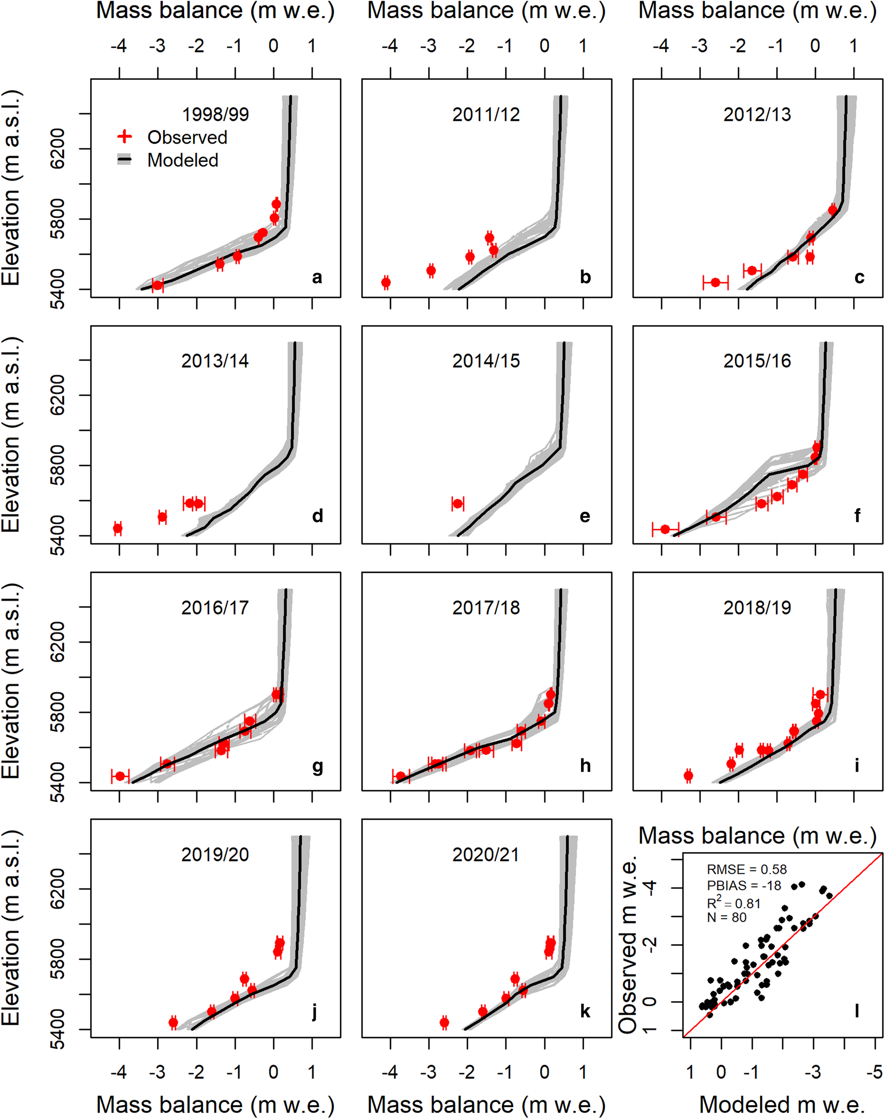
Fig. 5. Observed and modeled altitudinal mass-balance profiles of Rikha Samba Glacier for the periods 1998/99 and 2011–2021. Red dots with error bars are the observed mass balance. Black lines with grey shaded regions, which consist of 961 lines, are the modeled mass-balance profiles produced by the method described in Section 3.2. Graph (l) is a scatter plot between the observed and modeled point mass balance, where RMSE refers to the root mean square error and PBIAS is percentage bias.
3.3 Mass-balance reconstruction
The historical mass balance of Rikha Samba Glacier, reconstructed over 47 years between 1974 and 2021, is displayed in Figure 6. Five different glacier boundaries from 1980, 1990, 2000, 2010 and 2020 were used to calculate the glacier-wide mass balance. The 1980 glacier boundary was used to calculate the mass balance from 1974–1985, and the 1990 glacier boundary for 1985–1995. Similarly, the 1995–2005 and 2005–2015 mass-balance calculations used the 2000 and 2010 glacier boundaries, respectively. The 2020 glacier boundary was used to calculate the most recent 6-year mass-balance data from 2015–2021.

Fig. 6. Comparison between the reconstructed mass balance of Rikha Samba Glacier with field-based observations for the period of 1974–2021. (a) Time series of glacier-wide observed, modeled and geodetic surface mass balance. (b) Observed and modeled equilibrium line altitude (ELA). (c) Annual precipitation (bars) and June–September (JJAS) mean air temperature data (dotted line) at the AWS location which were used to force the mass-balance calculation. The inset plot in (c) shows the average monthly mean air temperature data at the AWS location between 1974 and 2021.
The results indicate that Rikha Samba Glacier has been losing mass at an average rate of −0.56 ± 0.27 m w.e. a−1 throughout the modeled period from 1974–2021. The maximum mass loss (−1.2 m w.e.) was observed in the year of 1976/77, whereas 1974/75 was the most positive mass-balance year (0.1 m w.e.). The average mass-loss rates for the decades of 1974–1985 and 1985–1995 were similar at −0.67 m w.e. a−1. Similarly, mass balance was negative at an average rate of −0.56 m w.e. a−1 between 1995–2005, and 2005–2015, while a mass loss of −0.26 m w.e. a−1 occurred between 2015 and 2021.
For the mass-balance years of 2011–2021, the modeled B a was somewhat less negative than that in the previous decades at −0.35 m w.e. a−1, which is very close to the in situ observations (−0.39 m w.e. a−1) for the same period. A comparison of in situ and modeled B a for the observational years of 2011–2021 is also presented in Figure 6a. The first mass-balance measurement of Rikha Samba Glacier during the summer season of 1974 (Fujii and others, Reference Fujii, Nakawo and Shrestha1976) is also displayed in Figure 6a. However, it should be noted that this measurement is not directly comparable to the annual mass-balance calculation presented here as Fujii and others (Reference Fujii, Nakawo and Shrestha1976) only conducted the mass-balance measurement during the months of July and August in 1974.
The annual variability in mass balance during the reconstruction period is statistically significant (Sen's slope of 0.01, p < 0.01) whereas the input annual precipitation (Sen's slope of 0.67, insignificant at p < 0.01) and the summer air temperature (JJAS; Sen's slope of 0.01, insignificant at p < 0.02) do not experience significant changes over the reconstruction period. The overall mass-balance calculations demonstrate that the glacier mass-loss rate was higher (−0.65 m w.e. a−1) prior to 2000 than in recent decades (−0.47 m w.e. a−1), as shown in Figure 6a. Sunako and others (Reference Sunako, Fujita, Sakai and Kayastha2019) also suggest that greater glacier mass loss occurred prior to 2000 based on a mass-balance reconstruction of Trambau Glacier in the eastern Himalaya between 1979 and 2018. However, an examination of the energy balance records for the entirety of Rikha Samba Glacier (23-elevation interval points) fails to find a statistically significant difference between the time periods before and after the year 2000. A decrease in the total available energy for melt over the entire glacier after 2000 (Table S2) may explain the less negative mass balance in recent decades.
The mean calculated B a for Rikha Samba Glacier between 1974 and 1994 (−0.66 m w.e. a−1) compares well with the geodetic mass balance measured between 1974 and 1994 (−0.57 m w.e. a−1; Fujita and Nuimura, Reference Fujita and Nuimura2011). Similarly, the geodetic mass balance surveyed by Fujita and Nuimura (Reference Fujita and Nuimura2011) was −0.48 m w.e. a−1 between 1998 and 2010; our results estimate a B a of −0.60 m w.e. a−1 for the same period. Gilbert and others (Reference Gilbert2020) found almost the same value for the average mass-balance B a (−0.53 m w.e. a−1) as in our study (−0.60 m w.e. a−1) for the years between 1981 and 2015. The mean ELA for the modeled period (1974–2021) is 5808 m a.s.l., with a std dev. of ±38 m a.s.l. This ELA is comparable to the value calculated by Gilbert and others (Reference Gilbert2020) between 1981 and 2015 (5864 ± 42 m a.s.l.). Overall, the calculated B a and ELA are consistent with observational data and the data from previous geodetic and modeling studies (Fujita and Nuimura, Reference Fujita and Nuimura2011; Gilbert and others, Reference Gilbert2020).
The summer mean (June to September) air temperature (JJAS temperature) for the modeled time period is presented in Figure 6c. These data indicate that at the location of the AWS, positive temperatures are experienced from June to September with a maximum average temperature in July (1.35°C) based on the estimated temperature data from 1974 to 2021. B a variability is correlated more strongly with the annual precipitation than with the mean summer air temperature (Fig. 6c). Based on previous studies in the Tien Shan region (Fujita and others, Reference Fujita and Nuimura2011) and the eastern Himalaya (Sunako and others, Reference Sunako, Fujita, Sakai and Kayastha2019), the climatic variables responsible for driving contrasting annual glacier mass-balance trends differ in space and with the time of year. The same studies show that the summer air temperature is more dominant than annual precipitation in terms of its effect on glacier mass-balance variability. The distinctive characteristics of different glaciers with the response to climate might be associated with the direct alteration of surface albedo and the accumulation of snow on glaciers due to seasonal precipitation patterns, although this factor differs with glacier type and locality (Fujita, Reference Fujita2008; Yamaguchi and Fujita, Reference Yamaguchi and Fujita2013).
4. Discussion
4.1 Spatial characteristics of energy-balance components on mass balance
Boxplots of the mean daily surface energy-balance components of Rikha Samba Glacier in the ablation zone (5450 m a.s.l.) and in the accumulation zone (6000 m a.s.l.), between 01 October 2011 and 30 September 2015, are shown in Figure 7. Overall, the mean daily total available energy (Q M) was positive (25 W m−2) in the ablation zone and was negative (−2 W m−2) in the accumulation zone. The main energy input for both locations is the net shortwave radiation (S net): 125 and 86 W m−2 for the ablation and accumulation zones, respectively. The net longwave radiation energy (L net) constituted a net loss of energy (Litt and others, Reference Litt2019) of ~−77 W m−2 in the ablation zone and −72 W m−2 in the accumulation zone. Mean daily sensible turbulent heat (H s) and latent heat (H L) are positive and negative at both the locations, respectively. On average, a slight energy loss is observed due to the turbulent heat fluxes (H s + H L) in the ablation (−23 W m−2) and accumulation zones (−16 W m−2).

Fig. 7. Average daily surface energy-balance components calculated at the ablation and accumulation zones between 01 October 2011 and 30 September 2015. Each boxplot's boundaries show the upper and lower quartiles, while the middle line of the boxplot shows the median value. Whisker ends indicate the maximum and minimum values.
Similarly, the contribution of melt to the glacier mass balance is analyzed as a case study at both locations for same period. The role of melt in point mass balance at the elevation of 5400 m a.s.l. is substantially higher (75%) than at 6000 m a.s.l., which only contributes ≈4%. Sublimation plays a critical role in regulating the mass-balance changes experienced by Himalayan glaciers. A recent study by Potocki and others (Reference Potocki2022) found that sublimation drives mass loss even at extremely high elevations such as at Mt. Everest's highest glacier (South Col Glacier, 8020 m a.s.l.). Mandal and others (Reference Mandal2022) also observed high rates of snow sublimation while analyzing the 11-year meteorological dataset from the lateral moraine of Chhota Shigri Glacier. The role of sublimation in mass balance is higher at 6000 m a.s.l. (26%) than at 5450 m a.s.l. (10%) for Rikha Samba Glacier. The overall loss from sublimation is 22%, which is similar to other Himalayan glaciers (Srivastava and Azam, Reference Srivastava and Azam2022). Re-sublimation processes also affect the mass-balance trends of Rikha Samba Glacier as we can attribute a 4% and ≈1.5% contribution to positive mass balance in the accumulation and ablation zones, respectively.
4.2 Mass-balance sensitivities
The std dev. for the inter-annual variability of air temperature, precipitation, solar radiation and relative humidity are 0.64°C, 50.60 mm (17.88%), 5.65 W m−2 (2.17%) and 0.02 (4.10%), respectively. The sensitivity of the calculated glacier-wide mass balance to different meteorological variables was examined (Fig. 8, Table S3) by altering the value of precipitation, solar radiation and relative humidity by ±20%, while air temperature was varied by ±1 K throughout the modeled period. All other input variables remained unchanged while perturbing the assigned variable. The average mass-balance change over the modeled period reflects its sensitivity to the perturbations. Mass-balance changes of 0.35 m w.e. a−1 (65%) and −0.44 m w.e. a−1 (−80%) can be expected if we increase or decrease precipitation by 20%, respectively. Similarly, altering the magnitude of incoming solar radiation by ±20% can increase and decrease the modeled mass balance by −81 and 63%, respectively. In general, precipitation and solar radiation have an almost equal influence on mass balance but in opposing directions. Increasing relative humidity by 20% decreases the calculated mass balance by 41%, while mass balance increases by 34% if relative humidity is reduced by the same proportion. B a decreases significantly by −0.69 m w.e. a−1 (−127%) when air temperature is increased by 1 K, whereas B a increases by 0.54 m w.e. a−1 (98%) when air temperature is decreased by 1 K.

Fig. 8. Glacier-wide mass-balance sensitivity to the meteorological variables. Sensitivity was analyzed by changing the quantity of precipitation (P ± 20%), solar radiation (R ± 20%), relative humidity (RH ± 20%) and temperature (T ± 1 K) forcings in the model. The results indicate that the mass balance is more sensitive to changes in temperature than for other variables. The inset map shows the response of the calculated mass balance to perturbations in air temperature and precipitation by increments of 0.5 K from −1.5 to +1.5 K for temperature, and for increments of 10% between −30 and + 30% for precipitation.
Air temperature and precipitation are commonly used to understand the climatic sensitivity of glacier mass balance. We further assess the response of the mass balance of Rikha Samba Glacier to precipitation and air temperature by considering six scenarios in which air temperature is altered in 0.5 K intervals between −1.5 and +1.5 K. Similarly, precipitation is varied by 10% at intervals between −30 and +30%. The mass balance decreased by −194% when air temperature was increased by 1.5 K, whereas the calculated mass balance increased by 133% when air temperature was decreased by the same proportion. The total mass balance varied by ~±35% when precipitation was varied by ±10%. Similarly, the calculated mass balance increased and decreased by 94 and −133% when precipitation was increased and decreased by 30%, respectively.
Taking into account a positive std dev. of the inter-annual variability of air temperature and precipitation such as +0.64°C and +50.60 mm, respectively, the corresponding biases for the resulting change in mass balance were ≈−0.48 and ≈0.40 m w.e., respectively. Similarly, if we consider a negative std dev., the change in mass balance would be ≈0.35 and ≈−0.40 m w.e., respectively (Fig. 8 inset). The inset plot in Figure 8 also suggests that air temperature dominates over precipitation when determining the rate of mass-balance change. Consequently, the negative mass balance reported for Rikha Samba Glacier mostly results from increasing air temperature. This conclusion also supports the results of Che and others (Reference Che2019) for the Urumqi River Glacier No.1 in the Tian Shan region.
4.3 Mass-balance response to parameters
Surface albedo has a strong effect on glacier melting. If the assumed minimum glacier ice surface albedo is increased from 0.2 to 0.4, the glacier mass balance would become more positive by 57%. Similarly, if we assume an ice surface albedo of 0.1, the mass balance would be 31% more negative (Table S4). However, perturbing the maximum critical temperature to separate snow and rain between 1 and 5°C from the reference run of 3°C did not have a hugely significant impact on the modeled mass balance. If a maximum critical temperature of 1°C is assumed, the mass balance would become more negative by −4%, whereas at 5°C a 10% more positive mass-balance change would have been observed.
Furthermore, the impact of using a constant glacier boundary on mass balance was also assessed. If only the recent 2020 glacier boundary is used to reconstruct the mass balance for the whole modeled period, then the mass balance would become less negative by 14%. Similarly, if the 2000 and 1980 glacier boundaries are used, the mass balance would change by −6 and −13% respectively from the present calculation. This consideration is important, as the terminus of Rikha Samba Glacier has continuously retreated since 1974 (Fujita and others, Reference Fujita, Nakazawa and Rana2001; Bajracharya and others, Reference Bajracharya2015; Stumm and others, Reference Stumm, Joshi, Gurung and Silwal2021), reducing the overall glacier area by almost 15% in 40 years between 1980 (6.65 km2, Bajracharya and others, Reference Bajracharya2015) and 2020 (5.62 km2).
Due to the limited duration of the meteorological data, which is less than that required to run a full energy-mass balance model, we instead use the bias-corrected ERA5 and ERA5L data at AWS location for the mass-balance calculation. To determine the applicability of these datasets and the validity of the bias-correction method, we conducted multiple case studies, similar to the method described in Section 3.2, to obtain the lowest RMSE values of the modeled and observed mass-balance profiles for the calibration period. Firstly, the linear bias-correction of the input variables were tested on daily (single equation), monthly, four-season and two-season timescales as shown in Table S1 for each ERA5 and ERA5L dataset. Secondly, the model was calibrated using the bias-corrected data. Finally, the use of ERA5L data with the single linear equation bias-correction method was chosen as it is characterized by the smallest RMSE values among the pre-described condition (Table S2).
4.4 Comparison with other studies
The mass-balance reconstruction presented here provides an opportunity to make comparisons with similar studies that employed melt models integrated with field-based studies in the Himalaya. A mass-balance reconstruction of the monsoon-dominated debris-free Trambau Glacier in the eastern Himalaya was found to be −0.65 m w.e. a−1 between 1979 and 2018 (Sunako and others, Reference Sunako, Fujita, Sakai and Kayastha2019), which is more negative than the rate observed at Rikha Samba Glacier. The modeled and observed mass balances of two small glaciers situated to the east of Rikha Samba Glacier – AX010 Glacier (eastern Himalaya) and Yala Glacier (central Himalaya) – exhibit largely negative mass-balance trends (e.g., Kayastha and others, Reference Kayastha, Ohata and Ageta1999; Acharya and others, Reference Acharya and Kayastha2019) compared to the present study on Rikha Samba Glacier. In addition, a modeling study of Dokriani Glacier from the central Himalaya to the west of Rikha Samba Glacier revealed that this glacier has experienced moderate mass losses with an annual loss of −0.25 ± 0.37 m w.e. a−1 from 1979 to 2018 (Azam and Srivastava, Reference Azam and Srivastava2020).
Model results and field observations at Chhota Shigri Glacier (located ≈680 km west of Rikha Samba Glacier in a monsoon-arid transition climate, western Himalaya) demonstrate that this glacier has experienced a moderate mass loss of −0.30 ± 0.36 m w.e. a−1 between 1969 and 2012 (Azam and others, Reference Azam2014). A study by Soheb and others (Reference Soheb2020) also found that Stok Glacier, a glacier located in the arid western Himalaya, has lost mass at a moderate rate (−0.47 ± 0.35 m w.e. a−1) in the 28 years spanning 1978–2019. Naimona'nyi Glacier in the same region has lost mass at a rate of −0.39 m w.e. a−1 between 2010 and 2018 (Zhu and others, Reference Zhu2021). Another study employing an energy-mass balance model approach to Chhota Shigri Glacier in the western Himalaya and to Dokriani Glacier in the central Himalaya reported mean glacier-wide mass balances of B a −0.31 ± 0.38 and −0.27 ± 0.32 w.e. a−1, respectively, between 1979 and 2020 (Srivastava and Azam, Reference Srivastava and Azam2022).
Comparisons with these studies indicate that the rate of shrinkage of Rikha Samba Glacier is within the observed range of other glaciers in the Himalaya. Greater rates of mass-balance decline are observed for glaciers which are situated further to the east of Rikha Samba Glacier than for those located further to the west. Glaciers in the Himalaya are experiencing heterogeneous mass losses due to contrasting glacier geometries (e.g., elevation difference, orientation, shape and size) and differences in the magnitude and timing of monsoonal precipitation (Fujita and Nuimura, Reference Fujita and Nuimura2011; Yamaguchi and Fujita, Reference Yamaguchi and Fujita2013; Sherpa and others, Reference Sherpa2017).
4.5 Model limitations
Himalayan glaciers exhibit complex dynamics that are simplified in numerical model simulations, so even a small error can have a large effect on the result's confidence (Sauter and Obleitner, Reference Sauter and Obleitner2015). The energy-mass balance model employed in this study works using elevation intervals along the length of Rikha Samba Glacier. Consequently, the model is unable to provide insights into the lateral spatial variability in mass balance across the entire glacier. Additional uncertainty may stem from the off-glacier AWS data used to compute the surface-energy balance of the glacier, as this does not capture the full heterogeneity of the glacier surface and therefore cannot be directly compared to the glacier melt rates (Stigter and others, Reference Stigter2018). Furthermore, the ERA5L data have its own limitations such as a lower spatial resolution when compared to observational data. The model does not include any component of heat sourced from rainfall as this has been previously shown to contribute a minimal amount of energy compared to other radiative and turbulent heat fluxes in the total energy calculations (Kayastha and others, Reference Kayastha, Ohata and Ageta1999; Mandal and others, Reference Mandal2022). The model also does not account for snow deposition and transport due to topography and wind redistribution, which lowers the accuracy of the mass-balance calculations. Finally, although different glacier area boundaries were used to calculate the glacier-wide mass balance for each decade (1980, 1990, 2000, 2010 and 2020), these glacier boundaries are assumed to remain constant when calculating annual mass balances within each respective decade which limits the accuracy of the annual mass-balance calculations.
5. Conclusions
We calculated the annual mass balance of Rikha Samba Glacier from 1974–2021 to fill a large temporal gap in field observations that are available for 1974, 1998/99 and 2011–2021. We also updated the field-based mass-balance measurement until 2021 after the comprehensive documentation of on-going glacier monitoring of this glacier since 2011 (Stumm and others, Reference Stumm, Joshi, Gurung and Silwal2021). We demonstrate that a physically-based energy-mass balance model can reconstruct the surface mass balance of Rikha Samba Glacier using reanalysis ERA5L, AWS, and in situ mass-balance data. The average annual glacier-wide mass balance and cumulative mass balance were found to be −0.56 m w.e. a−1 from 1974 to 2021. The reconstruction demonstrates that Rikha Samba Glacier had a more negative mass balance (−0.65 m w.e. a−1) in the past (1974–2000) compared to the more recent decades (2000–2021, −0.47 w.e. a−1). Sensitivity analysis of the input variables to the mass-balance changes, conducted by perturbing the quantity of precipitation, relative humidity and solar radiation by ±20% and air temperature by ±1 K, shows that mass-balance variability is most sensitive to changes in air temperature.
Supplementary material
The supplementary material for this article can be found at https://doi.org/10.1017/jog.2022.93.
Acknowledgements
We thank the Government of Norway for supporting and funding this research, as well as our national partners, including the Department of Hydrology and Meteorology Government of Nepal (DHM), Water and Energy Commission Secretariat, Government of Nepal (WECS), and Tribhuvan University, Nepal (TU). This study was partially supported by core funds of ICIMOD contributed by the governments of Afghanistan, Australia, Austria, Bangladesh, Bhutan, China, India, Myanmar, Nepal, Norway, Pakistan, Sweden and Switzerland. We acknowledge Tenzing Chogyal Sherpa for making the study area map and his contribution to mass-balance measurement in 2018 along with Dawa Tshering Sherpa. The authors extend a big thanks to all field members, field assistants, porters, guides and special gratitude to Ang Kipa Sherpa, Chyapten Sherpa, Laxmi Kumar Rai and Pemba Sherpa for their support during the glacier measurements, installation and maintenance of weather station and for all of their logistical support. We extend our sincere gratitude to Dorothea Stumm, Bikas Bhattarai, Niraj Pradhananga for the initial mass-balance stake and weather station installation and maintenance, and for their intellectual support. K. Fujita was supported by JSPS-KAKENHI (grant numbers 17H01621 and 18KK0098), and JSPS and SNSF under the Joint Research Projects (JRPs). Finally, we thank the scientific editor, Argha Banerjee, and two anonymous reviewers for thorough and helpful reviews that significantly improved the paper.
Author contributions
T.R.G. and R.B.K. designed the study. T.R.G., J.D.K. and S.P.J. analyzed the data. T.R.G. performed model calculation with the support of K.F. T.R.G., S.P.J., A.S. and K.F. conducted field visits in different periods. T.R.G. wrote the manuscript with the support of all other co-authors.
Data availability statement
The in situ mass-balance datasets are also available from the World Glacier Monitoring Service (WGMS) compiled and edited by Zemp and others (Reference Zemp2021).
Disclaimer
The views and interpretations in this publication are those of the authors and are not necessarily attributable to ICIMOD.


 Open access