


Introduction
Meltwater from the Greenland ice sheet (GrIS) has been one of the major contributors to global sea-level rise in the past few decades (Shepherd and others, Reference Shepherd2012, Reference Shepherd2020; Khan and others, Reference Khan2015). The absorption of solar radiation controls the surface ice melt, which is modulated by the surface ice albedo (SIA) (Box and others, Reference Box2012), defined as the ratio of the total reflected to the total incident solar radiation (Cogley and others, Reference Cogley2011). The SIA of the GrIS has been measured by remote-sensing platforms during the recent decades (Tedesco and others, Reference Tedesco2015; Shimada and others, Reference Shimada, Takeuchi and Aoki2016), and is a critical parameter in current GrIS melt models (van Angelen and others, Reference van Angelen2012; Shepherd and others, Reference Shepherd2012). The darkening of surface ice, which corresponds to a lowering of SIA, increases the absorption of solar radiation (Tedesco and others, Reference Tedesco2016; Box and others, Reference Box, As and Steffen2017; Stibal and others, Reference Stibal2017; Cook and others, Reference Cook2020) and enhances melt rates (Naegeli and others, Reference Naegeli, Huss and Hoelzle2019). Satellite records have shown that the SIA of the GrIS has declined at a rate of −0.028 ± 0.008 decade−1 over the past two decades since 2000 (He and others, Reference He2013). Most distinctive is an area of surface ice with particularly low albedo in the ablation zone along the western margin of the ice sheet, known as the Dark Zone (Knap and Oerlemans, Reference Knap and Oerlemans1996; Wientjes and Oerlemans, Reference Wientjes and Oerlemans2010; Ryan and others, Reference Ryan2018). It often grows to ~20 km in width, extends for several hundred kilometers in length, and is particularly prominent from 65$^\circ$ N to 70$^\circ$
 N (Wientjes and others, Reference Wientjes, van de Wal, Reichart, Sluijs and Oerlemans2011; Ryan and others, Reference Ryan2018).
Satellite imagery is commonly used to examine the albedo of the earth surface, and many albedo products are available, including Moderate Resolution Imaging Spectroradiometer (MODIS) products such as MOD10A1.006 Terra Snow Cover Daily Global 500 m (Hall and others, Reference Hall, Riggs and Salomonson1995, Reference Hall, Salomonson and Riggs2016, Reference Hall2018), which have been widely used in studies of snow and ice albedo (Stroeve and others, Reference Stroeve, Box and Haran2006; van Angelen and others, Reference van Angelen2012; Stroeve and others, Reference Stroeve, Box, Wang, Schaaf and Barrett2013; Shimada and others, Reference Shimada, Takeuchi and Aoki2016). Recently, albedo products have also been derived from the high spectral-resolution sensor on Sentinel 3, which has been operational since 2016 (Wehrlé and others, Reference Wehrlé, Box, Niwano, Anesio and Fausto2021). Longer time series of albedo variations can be obtained by merging data from different products. For example, the Global LAnd Surface Satellites (GLASS) dataset provided a long time series (1981–2019) of albedo by merging albedo retrieved from Advanced Very High Resolution Radiometer (AVHRR) and MODIS (Liu and others, Reference Liu2013).
All albedo products have inherent limitations, because of their differing spatial, spectral and temporal resolution and the active lifespan of the associated satellite. Satellite images with coarser ground resolution (>102 m) effectively average out sub-pixel variations in surface conditions and cannot resolve small-scale spatial patterns of albedo (Ryan and others, Reference Ryan2017). This limits our ability to attribute albedo changes to specific surface processes and therefore our understanding of the mechanisms of surface albedo change. For example, the AVHRR images utilized in the GLASS albedo product have a spatial resolution of 1.1 km. MODIS has a resolution of 500 m for its albedo product MOD10A1.006 (Hall and others, Reference Hall, Riggs and Salomonson1995, Reference Hall, Salomonson and Riggs2016), and Sentinel 3 has a resolution of 300 m, but these are all too coarse to resolve the important 10–100 m scale albedo variations that characterize small-scale, localized melt processes (Naegeli and others, Reference Naegeli, Damm, Huss, Schaepman and Hoelzle2015, Reference Naegeli2017). Better spatial resolution, down to 10–30 m, is available from earth observatory satellites such as Landsat and Sentinel 2. Investigation of historical albedo variations is often compromised by the lifetime of individual satellites, and the launch of new satellites offers new opportunities to extend albedo time series, such as albedo data from Sentinel 3 which became available in 2016. Hence, the marrying together, or harmonization of different remote-sensing products is necessary to produce time series of longer duration.
Here, we aim to maximize the duration and the spatial and spectral resolution of albedo variations in the Dark Zone of the GrIS, by harmonizing Landsat 8 and Sentinel-2 data. The combination of Landsat and Sentinel 2 datasets (Fig. 1a) offers a favorable balance of spatial and temporal resolution. Hereafter, Landsat 4, 5, 7, 8 and Sentinel 2 data will be referred to as L4, L5, L7, L8 and S2, respectively. Landsat provides the most continuous Earth observation record, with imagery dating back to 1972 (Williams and others, Reference Williams, Goward and Arvidson2006; Wulder and others, Reference Wulder2016). S2 imagery has better spatial and temporal resolution than the Landsat series (Drusch and others, Reference Drusch2012; Vuolo and others, Reference Vuolo2016). Merging imagery from multiple earth observation satellites is nuanced, and cannot be undertaken by simply joining the target image collections due to the differences in the spectral response, atmospheric correction, field of view, spectral sensitivities (Fig. 1b), resolutions etc. of the different satellite sensors, known as cross-sensor differences (Roy and others, Reference Roy2016a; Claverie and others, Reference Claverie2018). For this reason, we developed a methodology to harmonize the L4–L8 and S2 data, where ‘harmonization’ is defined here as the minimization of cross-sensor differences via statistical sensor to sensor calibration.

Fig. 1. Availability of Landsat and Sentinel 2 imagery, and the band widths of interest in this study. (a) The timeline of data availability on Google Earth Engine. Data for Greenland from Landsat 4/5 TM were available from 1984, and from the Sentinel 2 Level-2 product during 2019, as shown by black dotted line. (b) Band designations for sensors on Landsat 4/5 TM, Landsat 7 Enhanced Thematic Mapper Plus (ETM+), Landsat 8 Operational Land Imager (OLI) and Sentinel 2 Multi-Spectral Instrument (MSI), adapted from https://landsat.usgs.gov/spectral-characteristics-viewer). Only the bands of interest (blue, green, red, NIR, SWIR1 and SWIR2) are shown here. Spectral wavelength (nm) is indicated by the box length and band names are labeled within the boxes.
Various attempts have been made to harmonize the Landsat and S2 datasets in the past, but none have yet been optimized for the entire duration of L4–L8 and S2 measurements over bare ice- and/or snow-covered ice. For example, Roy and others (Reference Roy2016a) established a statistical approach to harmonize the comparable spectral bands of L7 and L8 images, but these statistical sensor transformation functions were optimized for the mid-latitudes in the conterminous USA (here defined, the 48 adjoining states, excluding Hawaii and Alaska), excluding highly reflective surfaces such as snow. A more recent harmonized Landsat and S2 (HLS) dataset (Claverie and others, Reference Claverie2018) provides seamless L8 and S2 imagery. However, the harmonized dataset starts in April 2013 and does not include any Landsat series data prior to L8, and so commences from April 2013 (Fig. 1a). No study as yet has produced a reliable and efficient method of cross-calibrating Landsat and S2 data to provide a continuous and consistent, harmonized dataset that will enable rapid, yet accurate monitoring and analysis of albedo variations over large areas of ice/snow-covered earth surfaces, such as the ablation zone of the GrIS.
Broadband albedo is defined as the ratio of the total reflected to the total incident solar radiation across the entire electromagnetic spectrum (Cogley and others, Reference Cogley2011). By contrast, the shortwave broadband albedo (SBA) generally used in glaciological remote sensing refers to the commonly measured wavelength range from 400 to 2400 nm only (Lucht and others, Reference Lucht2000). SBA numerically approximates to broadband albedo because this range contains the majority ($> \!99\percnt$ ) of the solar radiation received at the earth surface (Lucht and others, Reference Lucht2000; Naegeli and others, Reference Naegeli2017). Both the Landsat series and Sentinel 2 are optical satellites and the sensors on board only measure designated ‘narrow’ bands within this range (Fig. 1b). Narrow to broadband conversion is conducted by weighting the narrow spectral bands with appropriate coefficients (Brest and Goward, Reference Brest and Goward1987; Lucht and others, Reference Lucht2000), and is widely applied to estimate the surface albedo from remote-sensing data (Qu and others, Reference Qu2015). Many narrow to broadband conversion algorithms are available to derive SBA from multispectral satellites such as Landsat (Knap and others, Reference Knap, Reijmer and Oerlemans1999; Liang, Reference Liang2001; Liang and others, Reference Liang2003; Naegeli and others, Reference Naegeli2017), S2 (Naegeli and others, Reference Naegeli2017; Li and others, Reference Li2018; Vanino and others, Reference Vanino2018), AVHRR (Saunders, Reference Saunders1990; Russell, Reference Russell1997; Liang, Reference Liang2001) and VIIRS (Visible Infrared Imaging Radiometer Suite) (Liang and others, Reference Liang, Yu and Defelice2005). The implementation of narrow to broadband conversion algorithms across sensors requires adjustment to assure data continuity, since different sensors have different spectral resolutions (Naegeli and others, Reference Naegeli2017). Uncertainty in any of the albedo products is generally high for snow- and ice-covered high-latitude regions (Qu and others, Reference Qu2015), with R 2 values typically ranging from 0.1 to 0.7 in the validation of satellite-derived snow/ice albedo against in situ data (Stroeve and others, Reference Stroeve, Box and Haran2006; Wright and others, Reference Wright2014). None have been validated for snow and ice surfaces, to the best of our knowledge, using a harmonized long time series that combine Landsat and S2 datasets so far. Therefore, this paper derives a new narrow to broadband conversion algorithm to derive broadband albedo from harmonized Landsat and S2 data.
This study consists of three main sections, namely the harmonization of Landsat and S2 data, the development and validation of a narrow to broadband algorithm for bare and snow-covered ice and an initial examination of the spatial and temporal variability of surface albedo in the Dark Zone using this new surface albedo product.
Methodology
Imagery preprocessing
Data
The data used in this study were Landsat Level-2 Collection 2 Tier 1 surface reflectance and Sentinel 2 Level-2A orthorectified, atmospherically corrected surface reflectance products in the Google Earth Engine (GEE) (Gorelick and others, Reference Gorelick2016) data catalog. The processing was mostly done using geemap (Wu and others, Reference Wu2019; Wu, Reference Wu2020). All the reflectance bands were renamed to blue, green, red, near infrared (NIR) (near infrared), SWIR1 (shortwave infrared) and SWIR2 as labeled in Figure 1b.
The Landsat Collection 2, the second major effort of consolidating the Landsat global data archive, is designed to be interoperable with S2 data products (Masek and others, Reference Masek2020). Landsat data are released in different processing levels. Geometric correction is normally considered unnecessary for Level-1 Precision and Terrain Correction (Level-1TP) data (Zhu, Reference Zhu2017). The Level-2 Landsat surface reflectance data use the Level-1 data as input (U.S. Geological Survey, 2021c). Level-1 images with solar zenith angle >76$^\circ$ are precluded (U.S. Geological Survey, 2021c). Furthermore, the Tier 1 data are the image collection of highest available radiometric and geolocation quality (GEOMETRIC_RMSE_MODEL <12 m) (U.S. Geological Survey, 2017; Zhu, Reference Zhu2017). The Landsat Collection 2 surface reflectance data consist of images acquired by L4–L8 (Fig. 1a) at 30 m resolution. L4 and L5 carried the same instrument payload, Thematic Mapper (TM) (Williams and others, Reference Williams, Goward and Arvidson2006). The spectral resolution of L4/5 TM images is similar to L7 Enhanced Thematic Mapper Plus (ETM+) data (Fig. 1b), and L7 ETM+ data are considered comparable to L4/5 TM images (Vogeler and others, Reference Vogeler, Braaten, Slesak and Falkowski2018). Improvements were made to L8 Operational Land Imager (OLI) in radiometric resolution, geolocation accuracy, signal to noise characteristics and acquisition rates (Fahnestock and others, Reference Fahnestock2016; Roy and others, Reference Roy2016a). Generally, the bands of Landsat data become spectrally narrower from L4 to L8 (Fig. 1b). The L4/5 TM and L7 ETM+ surface reflectance data are processed by the Landsat Ecosystem Disturbance Adaptive Processing System (LEDAPS) algorithm (Masek and others, Reference Masek2006), while L8 OLI surface reflectance images are processed by the Land Surface Reflectance Code (LaSRC) algorithm (Vermote and others, Reference Vermote, Justice, Claverie and Franch2016, Reference Vermote, Roger, Franch and Skakun2018).
The Sentinel 2 mission consists of two polar orbiting satellites (Sentinel-2A and Sentinel-2B) with an optical imaging sensor Multi-Spectral Instrument (MSI) onboard (Vuolo and others, Reference Vuolo2016; Louis and others, Reference Louis2019). The atmospherically corrected S2 Level-2A surface reflectance product is the highest level product processed by the European Space Agency (ESA) using Sen2Cor (S2 Level-2A processor) (Main-Knorn and others, Reference Main-Knorn2017), and has been available since June 2017. A product with global coverage was not available before December 2018 (Louis and others, Reference Louis2019), and a product for Greenland is only available from 2019 onward. The spatial resolution is 10 m for bands in the visible and NIR range (B2–B4) and 20 m in the SWIR range (B11, B12).
Clouds and cloud shadow mask
Clouds and cloud shadows in Landsat data were masked by the function, Fmask (Zhu and Woodcock, Reference Zhu and Woodcock2014a; Zhu and others, Reference Zhu, Wang and Woodcock2015a), which is provided in the QA_PIXEL band that accompanies the surface reflectance data. Pixels affected by the scan line corrector error on L7 can be treated as clouds (Zhu and Woodcock, Reference Zhu and Woodcock2014a, Reference Zhu and Woodcock2014b) and masked out. S2 surface reflectance (Level-2A) images with more than 50% cloud coverage were excluded from the analysis. The QA60 band provides the bitmask of cirrus and other cloud, and was used for the cloud mask on S2 imagery.
Radiometric saturation
Sensor saturation often occurs when there are highly reflective surfaces, and particularly when sensing snow (Feng and others, Reference Feng2013; Roy and others, Reference Roy2016b; Dwyer and others, Reference Dwyer2018). Saturated pixel values are not sensitive to increases in surface reflectance beyond a certain threshold (Zhao and others, Reference Zhao2016). Radiometrically saturated pixels were masked by the bitmask in Landsat's QA_RADSAT band for each individual spectral band. Saturation is flagged either if the pixel value reaches the maximum value during data capture or in the processed product (Roy and others, Reference Roy2010; U.S. Geological Survey, 2021a, 2021b). Saturation in S2 imagery is determined by the scene classification (SCL) algorithm of Sen2Cor (Main-Knorn and others, Reference Main-Knorn2017). The saturation mask is stored in the SCL band. Invalid surface reflectance values (<0 or >1) are discarded as computational artifacts (U.S. Geological Survey, 2021c).
Data harmonization
Band to band regression
Band to band regression (Eqn (1)) aims to find the association between the target satellite spectral data ($\alpha _{\rm band}^{\rm SR}$ ) and the corresponding reference product ($\alpha _{\rm band}^{\rm SRref}$
 ):
):

The slope and offset of the band to band regressions are used in sensor transformation to obtain calibrated surface reflectance (SR) ($\alpha _{\rm band}^{\rm SRcal}$ ). This process of the cross-sensor calibration is often referred to as ‘harmonization’.
The selection of $\alpha _{\rm band}^{\rm SR}$ and $\alpha _{\rm band}^{\rm SRref}$
 takes both the satellite sensor specification and the operation timeline into consideration. L8 was chosen as the $\alpha _{\rm band}^{\rm SRref}$
 for the following reasons. First, L8 OLI data have improved radiometric resolution, geolocation accuracy, signal to noise characteristics and acquisition rates (Fahnestock and others, Reference Fahnestock2016; Roy and others, Reference Roy2016a). Second, the operational timeline of L8 overlaps with both L7 and S2 (Fig. 1a). The L4, L5, L7 and S2 datasets were selected to be calibrated target $\alpha _{\rm band}^{\rm SR}$
 . The L4–L7 Collection 2 SR products are all processed by the same LEDAPS algorithm (Masek and others, Reference Masek2006; U.S. Geological Survey, 2021c), and the L7 ETM+ data are considered to be comparable to the L4/5 TM data (Vogeler and others, Reference Vogeler, Braaten, Slesak and Falkowski2018). Hence, the band to band regression of L7 with L8 is considered representative for the characterization of TM data to OLI data as well. The processing procedures described by Roy and others (Reference Roy2016a) were used to generate the band to band regressions, modified for use with snow- and ice-covered surfaces.
Paired pixel analysis
The area of interest (aoi) (Fig. 2) spans the whole of western GrIS and includes the entire Dark Zone. Ice-free areas and water were masked out using the ice mask built from the Greenland Ice & Ocean Mask – Greenland Mapping Project (GIMP) (Howat and others, Reference Howat, Negrete and Smith2014). The time of interest was determined by selecting 2 years when the timelines of L7 and S2 missions overlapped with L8, namely 2013 and 2020, respectively (Fig. 1a). All the available preprocessed images acquired on the same day were mosaiced into one image scene for L7, L8 and S2 data, respectively. The characterization of L7 to L8 entailed pairing each of the daily mosaics of L7 with a scene of L8 by a 24 h forward time search window. The matched image pairs were resampled to 600 m for the band to band regression analysis. All the paired pixel values were extracted for each spectral band, respectively (Fig. 3). Both the ordinary least square regression model (OLS) and the reduced major axis regression model (RMA) were applied. The same processing procedures were followed for quantifying associations between S2 and L8 data (Fig. 4). The 2013 melt season (May to August) was selected for the comparison of L7 with L8, and 2020 for the comparison of S2 with L8. Finally, a noise filter mask (Eqn (2)) was applied to remove the paired pixels if the difference between the values was greater than their average (Roy and others, Reference Roy2016a):


Fig. 2. Highlighted area in western Greenland is the aoi for acquiring paired pixels. Locations of PROMICE automatic stations (https://promice.org/PromiceDataPortal/#Automaticweatherstations) are marked on the map. Basemap is the ArcticDEM mosaic (Porter and others, Reference Porter2018) created by the University of Minnesota Polar Geospatial Center from DigitalGlobe, Inc. imagery and it is superimposed on the Google hybrid satellite map tile layer.

Fig. 3. Scatterplots of paired Landsat 8 OLI surface reflectance vs Landsat 7 ETM+ surface reflectance for the spectral bands of interest (left to right plot panels: blue, green, red, NIR, SWIR1 and SWIR2). All the paired pixels acquired between May and September 2019 in the aoi were resampled to 600 m. Extracted pixel values of L8 were compared against L7 by both OLS regression model (red line) and RMA regression model (black line). The 1:1 reference line is white. The colorbar shows the log-transformed number of paired pixels of each selected spectral band. The total number of paired pixels (n) is shown in each plot. Histograms of the paired pixel values and the response of the OLS and RMA regressions are shown in the panels below the respective plots.

Fig. 4. Scatterplots of paired Landsat 8 OLI surface reflectance vs Sentinel 2 Level-2A surface reflectance for the spectral bands of interest (left to right plot panels: blue, green, red, NIR, SWIR1 and SWIR2). All the paired pixels acquired between May and September 2020 in the aoi were resampled to 600 m. Extracted pixel values of L8 were compared against S2 by both OLS regression model (red line) and RMA regression model (black line). The 1:1 reference line is white. The colorbar shows the log-transformed number of paired pixels of each selected spectral band. The total number of paired pixels (n) is shown in each plot. Histograms of the paired pixel values and the response of the OLS and RMA regressions are shown in the panels below the respective scatterplots.
The filter was originally built for the blue band alone, the shortest wavelength of Landsat bands, which is reported to be the most sensitive to atmospheric effects (Roy and others, Reference Roy2014, Reference Roy2016a). However, we found that the single blue band filter greatly reduces the total number of usable paired pixels in other bands due to the saturation effect (Fig. 3). Hence, it was modified here as a dynamic spectral band filter to adapt to the relative differences in each individual band, instead of only the one single band filter being applied to all spectral bands. The modified filter rejects paired pixel values in each band where the difference is $> \!100\percnt$ of the average. The slopes and intercept of the optimal band to band regression model applied to the filtered data were selected to statistically harmonize the Landsat and S2 dataset.
Narrow to broadband conversion algorithm and validation
The conversion of spectral bands into albedo can be performed by several methods, including surface bidirectional reflectance distribution function (BRDF) angular modeling, direct-estimation algorithms and narrow to broadband conversion algorithms (Qu and others, Reference Qu2015; Roy and others, Reference Roy2016b). More commonly, satellite reflectance data are converted to albedo by statistically weighting the narrow spectral bands to point field measurements (Brest and Goward, Reference Brest and Goward1987; Lucht and others, Reference Lucht2000) or radiative transfer simulations (Liang, Reference Liang2001), known as narrow to broadband conversion. Liang (Reference Liang2001) and Liang and others (Reference Liang2003) developed and validated a narrow to broadband conversion algorithm (Eqn (3)) for Landsat TM/ETM+ data, which is currently one of the most widely used algorithms for calculating albedo. Naegeli and others (Reference Naegeli2017) extended the usage of this formula to L8 and S2 over ice-covered surfaces. Therefore, Eqn (3) was chosen as the reference narrow to broadband conversion algorithm to evaluate the performance of the algorithms developed in our study. The derived albedo was also compared with the MOD10A1.006 albedo product:

In situ albedometer measurements, collected from the array of automatic weather stations (AWSs) of the Program for Monitoring of the Greenland Ice Sheet (PROMICE) (van As and Fausto, Reference van As and Fausto2011), were used to generate equations that convert multispectral, or ‘narrow-band’, reflectance to broadband albedo. The narrow to broadband conversion algorithm was determined by fitting a multiple linear regression (MLR) to the pixel values of different band combinations and the PROMICE AWS albedo data (after Liang, Reference Liang2001 and Liang and others, Reference Liang2003).
Satellite data to compare with the in situ measurements was produced as follows. First, the timestamps of PROMICE AWS hourly records and harmonized satellite data were compared and matched, provided the difference was <1 h. PROMICE AWS data from records with cloud cover percentages >50% reported by PROMICE AWS were discarded, if clouds had not been detected by the cloud mask of satellite data. The PROMICE AWSs are located in areas where ice flow is <100 m a−1 (Solgaard and others, Reference Solgaard2021), equivalent to a ground sampling distance of <4 pixels on Landsat. The coordinates of each station were averaged by year and used to extract the pixel values via a 90 m spatial element window (3 by 3 Landsat pixels), averaged for each satellite spectral band. A similar procedure was applied to extract the snow albedo tile in the MODIS Terra Snow Cover Daily (MOD10A1.006) product (Hall and others, Reference Hall, Riggs and Salomonson1995, Reference Hall, Salomonson and Riggs2016), but the pixel value was extracted at a scale of 500 m to match with the spatial resolution of the MODIS image.
The paired SR values and in situ albedos were randomly split into training (67%) and testing (33%) datasets. The MLR models were trained to predict the albedo using the extracted SR pixel values against the ‘groundtruth’ PROMICE albedos. The relations between the harmonized satellite data and in situ albedo records were then statistically compared to derive the coefficients for the narrow to broadband conversion. These are referred to as narrow-band to broadband conversion functions, which are optimized for the GrIS ablation zone using the harmonized Landsat and S2 dataset.
Results
Surface reflectance transformation regression model
Regression models of the association of L7 and S2 with L8 data are displayed in Figures 3 and 4, respectively. The paired observations generally have a linear relationship, but there is a spread of data around the 1:1 line (white line in Figs 3 and 4). The time periods used were of equal length, but the number of paired resampled pixels (n in Figs 3 and 4) in the regression models of S2 with L8 was nearly two orders of magnitude greater than for L7 with L8 across all spectral bands. The triangular-shaped data cloud is the result of the noise filter (Eqn (2)) and is most evident in Figure 4, where more observations were available. A subset of SR values for the L7 NIR band between 0.8 and 0.9 are not sensitive to L8 (Fig. 3d). These pixel values are likely to be the consequence of sensor saturation (Roy and others, Reference Roy2016a). Similar phenomena were observed in the green and red bands of L7, although there were fewer saturated pixels, and the saturation threshold was higher ($\alpha _{\rm band}^{\rm SR}> 0.9$ ). The SWIR 2 band of S2 saw a cluster of scattered data for SR values >0.7, but the corresponding L8 SR values that are as low as 0.4 (Fig. 4f).
The regression models have different patterns for the visible-near infrared (VIS-NIR) range (blue, green, red and NIR) and shortwave infrared bands (SWIR1, SWIR2). Bands ($\alpha _{\rm band}^{\rm SR}$ ) in the VIS-NIR range on L7 tend to underestimate the surface reflectance compared to L8 (Figs 3a–d). This is also true for the VIS-NIR bands of S2 and L8, as is indicated by the RMA regression fits (Figs 4a–d, Table 1). The difference in SWIR bands across sensors is generally minor (mean difference<0.02) and the slopes of RMA regression are all close to, but are greater than, 1.
Table 1. Surface reflectance sensor transformation functions with the regression coefficients of each band to band regression model (OLS and RMA) are summarized in the table

Also shown are the number of paired resampled 600 m pixels (n), the correlation coefficient R and the RMSE and the mean difference between $\alpha _{\rm band}^{\rm SR}$ and $\alpha _{\rm band}^{\rm SRref}$
 .
.
The correlation coefficient (R) of most regression models is >0.74, with significant p-values <0.0001 (Table I). The best fit RMA and OLS line, red and black lines in Figures 3 and 4 respectively, intersect at the mean of the plotted pixel values, which were at high SR values (>0.6) in the VIS-NIR bands (Smith, Reference Smith2009; Roy and others, Reference Roy2016a). The RMA slopes of SWIR bands are remarkably close to unity, apart from the SWIR1 band of L7 and L8. The best fit RMA and OLS lines intersect at low SR values in the SWIR bands. The intercepts of the RMA models are closer to zero across all sensors. The RMA model assumes uncertainties exist both on the predictor and the predictand variable (Smith, Reference Smith2009; Friedman and others, Reference Friedman, Bohonak and Levine2013), and therefore is more suitable for statistically calibrating the SR data from different sensors compared to the OLS model. The RMA band to band transformation was thus used to generate a harmonized, consistent time series of Landsat and S2 datasets.
Narrow to broadband conversion algorithm and albedo validation
Evaluation of predicted albedo
Three different combinations of bands were tested to predict the broadband albedo, each developed from the training datasets: (1) Eqn (4) uses all available bands (α total); (2) Eqn (5) uses four bands in the VIS-NIR range (α vis-nir) and (3) Eqn (6) uses three bands in the visible range (VIS) (α vis). A reference albedo was also calculated using the harmonized Landsat and S2 dataset to help evaluate the performance of Eqns (4)–(6). The reference algorithm Eqn (3) uses all available bands except the green band (SR_B2, Fig. 1b) The model performances were evaluated using the testing datasets and the results are shown in Figure 5:


Fig. 5. Comparison and validation of broadband albedo products. Scatterplots of: (a) the predicted albedo (Eqn (4)) using all available bands (α total, R 2 = 0.69, n = 1704); (b) the predicted albedo (Eqn (5)) using VIS-NIR bands (α vis-nir, R 2 = 0.68, n = 3733); (c) the predicted albedo (Eqn (6)) using Visible bands (α vis, R 2 = 0.58, n = 3735); (d) snow albedo product from MOD10A1.006 (α modis, R 2 = 0.69, n = 9696) and (e) the reference predicted albedo (Eqn (3)) using the narrow to band conversion algorithm (Liang, Reference Liang2001; Liang and others, Reference Liang2003; Naegeli and others, Reference Naegeli2017) (α ref, R 2 = 0.53, n = 1704). All satellite-derived albedo datasets were extracted at a scale of 90 m except MODIS, which was obtained at 500 m. The predicted albedo was compared against the corresponding PROMICE broadband albedo records (y-axis in all plots). The red line is the linear regression model fit. The clear observations (n) for all three band combinations were split into training ($67\percnt$ ) and testing ($33\percnt$
 ) datasets. The performance of the reference albedo was evaluated using the same testing datasets as the total bands albedo model (a).
The model performances were evaluated using the testing datasets and the results are shown in (Fig. 5). The predicted albedo (Figs 5a–c) and the reference predicted albedo (Figs 5d, e) calculated from Eqn (3) are all quite linearly correlated with the groundtruth albedo, with slopes close to the slope of unity and intercepts close to zero. The scatterplot of reference albedo (α ref) against ground-truth albedo is more scattered (Fig. 5e) because it is not optimized for snow and ice surfaces. A few outliers appear when the AWS albedo is $\gtrsim$ 0.85 with all predicted albedos (Figs 5a–c, e). These high-albedo outliers were all measured in the melt season, and could be caused by fresh snowfall in the vicinity of AWS in the period (a time gap of up to 1 h) between the acquisition time of the satellite image and the recording at the AWS sensor. It could also be attributed to the small footprints of the AWS albedometers recording localized snow patches in an otherwise larger, mostly snow-free local as measured by satellite. The high AWS albedo outliers may also be associated with cloud contamination during the given time window.
The correlations between the predicted albedo and PROMICE AWS albedo for the total bands model (Eqn (4), Fig. 5a) and VIS-NIR bands model (Eqn (5), Fig. 5b) are highly significant (p-values <0.0001), with R 2 values both of ≥0.68. The R 2 of the visible band model (Eqn (6)) and the reference albedo α ref (Eqn (3)) are 0.58 and 0.53, respectively. The number of observations (n) varies greatly depending on the different combinations of utilized bands. The albedo estimated from the total bands (α total, Eqn (4)) has the highest explanatory power (R 2 = 0.69) but more than half of the usable data is lost due to sensor saturation compared with the α vis-nir and α vis models. Snow surfaces have higher visible albedo and lower NIR albedo (Liang, Reference Liang2001), and α vis does not take the NIR band into consideration. The latter might affect its ability to predict albedo at albedos >0.7 (Fig. 5c).
There is a strong linear relationship between the MODIS albedo (α modis) and the PROMICE AWS albedo (R 2 = 0.69, Fig. 5d), but α modis tends to overestimate albedo at lower values ($\alpha _{\rm modis}\lesssim 0.4$ ) as shown in Figure 5d. This is a known issue as the pixel size of MODIS is too large to capture the highly heterogeneous nature of the ice surface albedo as the melt season progresses (Ryan and others, Reference Ryan2017). Stroeve and others (Reference Stroeve, Box, Wang, Schaaf and Barrett2013) also found that the MODIS MCD43 albedo product was positively biased (+0.022 on average) compared to in situ AWS data on the GrIS. The predicted albedo products obtained from the harmonized Landsat and S2 data do not have this bias (Figs 5a–c) due to the improved spatial resolution. However, the daily coverage of MODIS albedo has an advantage over the albedo predicted from the harmonized dataset as the number of observations (n = 9696) between the MODIS albedo and the matched PROMICE AWS albedo is nearly one order of magnitude more than all the other groups (Fig. 5).
The optimal narrow to broadband conversion algorithm can be determined by finding both the best fit model and the best band combinations. The different band combinations directly affect the total number of usable observations (Figs 5a–c). It helps to potentially increase the available number of observations by using just the VIS-NIR spectral subsets (Ernst and others, Reference Ernst, Lymburner and Sixsmith2018), since the data saturation mask in the SWIR bands (SWIR1 and SWIR2) reduced the total amount of usable data by more than 55%. However, further reducing the NIR band does not help improve the model performance. The combination of VIS-NIR bands yielded promising results and allows the maximum utilization of the available data without compromising the reliability of the albedo product. Hence, the VIS-NIR narrow to broadband conversion formula (Eqn (5)) is considered to be the optimal solution, explaining ~68% of the albedo variability, and is used to derive albedo in this new product.
Point scale albedo at UPE_L station
An albedo time series, plotted as an orange line in Figure 6a, at the location of PROMICE AWS UPE_L (Fig. 2) was extracted to highlight the utility of the new product. The long time series of harmonized albedo lies mostly within the range of 0.4–0.8. The seasonal minimum albedo is relatively constant, usually within the range at ~0.4–0.5. The seasonal maximum values have declined since 2013. This is most likely caused by the sensor saturation mask, which removed invalid SR values. Bright surfaces, such as snow, may result in SR values >1, which are computational artifacts (U.S. Geological Survey, 2021c). Cloud and saturation-free observations (clear observations) acquired during June–July–August (JJA) are marked as red dots in Figure 6c. Only two data points are available outside JJA in the 2 year period since the launch of L8 in 2013, highlighting the reduced frequency of high-albedo values before the onset of the melt season (March to May). The agreement between the satellite-derived albedo and in situ measurement (blue line in Figs 6a, c) is generally good.

Fig. 6. Point scale time series analysis of harmonized satellite albedo at PROMICE AWS UPE_L (Fig. 2). (a) Time series of albedo from all available harmonized satellite datasets and broadband albedo measurements at UPE_L station. (b) Histogram of harmonized data availability. The color of the bars changes when Landsat 4/5 (blue), Landsat 7 (gray), Landsat 8 (green) and Sentinel 2 (orange) become available (Fig. 1a). The vertical scales for the period up to 2019 and from 2019 onward are different. (c) Subset of the albedo time series (2011–2015). The start of Landsat 8 data acquisition (11 April 2013) is indicated by the black dashed line. The derived albedo between June to August (JJA) is marked in red. (d) Subset of albedo time series for JJA 2020.
A frequency of ≥7 clear observations per year with a ratio of the std dev. to the mean of acquisition date difference (data irregularity) of ≤2.5 are recommended for robust time series of Landsat data (Zhang and others, Reference Zhang, Shang, Rittenhouse, Witharana and Zhu2011). This is clearly not the case for the time series shown in Figure 6a. The entire time series is highly imbalanced. The data density does not meet the recommended threshold ($\geq \!7\, {\rm a}^{-1}$ ) until the launch of L7 in 1999. The availability of S2 data greatly increases the temporal resolution, as the frequency of clear observation approaches $> \!100 \, {\rm a}^{-1}$
 from 2019 (Fig. 6b). We caution that data availability requires particular attention when analyzing long-term time series of albedo, such as reported here.
Spatial comparison of harmonized and MODIS albedo
The spatial resolution of albedo products can make a substantial impact on our understanding of the surface albedo dynamics. For example, Figure 7 compares the harmonized satellite albedo product (Fig. 7a) with the MODIS albedo product (Fig. 7b) near the PROMICE AWS KAN_M, averaged for the period 15–31 July 2015. Tedstone and others (Reference Tedstone2017) note that 2015 was a year with excessive snowfall before the onset of the melt season. The general spatial pattern of both albedo products coincides, showing bright ridges stretching from southeast to northwest. However, the MODIS albedo imagery does not reflect the finer scale variability that the harmonized satellite albedo reveals. The latter clearly demonstrates finer topographical impacts on ice surface albedo, for example, variations along supraglacial melt channels, allowing better quantification of small-scale local melt processes.

Fig. 7. Maps of albedo at PROMICE AWS KAN_M station: (a) harmonized satellite albedo (30 m resolution) and (b) MODIS albedo (MOD10A1.006, 500 m resolution). The location of the KAN_M station is shown by the red dot. Both maps show the average albedo between 15 and 31 of July 2015.
Albedo variations in the Dark Zone
Maximum extent of Dark Zone
The area of the GrIS Dark Zone can be quantitatively defined by determining the area below a particular albedo threshold. Threshold values in other studies have varied from 0.4 to 0.53. Oerlemans and Vugts (Reference Oerlemans and Vugts1993) and Wientjes and others (Reference Wientjes, van de Wal, Reichart, Sluijs and Oerlemans2011) found the average in situ albedo from a site in the Dark Zone was ~0.41, whereas >0.53 was considered to be brighter ice. Shimada and others (Reference Shimada, Takeuchi and Aoki2016) delineated the extent of dark ice by using an arbitrary threshold on a single MODIS surface reflectance band ($\alpha _{0.62-0.67\, {\rm \mu } {\rm m}}< 0.4$ ), while Tedstone and others (Reference Tedstone2017) suggested ($\alpha _{0.62-0.67\, {\rm \mu }{\rm m}}< 0.45$
 ) would be more appropriate for capturing dark ice pixels. Here, we follow Tedstone and others (Reference Tedstone2017) and use a threshold of 0.45 ($\alpha _{\rm vis}\hbox{-}{\rm nir}< 0.45$
 ). We define the maximum area of the Dark Zone as the sum of the areas of pixels with a minimum albedo of <0.45 in July and August. There is an imbalance in data availability across the time series (Zhang and others, Reference Zhang, Shang, Rittenhouse, Witharana and Zhu2011), due to the limitation of the low frequency of Landsat images (Fig. 6b) prior to the launch of L7. Consequently, the duration of dark ice pixels before 1999 is difficult to estimate.
The imbalanced data availability creates challenges in the analysis and interpretation of time series. The temporal coverage becomes progressively denser as the time series progresses and newer satellites, with improved sensors aboard, become available. Multi-year aggregated values (1984–90, 1991–95, 1996–2000) of albedo were used in the period with less frequent imagery to address this issue. The maximum extent of the Dark Zone before 2001 was determined by finding the minimum aggregated albedo of each period that was <0.45 in an attempt to minimize gaps in the time series.
The time series of the Dark Zone's maximum area shows that there have been three distinct stages (Fig. 8). The first stage (1984–2004) shows an area that is relatively low, with an average maximum extent of 2900 km2. None of the individual images that were used to produce the aggregated data had anomalously large surface areas. The Dark Zone rapidly expanded, approximately tripling in area, during the second stage, from 2005 to 2007, which coincides with the cumulative GrIS mass balance changing from close to zero to increasingly negative (Shepherd and others, Reference Shepherd2020). The maximum extent of the Dark Zone is more stable again in the third stage (2008–20), with a mean annual area of 8300 km2, some 280% that of the average value from 1984 to 2004. The satellites in operation during the transition were L5 and L7 (Fig. 1a), and the increase in the area of the Dark Zone cannot be an artifact of either harmonization or of satellite change. Inter annual variations persist, but there's no clear trend. The Dark Zone contracted during 2015 to below 2500 km2, as a consequence of increased mass accumulation. Increased snowfall in late winter and spring that delayed the eventual exposure of surface ice (Tedstone and others, Reference Tedstone2017). The impact of the later winter snowfall is also evident in the albedo map at the KAN_M station (Fig. 7), where it was still surrounded by high-albedo snow surfaces in late July 2015.

Fig. 8. Annual maximum extent of the GrIS Dark Zone (defined by α min < 0.45 for each year). Multi-year aggregated time series (1984–90, 1991–95, 1996–2000) of albedo was used in the period with less frequent imagery. Area differences arise due to the availability of S2 imagery, which are shown by orange dots.
The definition of the Dark Zone relies on a single July and August minimum albedo threshold. This definition is sensitive to short-term darkening events that the increased frequency of S2 SR imagery has revealed since 2019. The great improvement in data frequency results in an apparent increase in maximum extent of the Dark Zone of ~5000 km2 in 2020–21 (Fig. 8).
Albedo trend of Dark Zone
Albedo trends can be detected at both the point scale and the regional scale with the harmonized Landsat and S2 datasets. An example of point scale albedo trend analysis is given in Figures 9a–c, which shows the albedo anomalies in July and August 2005–20 at three PROMICE AWSs, UPE_L, KAN_M and NUK_L (Figs 9a–c). The albedo anomaly was calculated by subtracting the 20 year (1984–2004) average albedo in July and August from the individual albedo measurements. Negative and positive anomalies represent darker and lighter than average, respectively. The three stations all lie on the western margin of the GrIS (Fig. 2) and are scattered from north to south, with UPE_L close to the northern edge of the Dark Zone.

Fig. 9. Albedo anomalies in July and August (2005–20) at three PROMICE AWSs: (a) UPE_L (72.8932, −54.2955, 220 m a.s.l.); (b) KAN_M (67.0670, −48.8355, 1270 m a.s.l.) and (c) NUK_L (64.4822, −49.5358, 530 m a.s.l.). The albedo anomaly is calculated by subtracting the 20 year (1984–2004) average albedo in July and August from individual values. Linear trend lines are shown. The data are instantaneous for subfigures a–c. The cumulative monthly albedo anomalies are displayed in the bottom right (d).
The albedo anomalies at the three sites vary. Those at UPE_L are below or close to zero for the first 2 years (2005–06), and then gradually increase in the following years (Fig. 9a). The cumulative sum curve of monthly anomalies reversed about 2012 (Fig. 9d). Ice loss rate from the GrIS decreased after reaching a peak in 2012, due to changes in atmospheric circulation, which resulted in lower temperatures and increased precipitation (Shepherd and others, Reference Shepherd2020). There are only limited observations of the harmonized satellite albedo at KAN_M, where the ice surface is darker than the baseline most of the time. Hence, the majority of anomalies are <0 (Fig. 9b). Caution is needed in interpretation of these data, because the baseline may be biased due to the low data frequency from 1984 to 2004. The scatter in the range of anomalies increases after the marked darkening in 2016. It has progressively become darker over time with a darkening rate of ~$-0.0003 \, {\rm a}^{-1}$ . The mean of the albedo anomalies at NUK_L is below zero (Fig. 9c). The average lowering of albedo (Fig. 9d) at the NUK_L site is less than KAN_M ($-0.0002\, {\rm a}^{-1}$
 ). This point scale study reveals that albedo change is highly variable in space and time, and that the harmonized satellite albedo product allows the inspection of the spatial and temporal variability of albedo at unprecedented resolution.
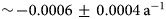
A final example of the utility of the harmonized albedo product is an examination of whether the Dark Zone is progressively darkening over time. Figure 10 shows that the average annual minimum albedo of the Dark Zone during July and August, defined by the albedo threshold α vis-nir < 0.45, has been declining gradually over time (Fig. 10). The darkening rate is ~$-0.0006 \pm 0.0004\, {\rm a}^{-1}$ between 2001 and 2020. However, the darkening is not spatially uniform across the Dark Zone.

Fig. 10. Annual variability of the minimum albedo in July–August recorded within the Dark Zone (2001–20). The aoi is shown in Figure 11. The linear fitting (slope: −0.0006 ± 0.0004, p − value = 0.16) line is also illustrated.

Fig. 11. Time series analysis of the Dark Zone on the GrIS. The cumulative monthly albedo anomalies were calculated using the monthly average albedo of July and August from 2005 to 2020 (a). The occurrence of dark ice shows how frequently an area gets dark in 2005–20 (b). The classification map of occurrences (c) is based on the threshold listed in the top right chart (d). The pie chart (d) summarizes the area comparison of each occurrence class. The Mann–Kendall's tau value of the albedo acquired in July and August 1984–2020 (e) shows the trend in albedo change. The overall occurrence of dark ice including the first stage (1984–2020) is shown in (f). The study area was highlighted on the base map of average albedo (g) in July–August 2015.
Figure 11a shows the spatial cumulative albedo anomalies across the Dark Zone. The region of interest (shadowed area in Fig. 11g) was restricted to the latitude between 63$^\circ$ N and 71$^\circ$
 N, which was adopted from Wientjes and others (Reference Wientjes, van de Wal, Reichart, Sluijs and Oerlemans2011) and Ryan and others (Reference Ryan2018) and adjusted by visual examination of the albedo product. The ice mask was obtained from GIMP (Howat and others, Reference Howat, Negrete and Smith2014) but small glaciers not connected with the GrIS were excluded. Negative trending albedo anomalies denote darkening and are mostly observed in the northern and central Dark Zone, north of $\sim \!66^\circ$
 N. The northeastern edge of the Dark Zone shows a darkening trend with a cumulative albedo anomaly of ~−3. The southern and the most northern parts of the Dark Zone, by contrast, exhibit slight brightening with cumulative albedo anomalies that are slightly positive.
The extent of the Dark Zone is highly variable, both spatially and temporarily (Fig. 8), and hence the occurrence of the dark ice also evolves over time (Figs 11b, c, f). The frequency of dark ice occurrence is calculated by normalizing the number of years with annual albedo minima <0.45 (July–August) to the total number of years with valid observations (number of clear observations >0). This is to exclude the potential data gaps (see the section on narrow to broadband conversion results). The occurrence of dark ice between 2005–20 is higher in the center of the Dark Zone, where ice becomes persistently dark (Fig. 11c), while more than half ($59\percnt$ ) of the surrounding ice areas have a dark frequency <0.5. The Dark Zone is relatively small in the first stage (1984–2004), and the frequency of dark ice (1984–2020) is lower compared to 2004–20 (Fig. 11f). The Mann–Kendall's test is a non-parametric rank correlation test for trend detection (Mann, Reference Mann1945; Kendall, Reference Kendall1975; Morell and Fried, Reference Morell and Fried2009), and is commonly used in time series analysis of geospatial data. A positive tau value corresponds to an increasing trend over time and a negative tau value corresponds to a decreasing trend. Figure 11e shows a darkening trend in the periphery of the Dark Zone and is close to neutral in the center. However the trends are not statistically significant (p < 0.05) for the majority of pixels, perhaps due to imbalanced data density in our harmonized dataset. This emphasizes the importance of temporal resolution of the utilized dataset in time series analysis.
Discussion
We have produced a harmonized time series of albedo variations on the GrIS from 1984 to 2020. The data harmonization was achieved by cross calibrating L4–L7 and S2 spectral bands to L8 SR bands using band to band regression coefficients. The RMA regression model was chosen for the cross-sensor transformation functions because it was computationally less intensive, yet still sufficient for harmonizing the Landsat and S2 image collections. The narrow to broadband conversion algorithm was built by regression analysis of harmonized satellite data and in situ albedo measurements from PROMICE AWS. The conversion algorithm was built with VIS-NIR bands (Eqn (5)) and outperforms other models and reference albedo products. The time series of derived albedo enables us to investigate albedo dynamics at both point and regional scales.
Data density
One of the issues that limits quantitative analysis of the variations is the non-uniform availability of clear observations, which results in gaps in the time series (Zhang and others, Reference Zhang, Shang, Rittenhouse, Witharana and Zhu2011). For example, the Landsat dataset is affected by sensor saturation, cloud masking (Ernst and others, Reference Ernst, Lymburner and Sixsmith2018; Zhu, Reference Zhu2019) and the scan line error on L7 ETM+ (Maxwell and others, Reference Maxwell, Schmidt and Storey2007; Chen and others, Reference Chen, Zhu, Vogelmann, Gao and Jin2011; Zhu and others, Reference Zhu, Woodcock, Holden and Yang2015b), which may confound simple band to band regression and the time series analysis of albedo. One way of dealing with time series data with irregular data density is to aggregate a longer time span of data for periods with fewer available images.
The improved radiometric resolution of L8 OLI and Landsat 9 (L9) reduces the error caused by saturation over snow (Wang and others, Reference Wang2016; Masek and others, Reference Masek2020). However, the saturation bitmask of Landsat and S2 still masks out large areas of inland Greenland where albedo is high (Fig. 11g).
The temporal coverage of L8 and S2 substantially improves the monitoring ability and enables us to capture the seasonal evolution of albedo. The temporal resolution of Landsat and S2 when combined is $> \!100\, {\rm a}^{-1}$ . Recently released Landsat Collection 2 data are used, and there is also scope for the incorporation of L9 data in future. All Landsat data acquired from 2022 will be processed and available only in Collection 2 (Masek and others, Reference Masek2020).
Data harmonization
Harmonization of the surface reflectance products of Landsat Collection 2 and S2 is achieved by using statistical sensor transformation functions optimized for ice/snow. This allows us to generate a consistent long time series of satellite observations that can be applied to a wide range of applications in glaciological remote sensing. The processing procedures are mostly adapted from Roy and others (Reference Roy2016a) and adjustments were made to account for the high spatial and temporal variability of snow- and ice-covered surfaces.
The band to band regression (Figs 3, 4) is more scattered in comparison to the analysis of mid-latitude areas (Roy and others, Reference Roy2016a). The time window of pairing the reference SR band ($\alpha _{\rm band}^{\rm SRref}$ ) and the matched target SR data ($\alpha _{\rm band}^{\rm SR}$
 ) is 24 h. The ice surface is highly dynamic during the melt season and the paired pixel values are more dispersed due to the rapid changes within the 1 d time window. The cross-sensor comparison of SR values reveals that L8 is generally higher than L7 and S2 across all bands. The spectral conversion function that harmonizes the SWIR1 band from the L4–L7 to the L8 has a lower R value (0.59). Therefore, special attention needs to be given to the harmonization of Landsat TM/ETM+ SWIR1 dataset.
The regression fits would have zero intercepts and all data points would reside on the 1:1 reference line if the sensors were identical and images were acquired at the same time (Roy and others, Reference Roy2016a). However, sensors do not make simultaneous measurements and the difference between acquisition time can be up to 24 h. Hence, the band to band regressions are not forced through 0 due to the cross-sensor differences.
Sensor saturation still persists on the VIS-NIR bands in the pixel-by-pixel analysis of Landsat data after the saturation mask is applied (Fig. 3). The bitmask that comes with Landsat's QA_RADSAT is insufficient to fully exclude the influence of radiometric saturation, but it is as adequate because the saturated pixels at higher SR values (>0.8 or >0.9) was just a small fraction of the total usable data. The impact of sensor saturation is minimized in the comparison of S2 and L8 (Fig. 4) due to the similarity in their absolute radiometric resolution (Pahlevan and others, Reference Pahlevan, Chittimalli, Balasubramanian and Vellucci2018).
Narrow to broadband conversion
The narrow to broadband conversion formulas were built from the relations between the satellite pixel values and in situ albedo measurements. The predicted albedo from these algorithms (Eqns (4–6)) were compared to the MODIS albedo product (MOD10A1.006) and a broadband estimation algorithm from the literature (Eqn (3)). The validation with in situ measurement is good, with R 2 > 0.68 for total and VIS-NIR band models (Eqns (4)–(5)). The optimal narrow to broadband conversion algorithm took both the model performance and data density issues into account. The algorithm that utilizes the VIS-NIR bands alone (Eqn (5)) was chosen since it allows the utilization of more of the available datasets (Fig. 5) (Ernst and others, Reference Ernst, Lymburner and Sixsmith2018) without compromising the reliability of the derived albedo. A key benefit is that more clear observations have become available (Ernst and others, Reference Ernst, Lymburner and Sixsmith2018) and are not lost due to data saturation on the SWIR1/2 bands.
The spatial window size for extracting the time series dataset at the point scale is of vital importance (Pahlevan and others, Reference Pahlevan, Chittimalli, Balasubramanian and Vellucci2018). It has a direct impact on the capacity of satellite data to reveal local scale surface processes. The higher spatial resolution of Landsat and S2 helps overcome the overestimation of albedo from satellite images with coarser resolution, for example, the overestimation of albedo below 0.4 by the MODIS albedo product (Fig. 5). A 90 m spatial window (equivalent to 3 by 3 Landsat pixels or 9 by 9 S2 pixels in the VIS-NIR bands) was used to extract the pixel values for generating the point scale albedo. We note that seasonal analysis may require a change in the window size as the homogeneity of ice surface albedo varies significantly during the melt season.
Uncertainties in the albedo validation may arise from the groundtruth observations. The PROMICE AWS albedo measurements were used as ‘absolute’ groundtruth data in training the narrow to broadband conversion algorithm and the albedo validation. The mismatch between the spatial resolution of the satellite imagery and the footprint of the local AWS sensor can affect the validation of the albedo product (Stroeve and others, Reference Stroeve, Box and Haran2006; Ryan and others, Reference Ryan2017). How representative the ice surface near the AWS is would also affect the performance of the albedo product (Fig. 7).
Time series analysis of albedo dynamics
The evolution of the maximum extent of the Dark Zone on the GrIS has undergone three different stages. On average, the maximum area of the Dark Zone during the third stage (2008–20) was $\sim \!280\percnt$ larger compared to the first stage (1984–2004). The second transitional stage coincides with a period when the cumulative surface mass balance (SMB) of the GrIS changed from being in a state of balance to increasingly negative, driven by oceanic and atmospheric warming (Shepherd and others, Reference Shepherd2012, Reference Shepherd2020). However, the subsequent variations in the SMB are not matched by variations in the extent of the Dark Zone. Instead, the maximum extent of the Dark Zone has remained relatively stable since the last expansion in 2005–07. A clear trend in the spatial coverage was not found in the inter-annual variations after the expansion, even though the mass loss rate of GrIS peaks in 2012 and has declined since (Shepherd and others, Reference Shepherd2020).
There have been dramatic inter-annual variations in the extent and persistence of the Dark Zone during the past two decades, which can be seen in MODIS albedo products (Shimada and others, Reference Shimada, Takeuchi and Aoki2016; Tedstone and others, Reference Tedstone2017). The Dark Zone area estimated from MODIS expands during 2007, 2010, 2011, 2012, 2014 and 2016 (Tedstone and others, Reference Tedstone2017). This is in good agreement with our findings (Fig. 8), with only one exception in 2011. The minimum area of the Dark Zone in the third stage occurred in 2015 (Fig. 8), and was linked with delayed exposure of bare ice due to the increased snowfall events and mass accumulation before the onset of the melt season (Tedstone and others, Reference Tedstone2017). However, the definition of the Dark Zone using a single annual minimum albedo threshold is sensitive to the frequency of satellite observations. The revisiting time of Landsat is 16 d (8 d with two Landsat satellites) may not be able to capture the short-term (<8 or <16 d of Landsat's revisiting time) darkening event, whereas the combination of Landsat and S2 has a higher temporal resolution (3–5 d). The increased frequency of data collection resulted in the Dark Zone apparently expanding by ~5000 km2 larger in comparison with the Landsat alone estimate. The optimal Dark Zone definition likewise must vary depending on the temporal and spatial resolution of the available data. Therefore, a single canonical value is likely less appropriate than case-use specific definitions. The threshold we applied is a compromise between the empirical albedo value from the literature and the imbalanced data density of available satellite imagery.
The surface ice in the Dark Zone is darkening on average at a rate of $\sim \! -0.006$ decade−1. He and others (Reference He2013) reported an albedo decline at a rate of $-0.028\pm 0.008$
 decade−1 but this rate of decline is for the entire GrIS. The decline in albedo is higher because areas where ablation zone is annually expanding are included, so capturing the large decline in albedo when the mean summer ice surface is transiting from snow to bare ice. Our lower rate is derived only from the albedo of bare ice in the Dark Zone, defined with an upper threshold albedo of 0.45, and is the average of the annual minimum albedo of all the dark ice pixels.
The observed albedo trends vary geographically across the Dark Zone. Overall the northeastern and central Dark Zone showed a negative trend (cumulative albedo anomaly <−3), compared to the southern region, where there is at best a slight increase (cumulative albedo anomaly >0) (Figs 9, 11). The darkening of the bare ice surfaces on the GrIS is caused by changes to the ice surface architecture and the presence of light absorbing impurities (LAIs) consisting of mineral dust, and pigmented snow and glacial ice algal cells (Stibal and others, Reference Stibal2017; Williamson and others, Reference Williamson2020; McCutcheon and others, Reference McCutcheon2021). Ryan and others (Reference Ryan2018) demonstrated that these types of LAIs could account for 73% of the spatial variability of surface albedo in the Dark Zone. The lowering of albedo due to the increased bare ice area driven by the enhanced melt is more significant in the snow-covered regions at higher elevations on the GrIS. Interplay between these factors may explain the variations in albedo dynamics observed along the Western coast.
Future work
The harmonized Landsat and S2 dataset makes it possible to analyze time series of albedo at high (30 m) resolution, allowing research on, for example, topographical controls on albedo and feedback with local melt rates. It also enables us to obtain albedo data at sites where no in situ measurements are available. Our dataset can be used to analyze long spatiotemporal trends in albedo in glacier ablation zones, especially Greenland's Dark Zone, because the inter-sensor differences are accounted for by our calibrations. This work provides the community with the first medium resolution albedo product optimized for the ablating parts of the western part of the GrIS. The narrow to broadband conversion algorithm for predicting albedo is not yet validated in other areas. Future work could extend the analysis and validate the harmonized albedo product in glaciated areas outside Greenland.
The potential impact of L7's orbit drift after its final ‘inclination’ maneuver, to minimize the impact of declining fuel on board, was not considered. The drift of orbit results in an earlier acquisition time of imagery. Qiu and others (Reference Qiu, Zhu, Shang and Crawford2021) determined that images collected until 2020 are still reliable but L7 may gradually lose its science capability from 2021 onward. Future data harmonization of images captured from 2021 until when L7 phased out and replaced by L9 must correct the deviations caused by the continuously earlier acquisition (local revisiting) time of L7. Studies that require accurate absolute radiometric values may also discard L7 data acquired since 2021.
A comparison of cloud mask algorithms found that Sen2Cor performed poorest among selected cloud detection algorithms (Tarrio and others, Reference Tarrio2020). Hence, a better cloud mask should be included in the current workflow in the future.
We took advantage of existing high level SR products, which include cloud and pixel saturation masks. The invalid SR values (>1), after applying the scale and offsets, are discarded as computational artifacts generated during the atmospheric correction (U.S. Geological Survey, 2021c). The invalid data points are mostly found in the high-albedo range where the sensor is sensing over bright objects such as snow. More usable data would be available for monitoring fresh snow-covered areas (α > 0.8) by improving the atmospheric correction.
Snow and ice surfaces have unique BRDF shapes. The differences in solar and view zenith angles between Landsat and S2 demand BRDF modeling (Claverie and others, Reference Claverie2018). Many current albedo remote-sensing products (Claverie and others, Reference Claverie2015; Li and others, Reference Li2018) rely on the MODIS BRDF product (MCD43A1.006). The coarser spatial resolution of MODIS may introduce artifacts in the harmonized Landsat and S2 datasets (Claverie and others, Reference Claverie2018). The c-factor BRDF normalization uses fixed BRDF global coefficients to provide consistent view angle corrections (Roy and others, Reference Roy2016b). It has been implemented and evaluated in Landsat and S2 products (Roy and others, Reference Roy2017; Claverie and others, Reference Claverie2018) and was suggested by Qiu and others (Reference Qiu, Zhu, Shang and Crawford2021) for correcting the L7 images affected by orbital drift. However, the global coefficients were retrieved over a wide range of land cover types excluding snow/ice-covered areas. Therefore, greater errors might be introduced to Landsat and S2 without BRDF coefficients optimized for snow and ice surfaces. We hope to develop the c-factor BRDF normalization optimized for snow/ice surfaces in future work to address this issue.
Conclusions
A simple, pragmatic and efficient statistical approach was tested and validated to harmonize Landsat surface reflectance (Level-2, Collection 2, Tier 1) and Sentinel 2 Level-2A orthorectified atmospherically corrected surface reflectance products from 1984 to 2020. An RMAlinear regression model was considered as the optimal sensor transformation function to cross calibrate L4–L7 and S2 to L8. The sensor transformation functions may find applications in a wide range of glaciological remote-sensing activities. A narrow to broadband algorithm was derived from the relations between PROMICE AWS albedo measurements and the harmonized satellite data. The predicted albedo from the combination of VIS-NIR bands outperformed other predicted albedo products and the MODIS-derived albedo (MOD10A1.006). The long time series of albedo was reconstructed by applying the optimal narrow to broadband formula to harmonized satellite data. The maximum extent of the Dark Zone increased dramatically during a transition period (2005–07) and stabilized at ~8000 km2 in subsequent years, some 2.8 times the average maximum area from 1984 to 2004. Albedo trends vary geographically across the Dark Zone. The overall darkening rate in the Dark Zone is $\sim \! -0.0006\pm 0.0004\, {\rm a}^{-1}$ in 2001–20. Future research is likely to focus on incorporating more satellite data and validating the albedo product in other areas. This product aids the analysis of small-scale local melt processes and understanding of the processes driving albedo variations.
Data
The source codes for data processing, analysis and an image harmonization tutorial are available at GitHub: https://github.com/fsn1995/Remote-Sensing-of-Albedo (doi: 10.5281/zenodo.7642574). The data harmonization and narrow to broadband conversion discussed in this paper are implemented in a webapp (https://fsn1995.users.earthengine.app/view/albedoinspector, Appendix A Fig. 12).
Acknowledgements
This publication is part of the Deep Purple Project. The project receives funding from the European Research Council (ERC) under the European Union's Horizon 2020 research and innovation program under grant agreement No 856416. DEMs provided by the Polar Geospatial Center under NSF-OPP awards 1043681, 1559691, and 1542736. The authors thank the editor Dr Carleen Reijmer, Dr Nicolas Cullen and the two anonymous referees for their constructive comments. We thank all the contributors to the Google Earth Engine community. We also express our gratitude to Ate H. Jaarsma who helped proofread the manuscript draft and Dr Athanasios Zervas who helped with the server.
Appendix A. Web application: Albedo Viewer
The albedo viewer (Fig. 12) is a Google Earth Engine App (https://fsn1995.users.earthengine.app/view/albedoinspector) that allows users to interactively inspect the time series of albedo by clicking on the map. The basemap is ArcticDEM (Porter and others, Reference Porter2018) and users could load the satellite image of natural color composite and the derived albedo from the time of interest via the drop down button. The time steps of image mosaic can also be adjusted. All maps are masked by the Greenland Mapping Project (GIMP) (Howat and others, Reference Howat, Negrete and Smith2014). Albedo data can also be downloaded as csv for point scale and geotiff for spatial analysis via the app.

Fig. 12. Web application: Albedo Viewer. The web application is an Earth Engine App. It allows users to interactively inspect time series of albedo from the location of interest and load the albedo and the natural color composite satellite image from the time of interest. Basemap is ArcticDEM mosaic (Porter and others, Reference Porter2018) and maps are masked by the Greenland Mapping Project (GIMP) (Howat and others, Reference Howat, Negrete and Smith2014). Landsat 7 images acquired after 2020 are excluded from the analysis due to the orbit drift issue.


 Open access