1. Introduction
Until recently, the dynamics of modern ice sheets were thought to vary substantially only on timescales of centuries to millennia (Reference PatersonPaterson, 1994). Before the mid-1990s, observations of changes in ice-flow speed were limited to a few glaciers, some of which exhibited surge-type behavior (e.g. Reference MockMock, 1966; Reference HigginsHiggins, 1991), providing little evidence to suggest ice discharge from Greenland could change rapidly in a sustained way. This view was consistent with whole ice-sheet models suggesting that the contribution of ice dynamics to the total ice loss over this century will be modest (10–20%) and mass losses will be dominated by surface mass balance (80–90%) (Reference Huybrechts, Gregory, Janssens and WildHuybrechts and others, 2004). The expansion of observational ability over the past decade, particularly in air-and spaceborne remote sensing, has dramatically altered this perspective by revealing major changes in ice-sheet and outlet glacier flow over timescales of days to years (e.g. Reference Howat, Joughin and ScambosHowat and others, 2007; Reference JoughinJoughin and others, 2008a; Reference NettlesNettles and others, 2008). Numerous observations resulting from this improved capability have focused attention on increasing rates of ice flow and ice discharge as important potential contributors to 21st-century sea-level rise (e.g. Reference Rignot and KanagaratnamRignot and Kanagaratnam, 2006; Reference Velicogna and WahrVelicogna and Wahr, 2006).
Since its first application to ice sheets (Reference Goldstein, Engelhardt, Kamb and FrolichGoldstein and others, 1993), interferometric synthetic aperture radar (InSAR), along with optical-image-tracking methods, has rapidly evolved to provide unprecedented capability for measuring glacier velocities over wide areas (e.g. Reference JoughinJoughin and others, 1999b; Reference JoughinJoughin, 2002; Reference Howat, Joughin, Tulaczyk and GogineniHowat and others, 2005; Reference RignotRignot and others, 2008b). The spatial coverage provided by these methods is complemented by the fine temporal (∼15 s) resolution provided by the GPS (Reference Bindschadler, Vornberger, King and PadmanBindschadler and others, 2003; Reference King and AokiKing and Aoki, 2003), which became available over roughly the same period as InSAR. Together these observational methods provide the capability needed to observe variation in ice-sheet and outlet glacier flow at timescales ranging from seconds to years.
One of the first large changes observed in Greenland was the doubling in speed of Jakobshavn Isbræ (also known as Ilulissat Glacier and Sermeq Kujalleq) over the interval when its floating ice tongue thinned rapidly and eventually disintegrated (Reference Thomas, Abdalati, Frederick, Krabill, Manizade and SteffenThomas and others, 2003; Reference Joughin, Abdalati and FahnestockJoughin and others, 2004). Later observations revealed large speed-ups on the two largest east coast glaciers, Helheimgletscher and Kangerdlugssuaq Gletscher, in 2002 and 2004, respectively (Reference Howat, Joughin, Tulaczyk and GogineniHowat and others, 2005; Reference Luckman, Murray, de Lange and HannaLuckman and others, 2006). Comprehensive mapping soon indicated that discharge from Greenland increased by just over 30% from 1996 to 2005 as many of the ice sheet’s outlet glaciers south of 70° N sped up by roughly 50–100% (Reference Rignot and KanagaratnamRignot and Kanagaratnam, 2006). Because Helheimgletscher and Kangerdlugssuaq Gletscher slowed and thinned by tens of meters after their initial speed-up, discharge from these glaciers decreased substantially from peak values just a few years earlier (Reference Howat, Joughin and ScambosHowat and others, 2007). In addition, Helheimgletscher appears to have undergone at least one other period of speed-up and retreat earlier in the 20th century, before thickening and readvancing prior to its recent speed-up (Reference JoughinJoughin and others, 2008b). Along the southeast coast, a study of 32 glaciers indicates a complicated pattern of speed-up and slowdown over a 6 year period (Reference Howat, Joughin, Fahnestock, Smith and ScambosHowat and others, 2008b), consistent with strong thinning in the region (Reference KrabillKrabill and others, 2004; Reference Howat, Smith, Joughin and ScambosHowat and others, 2008a).
Observations from the 1980s of negligible seasonal change on Jakobshavn Isbræ suggested there was little seasonal variation of outlet glacier flow in general (Reference Echelmeyer and HarrisonEchelmeyer and Harrison, 1990). Subsequent observations, however, have revealed that there is substantial seasonal modulation of the flow of the ice sheet that feeds these outlets. Year-round velocities measured at Swiss Camp first revealed that the ice-sheet margin responds seasonally to surface melt, with summer surface speed enhanced by up to 28% near the equilibrium line (Reference Zwally, Abdalati, Herring, Larson, Saba and SteffenZwally and others, 2002), despite roughly kilometer-thick ice separating the melting surface from the bed. Several theoretical results suggested that conduits to the bed could be established if sufficient water was available for hydrofracturing (Reference WeertmanWeertman, 1973; Reference Alley, Dupont, Parizek and AnandakrishnanAlley and others, 2005; Reference Van der VeenVan der Veen, 2007). This theory was confirmed by observations of supraglacial-lake drainage that indicated that water can indeed breach ice >1 km thick through hydrofracture, and that these connections evolve into moulins that persist for the remainder of the melt season (Reference DasDas and others, 2008). The delivery of surface melt to the bed yields a spatial pattern of relatively uniform summer speed-up (50%) over much of the bare-ice zone when averaged over the 24 day interval of RADARSAT InSAR observations (Reference Joughin, Das, King, Smith, Howat and MoonJoughin and others, 2008c). In addition, larger (>100%) short-term (days) speed-ups that correlated with periods of increased melt have been recorded at several GPS sites on the ice sheet (Reference Joughin, Das, King, Smith, Howat and MoonJoughin and others, 2008c; Reference Van de WalVan de Wal and others, 2008; Reference Shepherd, Hubbard, Nienow, McMillan and JoughinShepherd and others, 2009).
Measured seasonal speed-ups (50–100 m a−1) attributable to surface melt on the slow-moving (∼100 m a−) ice sheet have nearly the same absolute magnitude on the fast-moving (>500 m a−1) outlet glaciers, contributing only a small amount to total annual discharge (Reference Joughin, Das, King, Smith, Howat and MoonJoughin and others, 2008c). Substantial seasonal variations on Jakobshavn Isbræ following the loss of a perennial ice tongue appear to be related to advance and retreat of a seasonal ice tongue, potentially controlled by sea ice within the fjord (Reference JoughinJoughin and others, 2008a). Furthermore, many glaciers sped up and/or sustained enhanced speeds during the winter. Thus, the influence of seasonal melt does not appear to contribute substantially to the long-term speed-ups observed on many outlet glaciers, a conclusion also supported by model-based results (Reference Nick, Vieli, Howat and JoughinNick and others, 2009).
Many of the observations just described were made when the Intergovernmental Panel on Climate Change (IPCC) was finishing its Fourth Assessment (Reference SolomonSolomon and others, 2007). The observed changes were rapid, large, and well beyond what could be predicted by the continental-scale ice-sheet models used to make the IPCC sea-level assessments. These changes revealed large gaps in our understanding of how the Greenland ice sheet and its outlet glaciers respond to climate change, leading the IPCC to conclude that changes in ice dynamics may cause large contributions to sea level for which we can derive no upper bound based on present knowledge (Reference SolomonSolomon and others, 2007). Thus, a major challenge for current ice-sheet research is to fill this knowledge gap. Since the observational history is so short relative to glaciological time-scales, it will require years, if not decades, to build an observational record sufficient to constrain prognostic ice-sheet models.
As part of this ongoing observation effort, we have begun to map Greenland ice flow in a systematic fashion. In this paper, we describe results from two comprehensive mappings of ice-sheet flow for the winters of 2000/01 and 2005/06, limited only by gaps in satellite coverage and by InSAR viability in regions with high accumulation rates. Previous efforts have focused on coastal glaciers, with an emphasis on measuring ice discharge (Reference Rignot and KanagaratnamRignot and Kanagaratnam, 2006). Instead we focus on the spatial patterns of variability, and their implications for ice dynamics, as revealed by these two ‘snapshots’ of ice-sheet flow. By providing a general overview of change over this time period, we can guide more focused studies of specific changes. We begin by summarizing the methods used to generate the velocity maps. We then present the data for different areas of the ice sheet and conclude with analysis and discussion of the results.
2. Data and Methods
2.1. Data
In late 2000 and early 2001, during the RADARSAT-1 Modified Antarctic Mapping Mission, the Canadian Space Agency (CSA) acquired nearly complete coverage of Greenland with multiple passes suitable for InSAR (3 September 2000 to 24 January 2001). After the early observations of rapid change in Greenland described above, NASA requested further Greenland coverage. The first set of these acquisitions occurred in the winter of 2005/06 (13 December 2005 to 20 April 2006) when most of the ice sheet was imaged four consecutive times to produce three InSAR pairs. Similar mappings by RADARSAT (not described here) occurred annually through to the winter of 2008/09. While providing nearly complete coverage, both of these datasets have gaps in southern Greenland where the acquisition priority for other modes and locations was higher. We acquired and processed all of the available RADARSAT data from these two time periods to produce two velocity and synthetic aperture radar (SAR) amplitude image mosaics. Results examining outlet-glacier terminus retreat using the SAR image mosaics are described by Reference Moon and JoughinMoon and Joughin (2008). Here we describe the results from the velocity mapping.
2.2. Processing
To process the data, we used the integrated set of SAR, speckle-tracking and interferometric algorithms described by Reference JoughinJoughin (2002). All the data were acquired along descending orbits (i.e. with the satellite moving from northeast to southwest across Greenland), so there were no opportunities to derive velocities using only interferometric phase from crossing orbits (Reference Joughin, Kwok and FahnestockJoughin and others, 1998). Instead, our results are derived entirely from speckle tracking over much of the fast-moving ice (Reference Gray, Mattar, Vachon and SteinGray and others, 1998; Reference Michel and RignotMichel and Rignot, 1999). For many of the slower regions in the interior, we used the interferometric phase for displacements in the range (cross-track) direction, and speckle-tracked offsets in the azimuth (along-track) direction.
With either speckle tracking or interferometric phase, the satellite orbits are too poorly known to determine the surface velocity without additional control. As a result, we performed a least-squares fit to solve for orbit-related geometric parameters (e.g. the baselines between satellite positions) based on several dozen or more control points of known elevation and velocity for each image pair. In coastal areas, we used stationary areas on rock as control points. On the slow-moving ridges in the interior, we used balance velocities to provide control (Reference Joughin, Fahnestock, Ekholm and KwokJoughin and others, 1997). To ensure that absolute errors from these control points were small, we used only balance velocities from regions with speeds less than 5 m a−1.Finally, in those areas along the 2000 m contour, where changes in velocity are expected to be small (e.g. excluding the area above Jakobshavn), we used GPS points collected along the 2000 m contour from 1993 to 1997 (Reference ThomasThomas and others, 2000).
2.3. Sources of error
The use of balance, rather than measured velocities, and GPS velocities collected at times different than the SAR data, may have introduced some degree of error in our estimates. The error in ice-surface velocity resulting from this assumption, however, is likely to be much smaller than if these on-ice control points were omitted. Even if we could achieve the ideal situation where our control points were all measured with GPS at the same time as the SAR data collection, other sources of error would make it difficult to detect change in velocity in the interior regions, where any such change is expected to be small (<10 m a−1). In these slow-moving, interior regions, we do not assign any significance to differences in the velocity field. Along the ice margin (e.g. below about the 2000 m contour), where points on bedrock provide most of the control, control-related errors in flow speed are small (<10 m a−1) relative to variations in ice-flow speed (10 m a−1).
There are several other sources of error in addition to those related to control points. One major source of inaccuracy is error introduced during the matching procedure used to determine the speckle-tracked offsets, which are determined by the degree of correlation between images. These errors are estimated from the image statistics and are included in our formal error estimates (Reference JoughinJoughin, 2002). Height errors in the digital elevation model (DEM) used for topographic correction in the processing can cause velocity errors (Reference Bamber, Baldwin and GogineniBamber and others, 2003), but their effect is usually small relative to the large displacements observed over the 24 day period between images. Some small degree of such error is visible on the rocky areas because DEM-induced errors are much larger over rough terrain. The DEM also introduces errors in the velocity estimates through errors in surface slope, which yields absolute errors of up to about 3% of speed (Reference JoughinJoughin, 2002). Since our two datasets were acquired from nearly identical imaging geometries, however, these errors nearly cancel when evaluating changes in velocity.
Ionospheric variability causes errors in the azimuth component of the speckle-tracked displacement fields (Reference Gray, Mattar and SofkoGray and others, 2000). This yields a distinctive ‘streaked’ pattern of noise in the velocity field with magnitudes of up to several tens of m a−1. These are spatially variable, making it difficult to derive quantitative estimates of their magnitudes. The distinctive noise pattern, however, often makes these errors visually identifiable so they can be accounted for in the interpretation of the data.
3. Results
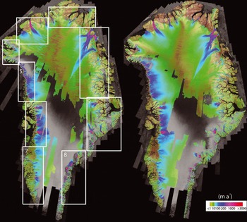
Figure 1 shows the velocity measurements we generated for 2000/01 and 2005/06. A subset of the 2000/01 RADARSAT data was also processed by Reference Rignot and KanagaratnamRignot and Kanagaratnam (2006) at coastal locations, but their 2005 dataset was acquired during the winter prior to our 2005/06 data. As noted above, there are gaps in coverage near the southern end of the ice sheet. Other gaps are the result of poor coherence between images, typically in areas with high snowfall, such as in the southeast. The 2000/01 data were collected near the solar maximum (Reference Richardson, Cliver and CaneRichardson and others, 2001) when the level of auroral-zone ionospheric disturbances was higher, which yields the much larger ‘streak’ errors visible in the 2000/01 velocity map (Reference Gray, Mattar and SofkoGray and others, 2000), particularly in the northwest near the North Magnetic Pole. In addition, a smaller volume of data was collected in 2000/01, yielding less noise reduction through averaging of results from multiple image pairs. To provide a greater level of detail, in the following subsections we present velocity maps for nine regions around the margin of the ice sheet (Fig. 1). The figures for each region (Figs 2–10) show the less noisy 2005/06 map and the difference in speed from 2000/01 to 2005/ 06. These figures also show the amount of the terminus advance or retreat (circles) where this change is >100 m on glaciers 2 km or more wide (Reference Moon and JoughinMoon and Joughin, 2008). Changes on a few of the northern floating ice shelves with poorly defined termini (e.g. Nioghalvfjerdsbræ, Zachariae Isstrøm and C.H. Ostenfeld Gletscher) are not shown.

Fig. 1. Flow speed (color) for the winters of 2000/01 (left) and 2005/06 (right) displayed over radar mosaics (©CSA, 2001) for the same periods. Numbered white boxes indicate the locations shown in Figures 2–10.

Fig. 2. Northeast Greenland flow speed for 2005/06 (top) and change in speed from 2000/01 to 2005/06 displayed over a 2000/01 SAR mosaic (grayscale (©CSA, 2001)) (bottom). Speed is indicated by color and white 250 m a−1 contours (v < 1000 m a−1) and black 1000 m a−1 contours (v ≥ 1000 m a−1). Speed differences are shown with color (saturation is reduced where speed-up or slowdown is <20 m a−1) and 100 m a−1 black (speed-up) and white (slowdown) contours. Blue and red dots indicate retreat (red) and advance (blue).

Fig. 3. Northern Greenland flow speed for 2005/06 (left) and change in speed from 2000/01 to 2005/06 displayed over a 2000/01 SAR mosaic (grayscale (©CSA, 2001)) (right). Speed is indicated by color and white 250 m a−1 contours (v <1000 m a−1) and black 1000 m a−1 contours (v ≥ 1000 m a−1). Speed differences are shown with color (saturation is reduced where speed-up or slowdown is <20 m a −1) and 100 m a−1 black (speed-up) and white (slowdown) contours. Blue and red dots indicate retreat (red) and advance (blue).

Fig. 4. Northwest corner of Greenland flow speed for 2005/06 (left) and change in speed from 2000/01 to 2005/06 displayed over a 2000/01 SAR mosaic (grayscale (©CSA, 2001)) (right). Speed is indicated by color and white 250 m a−1 contours (v < 1000 m a−1) and black 1000 m a−1 contours (v ≥ 1000 m a−1). Speed differences are shown with color (saturation is reduced where speed-up or slowdown is <20 m a−1) and 200 m a−1 black (speed-up) and white (slowdown) contours. Blue and red dots indicate retreat (red) and advance (blue).

Fig. 5. Northwest coastal flow speed for 2005/06 (left) and change in speed from 2000/01 to 2005/06 displayed over a 2000/01 SAR mosaic (grayscale (©CSA, 2001)) (right). Speed is indicated by color and white 250 m a−1 contours (v ≥ 1000 m a−1) and black 1000 m a−1 contours (v ≥ 1000 m a−1). Speed differences are shown with color (saturation is reduced where speed-up or slowdown is <20 m a−1) and 250 m a−1 black (speed-up) and white (slowdown) contours. Blue and red dots indicate retreat (red) and advance (blue).

Fig. 6. West Greenland flow speed for 2005/06 (left) and change in speed from 2000/01 to 2005/06 displayed over a 2000/01 SAR mosaic (grayscale (© CSA, 2001)) (right). Speed is indicated by color and white 250 m a−1 contours (v < 1000 m a−1) and black 1000 m a−1 contours (v ≥ 1000 m a−1). Speed differences are shown with color (saturation is reduced where speed-up or slowdown is <20 m a−1) and 500 m a–1 black (speed-up) and white (slowdown) contours. Blue and red dots indicate retreat (red) and advance (blue).

Fig. 7. Southwest coastal flow speed for 2005/06 (left) and change in speed from 2000/01 to 2005/06 displayed over a 2000/01 SAR mosaic (grayscale (©CSA, 2001)) (right). Speed is indicated by color and white 250 m a−1 contours (v < 1000 m a−1) and black 1000 m a−1 contours (v ≥ 1000 m a−1). Speed differences are shown with color (saturation is reduced where speed-up or slowdown is <20 m a−1) and 250 m a−1 black (speed-up) and white (slowdown) contours. Blue and red dots indicate retreat (red) and advance (blue).

Fig. 8. Southeast coastal flow speed for 2005/06 (left) and change in speed from 2000/01 to 2005/06 displayed over a 2000/01 SAR mosaic (grayscale (© CSA, 2001)) (right). Speed is indicated by color and white 250 m a−1 contours (v < 1000 m a−1) and black 1000 m a−1 contours (v ≥ 1000 m a−1). Speed differences are shown with color (saturation is reduced where speed-up or slowdown is <20 m a−1) and 500 m a−1 black (speed-up) and white (slowdown) contours. Blue and red dots indicate retreat (red) and advance (blue).

Fig. 9. Central east Greenland flow speed for 2005/06 (left) and change in speed from 2000/01 to 2005/06 displayed over a 2000/01 SAR mosaic (grayscale (©CSA, 2001)) (right). Speed is indicated by color and white 250 m a−1 contours (v ≥ 1000 m a−1) and black 1000 m a–1 contours (v ≥ 1000 m a−1). Speed differences are shown with color (saturation is reduced where speed-up or slowdown is <20 m a−1) and 500 m a−1 black (speed-up) and white (slowdown) contours. Blue and red dots indicate retreat (red) and advance (blue).

Fig. 10. Northeast Greenland flow speed for 2005/06 (left) and change in speed from 2000/01 to 2005/06 displayed over a 2000/01 SAR mosaic (grayscale (©CSA, 2001)) (right). Speed is indicated by color and white 250 m a−1 contours (v < 1000 m a−1) and black 1000 m a−1 contours (v ≥ 1000 m a−1). Speed differences are shown with color (saturation is reduced where speed-up or slowdown is <20 m a−1) and 100 m a−1 black (speed-up) and white (slowdown) contours. Blue and red dots indicate retreat (red) and advance (blue).
3.1. Northern Greenland
Accumulation rates in northern Greenland are generally smaller than in the south (Reference Ohmura and ReehOhmura and Reeh, 1991), yielding strong image-to-image correlation. This coherence, combined with the high degree of swath overlap as orbits converge near the pole, provides nearly complete coverage of the northern part of the ice sheet, which we have divided into three sub-regions (Figs 2–4).
3.1.1. Northeastern corner
Figure 2 shows the 2005/06 speed (top) for the northeastern corner of Greenland and the change in speed from 2000/01 (bottom). Also shown in this and in subsequent figures is the retreat of the terminus position (Reference Moon and JoughinMoon and Joughin, 2008). Several small land-terminating glaciers and larger marine-terminating outlet glaciers drain this region of the ice sheet. There are also several ice caps, the largest of which is Flade Isblink in the northeast corner of the image.
The Flade Isblink ice cap is drained mainly by two outlets along its western margin (Reference HigginsHiggins, 1991). In 2005/06, the speeds on these glaciers were low, ranging from an almost completely stagnant northern outlet to a slowly flowing (<60 m a−1) southern outlet. In contrast, the earlier 2000/01 speeds ranged from about 200–300 m a−1 to the north to 300–450 m a−1 to the south, producing the large slowdown visible in Figure 2. The 2000/01 speeds appear higher than those of 175 m a−1 (north) and 360 m a−1 (south) given by Reference HigginsHiggins (1991), but direct comparison is difficult since the exact locations of the earlier measurements are not given. Unlike our measurements, which are derived from images collected over a few months, the earlier measurements were made from photographs collected from 1961 to 1978. Thus, if over this period these glaciers flowed at both the high and low speeds similar to those we observe, this variability might yield intermediate values similar to those measured by Reference HigginsHiggins (1991).
Of the glaciers shown in Figure 2, speed-up is greatest on Hagen Bræ. In the 2000/01 data, the speed on this glacier exceeded 200 m a−1 at 40–75 km inland from the grounding line, diminishing to ∼60 m a−1 just above the grounding line located by Reference Rignot, Gogineni, Joughin and KrabillRignot and others (2001). By 2005/06 this region of compressive strain rates had changed to one of extending flow, with the speed exceeding 600 m a−1 in some areas near the grounding line, which is roughly 75 m a−1 greater than average speeds derived from a 30 year collection of aerial photographs through 1978 (Reference HigginsHiggins, 1991). This speed-up is consistent with the relatively steady acceleration observed near the grounding line from 1996 to 2005 (Reference Rignot and KanagaratnamRignot and Kanagaratnam, 2006). While there was a substantial retreat of the calving front between 2000/01 and 2005/06, much of the ice loss appears to have occurred in places where the tongue was relatively thin and unconfined. Over this period, the SAR images show the ice shelf lost what appears to have been a relatively weak contact with a ‘pinning’ point (island in the fjord). The grounding line is located at a bedrock rise and retreated by 390 m from 1992 to 1996 (Reference Rignot, Gogineni, Joughin and KrabillRignot and others, 2001) in an area near where thinning rates of up to 4 m a−1 were measured over a similar period (Reference AbdalatiAbdalati and others, 2001). Thus, loss of resistance from grounded ice, as well as floating ice in contact with pinning points, may have played a significant role in the speed-up.
Both Academy Gletscher and Marie Sophie Gletscher sped up in the period between our observations, with near-terminus velocities on Academy Gletscher increasing from just over 200 to nearly 600 m a−1, during which time the calving fronts of both retreated by several hundred meters. The Academy Gletscher acceleration followed a large slowdown between 1996 and 2000/01 (Reference Rignot and KanagaratnamRignot and Kanagaratnam, 2006). Using a pair of images from the early 1960s collected 1 year apart, Reference HigginsHiggins (1991) estimated a frontal speed (256 m a−1)close in value to our 2000/01 data. His estimated speed for Marie Sophie Gletscher (220 m a−1), however, considerably exceeds our 2005/06 measurements (<100 m a−1).
Although it lost a large but thin and heavily fractured ice shelf in the intervening period (Reference Moon and JoughinMoon and Joughin, 2008), the speed of C.H. Ostenfeld Gletscher did not change between our two measurement epochs. Its peak speed near the front, of just over 800 m a−1, agrees well with earlier measurements of 760–805 m a−1 prior to 1978 and in the 1990s (Reference HigginsHiggins, 1991; Reference Rignot, Gogineni, Joughin and KrabillRignot and others, 2001), exhibiting much more consistency than the other large glaciers in Figure 2.
3.1.2. Central north
Figure 3 shows several large glaciers in central North Greenland. Ryder Gletscher and Petermann Gletscher show little change. The small amount of apparent change on their floating tongues is likely attributable to uncorrected tidally induced errors. The speeds of both glaciers are consistent with earlier InSAR measurements (Reference Joughin, Fahnestock, Kwok, Gogineni and AllenJoughin and others, 1999a; Reference Rignot, Gogineni, Joughin and KrabillRignot and others, 2001). Our Petermann Gletscher speeds, however, are slightly higher (5–10%) than the 1960s–70s values (Reference HigginsHiggins, 1991); the significance of this is difficult to judge given the unknown errors and the lack of precise location information for the earlier measurements. The shelf front of Ryder Gletscher advanced at about the rate of flow, but it is thin (<200 m; Reference HigginsHiggins, 1991) and fractured in this region, so this advance appears to have had little effect on the overall flow. Our Steensby Gletscher data are roughly consistent with earlier data (Reference HigginsHiggins, 1991; Reference Rignot, Gogineni, Joughin and KrabillRignot and others, 2001) but suggest the glacier slowed by 10–15% over much of its length between 2000/01 and 2005/06.
While Humboldt Gletscher is the widest outlet glacier in Greenland, much of its western side flows slowly, with fast flow (200–500 m a−1) concentrated along its eastern edge (Fig. 3). The eastern edge of this fast-flowing region slowed considerably (∼40%) between 2000/01 and 2005/06, but flow sped up (∼20%) along the western edge.
3.1.3. Northwestern corner
Figure 4 shows the glaciers in Greenland’s northwest corner. Morris Jesup Gletscher and several nearby small and relatively slow-flowing glaciers (∼100–300 m a−1) sped up by several tens of m a−1, representing increases of about 40–150% near their respective termini. As noted by Reference Rignot and KanagaratnamRignot and Kanagaratnam (2006), Tracy Gletscher and Heilprin Gletscher sped up by 40% and 20%, respectively. Both of these increases in speed were accompanied by frontal retreat, with Tracy Gletscher retreating by 1.6 km (Reference Moon and JoughinMoon and Joughin, 2008). Although the mean retreat was substantially smaller for Heilprin Gletscher, there was nearly 1.3 km of terminus retreat along the eastern side of the fjord.
For the small glaciers lying between Heilprin Gletscher and Harald Moltke Bræ, there was relatively little change over our study interval. Harald Moltke Bræ, however, has a well-documented history of surge behavior and variation in position of the ice front (Reference Davies and KrinsleyDavies and Krinsley, 1962; Reference MockMock, 1966). Our 2000/01 measurements show this glacier was moving slowly (30–100 m a−1) within about 8 km of its calving front, with an abrupt transition to substantially faster flow upstream (200–300 m a−1). This flow pattern appears similar to that observed for 1996 (Reference Rignot, Gogineni, Joughin and KrabillRignot and others, 2001). The glacier accelerated between 2000/01 and 2004/05 (Reference Rignot and KanagaratnamRignot and Kanagaratnam, 2006), and our 2005/06 data show speeds exceeding 2000 m a−1 near the front. Our ongoing RADARSAT velocity-mapping efforts indicate that by winter 2006/07 (not shown) the front had slowed and returned to speeds similar to those observed in 2000/01.
Figure 4 also shows several glaciers along the far northern extent of Greenland’s west coast, nearly all of which have sped up. The largest of these increases in speed was on Døcker Smith Gletscher, which sped up by >500 m a−1 as its calving front retreated by >4 km. Since our observations cover a 1 year longer period relative to earlier observations from 2000/01 to 2004/05 when no change was reported (Reference Rignot and KanagaratnamRignot and Kanagaratnam, 2006), the retreat and speed-up may have occurred between 2004/05 and 2005/06. While smaller in magnitude than the increase on Døcker Smith Gletscher, many of the speed-ups on the other glaciers in this region exceeded 100 m a−1 and were accompanied by terminus retreats of a few hundred meters.
3.2. Western Greenland
As Figure 1 indicates, the character of glacier termini varies from north to south along the west coast, from fast-flowing, marine-terminating outlet glaciers in the north to mostly land-terminating glaciers or ice sheet in the south. We have broken the west coast up into three sub-regions: the northwest, the area near Jakobshavn Isbræ and the southwest (Figs 5–7).
3.2.1. Northwest coast
Figure 5 shows our measurements along the northwest coast. With higher accumulation rates in this region than in the north (Reference Ohmura and ReehOhmura and Reeh, 1991), the higher discharge volumes yield both greater inland speeds and flow that converges on several fast-flowing (>1000 m a−1) outlet glaciers, bounded by numerous bedrock outcrops. For these glaciers, no significant speed-up was noted between 2000/01 and 2004/05 (Reference Rignot and KanagaratnamRignot and Kanagaratnam, 2006). Subsequent work revealed a 20% speed-up on the north branch of Upernavik Isstrøm by 2006/07 (Reference Rignot, Box, Burgess and HannaRignot and others, 2008a), and this change is clearly apparent in Figure 5, along with several other changes that have not been noted previously.
The largest speed-up to the north of Upernavik Isstrøm is on Alison Glacier, between Hayes Gletscher and Igdlugdlip sermia, where the peak speed approximately doubled as the calving front retreated by 8.7 km (Reference Moon and JoughinMoon and Joughin, 2008). Other glaciers in the area around Hayes Gletscher experienced a minor slowdown. This pattern terminates to the north near Steenstrup Gletscher, the front of which sped up by just over 500 m a−1 (∼20%) as it retreated by 1.5 km. A similar retreat occurred on the glacier just to the north of Steenstrup Gletscher, coincident with a ∼50% increase in speed. Smaller speed-ups occurred on several glaciers to the north of Steenstrup, all of which were accompanied by modest retreats. In the region between Igdlugdlip sermia and Upernavik, any speed-ups were relatively small, and Nunatakavsaup sermia slowed by ∼40%.
3.2.2. Central west coast
Figure 6 shows several large glaciers near Disko Bay where the most prominent change is the more than doubling in speed of Jakobshavn Isbræ (Reference Joughin, Abdalati and FahnestockJoughin and others, 2004, Reference Joughin2008a). There was little change on the two next largest glaciers in the region, Rink Isbræ and Store Gletscher, while several of the smaller glaciers underwent minor speed-ups. Sermeq kujatdleq, Sermeq avangnardleq and Kangilerngata sermia all flowed at substantially lower speeds in 2005/06. On the latter two of these glaciers, a detailed 3 year time series from 2004 to 2007 showed strong variation including both substantial speed-up and slowdown (Reference Joughin, Das, King, Smith, Howat and MoonJoughin and others, 2008c). In particular, Kangilerngata sermia twice varied from nearly stagnant, as in Figure 6, to peaks of about 600 and 1200 m a−1.
3.2.3. Southwest coast
Figure 7 shows the southwest coast of Greenland, much of which consists of land-terminating, slow-moving glaciers and ice sheet punctuated by a few fast tidewater outlets. Our repeat measurements for Narssap sermia show that it doubled its speed to >3000 m a−1 in 2005/06. There was also a speed-up of several hundred m a−1 on Kangiata nunâta sermia. Both of these speed-ups are consistent with earlier trends (Reference Rignot and KanagaratnamRignot and Kanagaratnam, 2006).
There are a few modest speed-ups on land-terminating glaciers in this region, in particular in the area around Russell Glacier. We examined a 3 year time series in this region (Reference JoughinJoughin and others, 2008a) and found a seasonal variation in speed on the lower part of this glacier (roughly the same area where speed-up is visible in Figure 7). In this time series over the course of the winter, the speed increases by roughly 50–100 m a−1 near the margin, following a minimum speed at the end of the melt season. Since the 2000/01 data were acquired on average roughly 3 months earlier than the 2005/06 data, the changes at Russell Glacier and near the termini of some of the other slow-moving glaciers may represent a seasonal effect. This effect does not extend far inland, and other sites near 1000 m elevation show a much more subdued winter speed-up (Reference JoughinJoughin and others, 2008a; Reference Van de WalVan de Wal and others, 2008).
3.3. Eastern Greenland
As on the west coast, we have subdivided the east coast into southern, central and northern sub-regions.
3.3.1. Southeast coast
Figure 8 shows ice flow along the southeast coast of Greenland where, as described above, high accumulation rates make it difficult to measure interior flow speeds. This region of the ice sheet is far steeper than the west coast, with a more abrupt transition near the heads of fjords between the slow ice-sheet flow and fast, channelized outlet glacier flow. Recent increases in speed and the accompanying rapid, dynamic thinning contribute to making this the region of greatest current ice loss from Greenland (Reference Rignot and KanagaratnamRignot and Kanagaratnam, 2006; Reference Velicogna and WahrVelicogna and Wahr, 2006; Reference Howat, Smith, Joughin and ScambosHowat and others, 2008a). Our data (Fig. 8) confirm the previously reported speed-ups of numerous glaciers in this region (Reference Rignot and KanagaratnamRignot and Kanagaratnam, 2006), all of which coincide with retreats of their respective calving fronts (Reference Howat, Smith, Joughin and ScambosHowat and others, 2008a).
3.3.2. Central east coast
Outlet glaciers along the central east coast (Fig. 9) tend to flow through long subglacial valleys that extend through a region where much of the bedrock is at elevations exceeding 2000 m (Reference Bamber, Layberry and GogineniBamber and others, 2001) before terminating in fjords at the coast. The largest speed-up we found in this area was the previously documented speed-up on Kangerdlugssuaq Gletscher (Reference Luckman, Murray, de Lange and HannaLuckman and others, 2006). Also evident is a smaller, but still substantial, speed-up on one of the branches of the glacier immediately to the north of Unartit, as well as increases in speed on several other glaciers. The speed of Dendritgletscher approximately doubled, with speeds exceeding 600 m a−1 near the terminus in 2005/06. There are also a few places where glaciers have slowed, but these changes are nearly all <100 m a−1.
Many of the glaciers in this area are either confirmed or suspected surge-type glaciers (Reference Jiskoot, Murray and LuckmanJiskoot and others, 2003). Sortebræ, which surged between 1992 and 1995 (Reference Murray, Strozzi, Luckman, Pritchard and JiskootMurray and others, 2002), moves at just over 100 m a−1 at its terminus in the 2005/06 map, but is almost completely stagnant several kilometers upstream. This map also shows much of the length of Sortebræ West moving at speeds of 100–200 m a−1, but it stagnates over a distance of about 5–10 km from where it merges with the main branch. The two marine-terminating glaciers immediately to the west of Sortebræ and the one immediately to the east are nearly completely stagnant, despite having some features similar to those of nearby currently active glaciers in the SAR imagery. Several other glaciers in this area where surge-type behavior has been observed or suspected (Reference Jiskoot, Murray and LuckmanJiskoot and others, 2003) have low speeds or are nearly stagnant, indicating that they are in their quiescent phase. Unlike most of the speed-ups that originate near a retreating terminus, just to the east of Kong Christian IV Gletscher a small unlabeled glacier sped up by more than a factor of 10 on its upper extent, suggesting a surge occurred.
3.3.3. Northeast coast
With a few exceptions, most notably Zachariae Isstrøm and Nioghalvfjerdsbræ, most of the glaciers along the northeast coast (Fig. 10) flow at relatively low speeds (<200 m a−1).In addition to the many tidewater glaciers, there are several land-terminating glaciers and some glaciers with mixed terminus conditions (e.g. Wordie Gletscher). Little change is evident near the fronts of most of the smaller glaciers in this region, but there are some apparent (<30 m a−1) speed-ups in the upstream regions of many of these glaciers. While relatively high streak noise makes these changes difficult to observe, these increases are generally limited to the regions of fast flow, suggesting some degree of actual speed-up.
The downstream portion of Storstrømmen surged from 1978 to 1984 and subsequently stagnated at the front, while ice continued to flow in the upper regions (Reference Reeh, Bøggild and OerterReeh and others, 1994; Reference Mohr, Reeh and MadsenMohr and others, 1998). This pattern continues through our period of observation, with continued slowing in the downstream part of the region of active flow, parts of which slowed by >60 m a−1. A similar drop in speed occurred in the still-active (>∼10 m a−1) regions behind the stagnant front of L. Bistrup Bræ (near zero speed), just to the south of Storstrømmen.
No significant change in speed was visible on the inland part of the ‘Northeast Greenland Ice Stream’, which discharges ice through Nioghalvfjerdsbræ, Zachariae Isstrøm and Storstrømmen. For Nioghalvfjerdsbræ (also known as 79 North) there was no significant speed-up, and any change visible on its floating ice shelf can be attributed to tidal effects. On Zachariae Isstrøm, the speed-up of 200 m a−1 near the front is roughly consistent with changes observed from 2000/01 to 2004/05 (Reference Rignot and KanagaratnamRignot and Kanagaratnam, 2006), following the loss of a large part of its well-confined ice shelf. A slowdown occurred on a nearly stranded section of the ice-shelf front as ice from the area upstream was removed, creating a case of reverse buttressing in which ice is removed from behind rather than in front.
4. Analysis and Discussion
Our data, along with the many other results cited above, indicate that there is substantial variability in outlet glacier flow at seasonal to decadal timescales. This variability likely results from a number of causes, including conditions that promote surging and rapid retreat of grounded and floating ice. In this section, we discuss a number of these factors in the context of our observations.
4.1. Speed-up and terminus retreat
The concept of ice-shelf buttressing restraining inland flow is well known (e.g. Reference PatersonPaterson, 1994), and recent events have highlighted the significance of the similar restraint provided by grounded ice near the terminus (Reference Howat, Joughin, Tulaczyk and GogineniHowat and others, 2005; Reference Luckman, Murray, de Lange and HannaLuckman and others, 2006). Whether floating or grounded, rapid removal of ice in contact with rock or till removes resistance at one location that must be shifted to the ice–rock interface at the bed or lateral margins to restore force balance. The nonlinear viscous rheology of ice means that this is accomplished through changes in strain rates, which usually lead to increased extensional flow upstream of the area where resistance was lost.
Consistent with many earlier observations, nearly all of the larger speed-ups we observe coincide with a substantial retreat of the ice front. While the coincident retreat and speed-up events do not prove causality, high-rate GPS and survey data have shown that loss of ice due to calving produces an immediate speed-up (Reference Amundson, Truffer, Lüthi, Fahnestock, West and MotykaAmundson and others, 2008; Reference NettlesNettles and others, 2008). At least for large retreats, the relationship between retreat and speed-up follows a proportionality that would be predicted from ice rheology (Reference Howat, Joughin, Fahnestock, Smith and ScambosHowat and others, 2008b). Our results for the whole ice sheet expand upon the conclusions of previous regional studies (Reference Joughin, Abdalati and FahnestockJoughin and others, 2004; Reference Howat, Joughin, Tulaczyk and GogineniHowat and others, 2005, Reference Howat, Joughin, Fahnestock, Smith and Scambos2008b) to indicate that where speed-up and retreat coincide, the speed-up is largely the result of the loss of resistive stress as the terminus recedes.
There are several exceptions where speed-up and retreat are not coincident. For example, on C.H. Ostenfeld Gletscher (Fig. 2), the large floating ice shelf completely disintegrated from 2000/01 to 2005/06, with no significant increase in speed on the grounded ice. This ice shelf, however, was heavily fractured in 2000/01, in particular along the areas in contact with the fjord walls. Thus, it is likely that the shelf provided negligible resistive stress, producing little or no speed-up when it finally completed its disintegration.
Another exception is Kangilerngata sermia (Fig. 6), which slowed between our observations despite a minor retreat. More detailed time series from 2004 to 2007 indicate that this glacier alternated between periods of almost complete stagnation and periods with speeds of 600–1200 m a−1 (Reference Joughin, Das, King, Smith, Howat and MoonJoughin and others, 2008c). A similar, though less pronounced, variation in speed occurred on nearby Sermeq avangnardleq (Fig. 6). While the timings of these changes do not correlate with any retreat of the front, they might have been caused by thinning-induced changes in flotation near the front. Alternatively, they may represent roughly annual-scale changes in the basal hydrological system.
4.2. Influence of bed geometry
Reference McIntyreMcIntyre (1985) suggested that the transition from ice-sheet to streaming flow in Antarctica largely occurs at along-flow, downward steps in the subglacial topography. In formerly glaciated areas of Greenland and elsewhere, such topographic transitions are visible at heads of exposed fjords. For ice-covered areas, however, such topographic transitions are poorly resolved in maps of basal topography (e.g. Reference Bamber, Layberry and GogineniBamber and others, 2001). Nevertheless, the flow patterns visible in Figures 1–10 support the general notion that most rapid flow begins as sheet flow converges on the upstream end of subglacial channels. Such a pattern is clearly evident for Jakobshavn Isbræ (Fig. 6), where the fastest flow (>1500 m a−1) is concentrated in a well-incised channel whose depth reaches around 1500 m below sea level (Reference Clarke and EchelmeyerClarke and Echelmeyer, 1996), with a broad surrounding area of slower but still rapid (>500 m a−1) convergent flow centered about this channel.
Patterns similar to that of Jakobshavn Isbræ are evident for the glaciers along much of the northwest coast (Figs 1, 5 and 6) where accumulation is large enough to produce relatively rapid sheet flow (>150 m a−1)that converges near the coast as it enters narrow glacial outlets, which often terminate between exposed rock outcrops a few kilometers apart. In the northwest, the extent of this rapid, confined flow suggests that most subglacial troughs may extend inland as well-defined features only about 25–50 km from the current margin. This suggests that retreat of the northwest margin by a few tens of kilometers could cause many outlet glaciers to retreat from their deep fjords to areas where the bed is above sea level (Reference Bamber, Layberry and GogineniBamber and others, 2001), as happened during the Holocene to the majority of glaciers in the southwest. If this occurs, then ice loss due to glacier terminus retreat and dynamic thinning will be topographically limited as glaciers quickly retreat into shallower water or regions above sea level. The current, or even moderately elevated, thinning rates for this region, however, could be sustained for decades or centuries. A similar limiting process may occur in the southeast as glaciers recede inland along their fjords to higher ground. A more detailed mapping of subglacial topography is needed to confirm the extent to which troughs extend under the ice sheet.
While significant changes have occurred in both the northwest and southeast, the changes are much larger in the southeast, particularly in terms of the maximum rates of thinning (Reference KrabillKrabill and others, 2004; Reference Howat, Smith, Joughin and ScambosHowat and others, 2008a; Reference Pritchard, Arthern, Vaughan and EdwardsPritchard and others, 2009). This difference, at least in part, may be due to differing bed geometries. In the northwest, the ice sheet confines much of the rapid flow laterally, with exposed rock only bounding flow near the terminus. With this geometry many northwest glaciers should exhibit smaller maximum thinning rates spread over a wider area following speed-up, since inflow from the sides can help offset thinning on the main glacier trunk. In contrast, southeast glaciers flowing through long, confined fjords should exhibit larger peak thinning rates over a smaller area, because compensating flow can only flow in from upstream. Such a contrast has already been noted between Jakobshavn Isbræ – where there is strong inflow from the sides and spatially extensive thinning – and Kangerdlugssuaq (Fig. 9) and Helheim (Fig. 8) glaciers, which are confined by fjord walls and which thinned at greater rates over smaller areas (Reference Howat, Joughin and ScambosHowat and others, 2007). Thus, an equivalent increase in discharge at the terminus will lead to much larger maximum thinning rates near the termini of southeast glaciers that, at least initially, are limited to the narrow confines of the fjord (e.g. Reference Howat, Smith, Joughin and ScambosHowat and others, 2008a). This may lead to more dramatic changes in discharge over short time periods in the southeast, but may allow mass loss over longer time periods in the northwest.
4.3. Seasonality
Our analysis compares two maps that were acquired ∼3 months apart relative to the seasonal cycle: September– January for the 2000/01 data and December–April for the 2005/06 data. Thus, we need to consider the fact that our measurements may reflect some degree of seasonal variability. As described above, in the southwest (Fig. 7) near where we have a detailed time series from other studies, there is some speed-up along the ice-sheet margin that may be entirely the result of seasonal variation in ice-sheet flow, possibly as subglacial conduits that developed during summer drainage close over the winter.
In Greenland, calving rates often vary seasonally (Reference Sohn, Jezek and van der VeenSohn and others, 1998), with substantially less calving in winter than in summer, allowing at least some calving fronts to advance over the winter. For glaciers where speed is influenced by terminus position, this may reduce late-winter speeds (2005/06) relative to early-winter speeds (2000/01). For example, since the loss of its ice shelf, the speed near the front of Jakobshavn Isbræ (Fig. 6) varies seasonally by roughly 20% (Reference JoughinJoughin and others, 2008a). Thus, in some of the areas where we observe lower speeds, some of the change may result from seasonal variability rather than longer-term change.
4.4. Surge behavior
Surge behavior has been observed previously at many locations in Greenland (Reference MockMock, 1966; Reference Reeh, Bøggild and OerterReeh and others, 1994; Reference Rignot, Gogineni, Joughin and KrabillRignot and others, 2001; Reference Murray, Strozzi, Luckman, Pritchard and JiskootMurray and others, 2002). Our velocity maps include most of these glaciers, capturing some in both their surge and quiescent phases. On the ice cap of Flade Isblink (Fig. 2), our results reveal surge behavior that may not have been recognized previously. On many glaciers where surge behavior was believed likely (Reference Jiskoot, Murray and LuckmanJiskoot and others, 2003), stagnant flow observed in our data as well as European Remote-sensing Satellite (ERS)-derived estimates (Reference Luckman, Murray, Jiskoot, Pritchard and StrozziLuckman and others, 2003) indicate surge glaciers in their quiescent stages.
Reference Murray, Strozzi, Luckman, Jiskoot and ChristakosMurray and others (2003) suggested that at least two processes could produce surges. With the first of these, a surge occurs when an efficient basal hydrological system changes to a less efficient linked-cavity system, producing high basal water pressure and fast flow (Reference KambKamb, 1987). This type of surge, typical of Alaskan surges, tends to terminate abruptly when a more efficient drainage network is reestablished. This type of process was likely responsible for the surge of Sortebræ in East Greenland (Fig. 9) in the 1990s (Reference Murray, Strozzi, Luckman, Pritchard and JiskootMurray and others, 2002) and perhaps the small surge we observe on a nearby glacier (Fig. 9). For the second type, the surge begins when basal water production becomes sufficient to weaken soft sediments, potentially leading to a positive feedback whereby increased motion produces more basal melt and more till weakening (Reference Fowler, Murray and NgFowler and others, 2001). This leads to a more gradual build-up in speed and a more gradual termination, which is characteristic of many of the Svalbard surges (Reference Murray, Strozzi, Luckman, Jiskoot and ChristakosMurray and others, 2003). The surge of Storstrømmen (Fig. 10) from 1978 to 1984 may fall into this latter category (Reference Reeh, Bøggild and OerterReeh and others, 1994).
A characteristic of the quiescent phases of Harald Moltke Bræ (Fig. 4), Storstrømmen and L. Bistrup Bræ (Fig. 10) is that the regions above their respective termini are nearly stagnant, while active flow continues farther upstream, with a relatively sharp gradient between active and stagnant flow. The stagnation may be consistent with the presence of subglacial sediments strengthened by the thermal mechanism just described. For Storstrømmen, the still-active region flows over a ∼300 m bedrock high, before the bed plunges several hundred meters to elevations ∼400 m below sea level (Reference Joughin, Fahnestock, MacAyeal, Bamber and GogineniJoughin and others, 2001). It is at this bedrock step that the along-flow slowdown begins, reaching complete stagnation over the deepest regions where marine sediments may exist. It is interesting to note the similarity in the velocity gradients above the stagnant area on Storstrømmen and the similar pattern on Kamb Ice Stream, West Antarctica (Reference JoughinJoughin and others, 1999b), which likely stagnated as water was withdrawn through freezing or drainage from weak subglacial sediments (Reference Kamb, Alley and BindschadlerKamb, 2001). The stagnant part of L. Bistrup Bræ also lies over this deep region, with similar active regions located upstream over regions of higher bed elevation.
An inversion of velocities on nearby Nioghalvfjerdsbræ and Zachariae Isstrøm (Fig. 10) suggests that the areas of these glaciers that are well below sea level contain subglacial tills similar in strength to the weak sediments found beneath the Ross Ice Streams, West Antarctica (Reference Joughin, Fahnestock, MacAyeal, Bamber and GogineniJoughin and others, 2001). Thus, the surge behavior on Storstrømmen, L. Bistrup Bræ and perhaps Harald Moltke Bræ may be subject to a thermally driven feedback in the regions with subglacial sediments. It is important to note that these are tidewater glaciers, so some of the factors that affect non-surge tidewater glaciers may also play a role in the surge cycle. For example, there was a large open area between the termini of Storstrømmen and L. Bistrup Bræ, which closed and made contact with various pinning points as Storstrømmen advanced during its surge (Reference Reeh, Bøggild and OerterReeh and others, 1994). This additional back-stress may have slowed the glacier and reduced basal melt, which could have strengthened the till and contributed to the termination of the surge.
There is flow variability on some glaciers that does not fit traditional surge patterns but nonetheless may have some features in common with more typical surge behavior. For example, the cycling between stagnant and active periods on Kangilerngata sermia (Fig. 6) is far more rapid (12–18 months) than a typical surge cycle (decades). As another example, Academy Gletscher (Fig. 2) varies its flow on decadal timescales, but rather than reaching stagnation it has only slowed to about 200 m a−1,a speed which suggests sliding is still occurring. While these and similar examples may not represent true surge behavior, an understanding of the controls on such variability is important in its own right and may also further understanding of the processes that lead to surge behavior.
5. Conclusions
We have produced two nearly complete velocity maps for Greenland that are part of an ongoing project that will produce similar maps for future years. Consistent with earlier work by others, these results reveal substantial changes on numerous outlet glaciers. The great majority of these changes have been speed-ups associated with terminus retreat of tidewater outlet glaciers. Both velocity maps reveal that most fast flow (>400 m a−1) is limited to narrow, well-defined trunks of outlet glaciers, presumably at locations determined by the subglacial topography. Likewise, the change maps indicate that the large differences in speed are mainly confined to the same fast-flowing regions. This suggests a strong level of topographic control, and while the bed is poorly mapped in many of these areas, the velocity data suggest such topographic control is limited to areas within a few tens of kilometers of the coast. Thus, while outlet glacier dynamics may produce a large contribution to present ice loss, basal topography may limit such retreat to regions near the coast. If this occurs, further ice-sheet loss would be largely controlled by surface mass balance, as is the case now for much of southwestern Greenland.
While surge activity has been noted in several earlier studies, there are relatively few measurements of velocity throughout these surges. Our measurements reveal changes due to surge activity on a number of glaciers around Greenland. With routine annual mapping of velocity, we are gaining an unprecedented ability to monitor and study surge activity in Greenland. Once the early stages of a surge are detected, the international constellation of satellites can be targeted to produce more frequent coverage of individual surges, which will provide a much-needed dataset for understanding the nature of surge dynamics.
Acknowledgements
The raw SAR data were acquired by the Canadian Space Agency’s RADARSAT spacecraft and are archived at the Alaska Satellite Facility. The data were processed under NASA grants NNG06GE5SG and NNX08AL98A. NASA funded additional analysis by I.J., B.S. and I.H. Comments by two anonymous reviewers and H. Fricker improved the original manuscript.