


1. INTRODUCTION
Recent mass-balance studies have shown that Antarctica is losing mass, primarily as a result of accelerating outlet glaciers in the northern Antarctic Peninsula and Amundsen Sea coast of the West Antarctic Ice Sheet (WAIS) (King and others, Reference King2012; Shepherd and others, Reference Shepherd2012; McMillan and others, Reference McMillan2014; Wuite and others, Reference Wuite2015). By contrast, the East Antarctic Ice Sheet (EAIS) appears to be gaining mass due to a recent increase in annual snowfall in some coastal regions (Shepherd and others, Reference Shepherd2012). Studies of EAIS outlet glaciers draining through the Transantarctic Mountains (TAM) have documented no major mass imbalance, but results remain uncertain due to a lack of accurate observations and direct measurements from many areas (Frezzotti and others, Reference Frezzotti, Tabacco and Zirizzotti2000; Rignot, Reference Rignot2002; Rignot and others, Reference Rignot2008; Wuite and others, Reference Wuite, Jezek, Wu, Farness and Carande2009; Todd and others, Reference Todd, Stone, Conway, Hall and Bromley2010; Stearns, Reference Stearns2011; King and others, Reference King2012). However, the potential for change in the TAM outlet glaciers is illustrated well by the distribution of glacial sediments in surrounding ice-free areas (Bockheim and others, Reference Bockheim, Wilson, Denton, Andersen and Stuiver1989; Storey and others, Reference Storey2010; Joy and others, Reference Joy, Fink, Storey and Atkins2014). The along-flow varying extent of moraines and glacial drift sheets show that the behavior of the glaciers is affected by changes in both the EAIS and the Ross Ice Shelf, the latter of which receives two-thirds of its ice from the WAIS (Mercer, Reference Mercer1968; Bockheim and others, Reference Bockheim, Wilson, Denton, Andersen and Stuiver1989; Denton and others, Reference Denton, Bockheim, Wilson and Leide1989a, Reference Denton, Bockheim, Wilson and Stuiverb; Conway and others, Reference Conway, Hall, Denton, Gades and Waddington1999; Fahnestock and others, Reference Fahnestock, Scambos, Bindschadler and Kvaran2000; Bromley and others, Reference Bromley, Hall, Stone, Conway and Todd2010). As a consequence, the TAM outlet glaciers represent key areas for studying the past and present dynamic behavior of both Antarctic ice sheets.
The TAM outlet glaciers exhibit large variations in ice flow dynamics, with surface velocities ranging between more than 1000 m a−1 for the Byrd and David Glaciers (Humbert and others, Reference Humbert, Greve and Hutter2005; Wuite and others, Reference Wuite, Jezek, Wu, Farness and Carande2009) to <20 m a−1 for the Taylor Glacier (Robinson, Reference Robinson1984; Kavanaugh and others, Reference Kavanaugh, Cuffey, Morse, Conway and Rignot2009). Until now, glaciological studies in the TAM have primarily focused on the faster moving outlet glaciers (surface velocities generally above 300 m a−1), while comparatively little is known about the slower moving glaciers (surface velocities generally between 5 and 300 m a−1). The Darwin–Hatherton glacial system (DHGS) belongs to the group of slow-moving TAM outlet glaciers and drains ice into the Ross Ice Shelf. Glacial sediments found in the ice-free valleys surrounding the DHGS provide evidence of at least five episodes of increased ice extent, the timing of which is currently debated (Bockheim and others, Reference Bockheim, Wilson, Denton, Andersen and Stuiver1989; Storey and others, Reference Storey2010; Joy and others, Reference Joy, Fink, Storey and Atkins2014). Like most TAM outlet glaciers, the dynamic behavior of the DHGS is generally poorly understood due to insufficient knowledge of key parameters such as ice thickness, ice velocity, grounding line location and surface mass balance (SMB) (Anderson and others, Reference Anderson, Hindmarsh and Lawson2004; Stearns, Reference Stearns2011). These data gaps have led to considerable uncertainties in modeling the response of the DHGS to changes in climate and surrounding ice masses (Anderson and others, Reference Anderson, Hindmarsh and Lawson2004), and simple extrapolations of glacial drift elevations have been used to infer the Last Glacial Maximum (LGM) ice thicknesses of the WAIS and EAIS (Bockheim and others, Reference Bockheim, Wilson, Denton, Andersen and Stuiver1989; Denton and Hughes, Reference Denton and Hughes2000; Storey and others, Reference Storey2010; Joy and others, Reference Joy, Fink, Storey and Atkins2014). In order (a) to reduce the uncertainties in estimates of past ice thicknesses, and (b) to clarify existing discrepancies about the ages of the glacial drift sheets, and consequently the LGM extent of the glacial system, additional glaciological investigations of the DHGS are required.
In this paper, we present the findings of an airborne and ground-based radar survey that mapped ice thickness, internal features and basal characteristics of the DHGS. In addition, GPS measurements of ice velocities were carried out at various locations throughout the glacial system. From this dataset we aim to: (i) describe in detail the changes in ice thickness, internal layers, ice base, hydrostatic equilibrium, ice flux and basal melt rate, as the DHGS flows across the grounding zone, (ii) provide the first ice thickness and bed topography maps of the DHGS, (iii) discuss observed differences in ice velocity and ice flux between the Hatherton and Darwin Glaciers, and (iv) assess the current mass balance of the DHGS.
The results presented in this paper on grounding zone characteristics, ice flow behavior and balance state provide new information not only about the DHGS, but also of slower moving EAIS outlet glaciers in general. The findings allow for more accurate modeling of the dynamic behavior of these glaciers to future changes in local and regional forcing. Such models will improve our understanding of the ice flow dynamics of the slower moving components of the Antarctic ice masses, and of the surrounding WAIS and EAIS.
2. THE DHGS
The DHGS (152–161°E, 79.3–80.2°S) consists of two main glaciers; the Darwin Glacier which extends from the EAIS to the Ross Ice Shelf, and the Hatherton Glacier which joins the Darwin Glacier downstream of the Darwin Mountains ~40 km upstream of the DHGS outlet (Fig. 1).
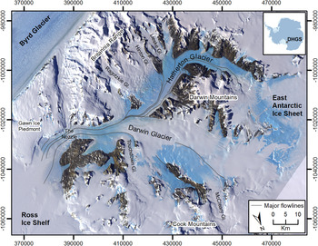
Fig. 1. Regional setting of the DHGS with major glacier flowlines as indicated by bands of sediments visible in blue ice areas. Map based on ASTER images (https://lpdaac.usgs.gov/). Coordinates are in a Polar Stereographic projection with true scale at 71°S.
The glacial system is characterized by the presence of several blue ice areas, prominent medial moraines and large adjacent ice-free valleys covered in glacial sediments. The SMB of the DHGS is largely unknown. However, average daily summer ablation rates of 1 mm d−1 have been measured within the lower Hatherton Glacier blue ice area (Riger-Kusk, Reference Riger-Kusk2011). No direct measurements of accumulation rates exist from within the DHGS catchment, but values are thought to vary between 100 and 150 mm w.e. a−1 on the polar plateau and ~200 mm w.e. a−1 on the Ross Ice Shelf (Bockheim and others, Reference Bockheim, Wilson, Denton, Andersen and Stuiver1989). Several Antarctic-wide maps of SMB cover the region, but due to the lack of direct measurements and relatively low resolutions compared with the topography within the DHGS, none of these models accurately accounts for the observed patchwork of ablation and accumulation areas (Arthern and others, Reference Arthern, Winebrenner and Vaughan2006; van de Berg and others, Reference van de Berg, van den Broeke, Reijmer and van Meijgaard2006; Lenaerts and others, Reference Lenaerts, Van Den Broeke, Scarchilli and Agosta2012a, Reference Lenaerts, van den Broeke, van de Berg, van Meijgaard and Kuipers Munnekeb).
Ice velocities were previously measured along two cross profiles during the 1978–1979 field season, and show that the Hatherton Glacier flows at ~40 m a−1 at the confluence with the Darwin Glacier, while the velocity of the Darwin Glacier increases from ~50 m a−1 at this location to ~120 m a−1 at The Nozzle (Fig. 1, Hughes and Fastook, Reference Hughes and Fastook1981). More recently, Antarctic ice surface velocities have been determined remotely by means of satellite radar interferometry (InSAR, Rignot and others, Reference Rignot, Mouginot and Scheuchl2011b). The resulting map has a spatial resolution of 450 m and shows that the Hatherton Glacier generally moves with velocities of no more than 10 m a−1 and the Darwin Glacier reaches a maximum velocity of ~110 m a−1 at The Nozzle (Rignot and others, Reference Rignot, Mouginot and Scheuchl2011c).
Prior to this work, ice thickness has been measured at several locations along the Darwin Glacier and at two locations on the Hatherton Glacier during airborne radar surveys in the 1970s (Lythe and others, Reference Lythe and Vaughan2000). However, the scarcity of measurements and a 3 km position uncertainty means that these measurements do not allow for the construction of an accurate ice thickness map of the DHGS, and cannot be used to determine the Darwin Glacier grounding line position. The Darwin Glacier grounding line position has previously been determined as part of continental scale studies of the Antarctic coast line (ADD-Consortium, 2000; Scambos and others, Reference Scambos, Haran, Fahnestock, Painter and Bohlander2007; Bindschadler and others, Reference Bindschadler2011), and Humbert and others (Reference Humbert, Greve and Hutter2005) calculated the DHGS ice discharge to 1.03 km3 a−1 from rough approximations of velocity and ice thickness.
Glacial sediments deposited during the last ~1–2 Ma and extending to more than 750 m above the present glacier surface are present in ice-free valleys surrounding the DHGS (Bockheim and others, Reference Bockheim, Wilson, Denton, Andersen and Stuiver1989; Storey and others, Reference Storey2010; Joy and others, Reference Joy, Fink, Storey and Atkins2014). The configuration of the drift-sheet boundaries illustrate that, during episodes of increased ice thickness and extent, the DHGS was thicker toward the Ross Embayment, while only a minor change, if any, appears to have occurred at the threshold to the EAIS (Bockheim and others, Reference Bockheim, Wilson, Denton, Andersen and Stuiver1989). A similar asymmetrical ice thickness change has been documented for other TAM outlet glaciers, and this is thought to reflect episodes of restricted ice drainage caused by an advance of the WAIS grounding line into the Ross Embayment (Bockheim and others, Reference Bockheim, Wilson, Denton, Andersen and Stuiver1989; Denton and others, Reference Denton, Bockheim, Wilson and Stuiver1989b; Conway and others, Reference Conway, Hall, Denton, Gades and Waddington1999; Bromley and others, Reference Bromley, Hall, Stone, Conway and Todd2010). Anderson and others (Reference Anderson, Hindmarsh and Lawson2004) confirmed the linkage between ice thicknesses of the Antarctic ice sheets and the DHGS by matching output from a flow-line model with the Holocene retreat history offered by age determinations of glacial sediments proposed by Bockheim and others (Reference Bockheim, Wilson, Denton, Andersen and Stuiver1989). In addition, Anderson and others (Reference Anderson, Hindmarsh and Lawson2004) provided further insight into the dynamic behavior of the DHGS, suggesting that the Darwin Glacier is entirely wet-based and has a maximum velocity of ~325 m a−1, while the Hatherton Glacier is wet-based in the lower regions only and flows with a maximum velocity of ~15 m a−1. However, as the model of that study relied on insufficient ice velocity measurements and uncertain approximations of ice thickness and grounding line location, direct measurements of these key parameters have the potential to improve model simulation of the present and past behavior of the DHGS and consequently of the EAIS and WAIS.
3. METHODS
Data collection included a ground-based geophysical survey of ice thickness and ice velocity supplemented by an airborne radar survey of ice thickness conducted as part of the ICECAP (Investigating the Cryospheric Evolution of the Central Antarctic Plate) project (Young and others, Reference Young2011). Both surveys were conducted during the 2008–09 field season. The ground-based survey focused on the central flowlines and cross profiles of the Darwin and Hatherton Glaciers and the airborne radar survey collected ice thickness data along the center flowline and upper catchment of the two glaciers (Fig. 2). The two radar surveys complement each other well, with the high-resolution ground-based ground penetrating radar (GPR) system offering a high level of detail and accuracy, and the relatively low-resolution airborne radar system providing strong bed reflections in the deepest and inaccessible regions of the glacial system.
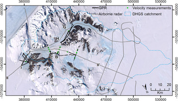
Fig. 2. Field measurements at the DHGS. Black lines show GPR profiles where a basal reflection was detected and gray lines show airborne radar flight paths. Capital letters indicate the location of radar sections and cross profiles referred to in the text. Green circles show the location of successful ice velocity measurements. The dashed blue line show the DHGS catchment which was calculated from the constructed DEM described in Section 3.5. Map based on the Landsat Image Mosaic of Antarctica (LIMA, http://lima.usgs.gov). Coordinates are in a Polar Stereographic projection with true scale at 71°S.
3.1. Ground-based GPR measurements
The ground-based radar survey was conducted using a pulseEKKO PRO GPR system run with a 1000 V transmitter connected to a set of 25 MHz unshielded dipole antennas. For practical reasons, the antennas were oriented parallel to the direction of travel and with an antenna separation of 3 m. In order to minimize the interference of nearby conductors, the antennas were mounted on the skis of a purpose-built plastic sled. The plastic sled was towed 2 m behind an additional wooden sled holding the control unit, GPS and batteries, and this in turn was towed 6 m behind a snowmobile. Individual measurements were automatically stacked 4 times to improve the signal-to-noise ratio of the recorded trace. Radar measurements were recorded in continuous mode at intervals of ~1.5–3 m, depending on travel speed of the snowmobile. Position data were collected for every fifth measurement using a single-frequency Trimble GeoXM GPS receiver.
Processing of the GPR data was carried out in EKKO_View Deluxe and involved, as a minimum, an interpolation of GPS positions to all recorded traces, time zero correction, dewow filtering, bandpass filtering and the application of a gain function (primarily automatic gain control). Further processing was required for the cross profiles which were rubber-banded and migrated (Cassidy, Reference Cassidy and Jol2009), in addition to the more basic processing steps. Interpretations were carried out in the KINGDOM (Seismic Micro-Technology) interpretation software. Although a maximum ice thickness of 1124 m was detected by the GPR just upstream of the Darwin Glacier grounding line, deep basal reflections are generally weak and occasionally fall below the background noise when ice thickness exceeded 700 m.
3.2. Airborne radar measurements
The airborne HiCARS radar system (Peters and others, Reference Peters, Blankenship and Morse2005) recorded stacked traces at 200 Hz, which were further summed coherently to 20 Hz and incoherently averaged to 4 Hz. At the aircraft speed of 90 m s−1, this provided a trace every 20 m along the 650 km survey line (Fig. 2). The data were not further migrated or focused. Position data were recorded using a single-frequency GPS receiver and assigned to each trace. Following processing, clear basal reflections are apparent in all surveyed regions and a maximum ice thickness of 1684 m was recorded on the polar plateau upstream of the Darwin Glacier.
3.3. Radar wave velocity and firn correction
Arrival times of the basal reflections were converted into ice thicknesses using radar velocities of 300 m µs−1 in air (airborne survey only) and 168 m µs−1 for ice, the latter being the radar velocity of pure ice, which is often applied in Antarctic studies where ice temperatures remain largely below the melting point (Frezzotti and others, Reference Frezzotti, Tabacco and Zirizzotti2000; Eisen and others, Reference Eisen, Nixdorf, Wilhelms and Miller2002; Horwath and others, Reference Horwath2006). As the DHGS surface is a patchwork of ablation and accumulation areas, ice thickness measurements were adjusted to account for the presence of a firn layer of variable depth. Values of radar firn correction within the region were calculated from a low-resolution Antarctic-wide model of air layer thickness (van den Broeke and others, Reference van den Broeke, van de Berg and van Meijgaard2008) using the method described by Jenkins and Doake (Reference Jenkins and Doake1991) and Horwath and others (Reference Horwath2006). Given the 55 km spatial resolution of the Antarctic-wide model, blue ice areas were not resolved, and an analysis of firn layer thickness from hyperbolas observed in the GPR data (reflection hyperbola shape analysis) suggests that the Antarctic-wide model underestimates radar firn correction by 4.7 m in accumulation areas. To account for the complex SMB of the DHGS, 4.7 m was added to all grid cells, after which values were interpolated across 5 km (sideways) and 15 km (upstream and downstream) zones surrounding outlines of blue ice areas (0 m firn correction). The size of the interpolated zones was approximated from measured ice flow velocities and rough assumptions on ablation and accumulation rates near blue ice areas (van den Broeke and others, Reference van den Broeke, van de Berg, van Meijgaard and Reijmer2006). This approach produces a map of radar firn correction which incorporates the general trend of the region, as suggested by the Antarctic-wide model, with measurements and observations. The resulting map has a spatial resolution of 50 m and radar firn corrections ranging between 0 m (blue ice areas) and 13.6 m (accumulation area, polar plateau) within the DHGS catchment. Radar firn corrections of between 7 m (Ross Ice Shelf) and 15 m (Vostok Station) are generally observed in Antarctic accumulation areas (Dowdeswell and Evans, Reference Dowdeswell and Evans2004; van den Broeke and others, Reference van den Broeke, van de Berg and van Meijgaard2008) and the range of values within the DHGS appears reasonable.
3.4. Uncertainty of ice thickness measurements
In order to evaluate the uncertainty of the ice thickness measurements, values were compared at 17 locations where survey lines cross. The observed differences in ice thickness at these locations are below 12 m at 14 crossover points, and <3 m in regions where a clear basal reflection was observed (eight crossover points). However, larger uncertainties are observed at three crossover points located close to the margin of the Hatherton Glacier. Here, the ice thickness in migrated GPR cross profiles exceed unmigrated measurements recorded in an along-flow direction by 22–75 m. The observed differences are due to uncorrected side-swipes from subglacial valley walls in the unmigrated longitudinal profiles. The uncertainties observed in along-flow profiles close to the glacier margins are particularly pronounced for the airborne radar due to the larger radar beam, and illustrate the importance of cross profiles and ground-based surveys in mountainous regions such as the DHGS. As the cross profiles were migrated and the majority of unmigrated longitudinal profiles were collected away from the glacier margin, further actions to minimize the influence of subglacial side-swipes on the ice thickness interpretation were not considered necessary.
The combined uncertainty of the ice thickness measurements is primarily a result of uncertainty in radar wave velocity and the interpretation of reflector arrival times. The uncertainty varies across the DHGS, depending on the distance to the glacier margin and the presence of a firn layer. The measurements are generally thought to be accurate to within 10–15 m (an error of <5%), and decreasing to <5 m toward the Darwin Glacier outlet where the firn layer is thin or absent and the basal reflector is strong and smooth.
3.5. Modeling the geometry of the DHGS
A continuous map of surface elevation (50 m spatial resolution) was constructed by combining a 1 km resolution Antarctic-wide DEM presented by Bamber and others (Reference Bamber, Gomez-Dans and Griggs2009) with two higher resolution models which cover only part of the surveyed region. These more detailed models were created by Land Information New Zealand (LINZ, 20 m resolution) and by the SPOT 5 Stereoscopic survey of Polar Ice: Reference Images and Topographies project (SPIRIT, 40 m resolution). The models were merged by using an inverse distance weighting routine and smoothing across 1–2 km wide overlapping regions. The low-resolution Antarctic-wide DEM performs poorly in the steep terrain but well in the flat upper regions, and including the two higher resolution models ensures that the mountainous terrain is preserved in a model, which covers the entire DHGS catchment. The uncertainty of the merged DEM varies according to the topography and the resolution of the original models, and ranges between 1 and 6 m on the ice shelf and polar plateau covered by the Bamber and others (Reference Bamber, Gomez-Dans and Griggs2009) DEM (Griggs and Bamber, Reference Griggs and Bamber2009) to <40 m in the steeper mountainous regions of the DHGS covered by the two higher resolution DEMs.
The construction of the DHGS ice thickness model (50 m spatial resolution) included the following steps: (1) a delineation of rock outcrops (zero ice thickness), (2) a two-dimensional (2D) cubic spline interpolation across data gaps in GPR cross profiles using measurements from the airborne system, the location of the glacier margin and the valley shape as provided by the DEM, (3) linear interpolations of center-line ice thickness between downstream measurements and upstream exposed rocks or measurements for important tributaries not covered by the radar survey, (4) the application of a 3D completely regularized spline interpolation routine (ArcMap) with a search area optimized according to valley shape and the spatial distribution of data points, and (5) smoothing (see Riger-Kusk (Reference Riger-Kusk2011) for additional details). The elevation of the ice base was found by subtracting the ice thickness interpolation from the constructed DEM.
The uncertainty of the glacier bed elevation includes errors in measured ice thickness, surface elevation and most importantly the ice thickness interpolation. The combined uncertainty associated with the model of bed topography increases with distance from measurements and the glacier margin, and is estimated to be no more than ±200 m and generally <±50 m, which is comparable to uncertainties reported in similar studies (Fretwell and others, Reference Fretwell2013; Saintenoy and others, Reference Saintenoy2013).
3.6. Measurements of ice velocity
Ice velocities were measured with a dual-frequency Trimble 4700 GPS at 19 stakes along the center-line of the Hatherton and Darwin Glaciers and along the GPR cross profiles on the Darwin Glacier (Fig. 2). Local base stations were set up on exposed rocks within 20 km of the survey points and the positions of the stakes were usually measured at 3–5 d intervals. The locations of the various base stations were calculated using the nearest two POLENET GPS stations at Butcher Ridge (79.1474°S, 155.8942°E) and Westhaven Nunatak (79.8457°S, 154.2201°E). In addition, the base stations were differentially corrected using the online JPL Automatic Precise Positioning Service (APPS) and survey points were differentially corrected to all base station data within 100 km using the Trimble Geomatics Office software. Five survey points were found to be of poor quality, while the positional uncertainty of the remaining measurements was similar to the instrument specification (±5 mm + 1 ppm of the baseline length) plus inaccuracies associated with positioning the stake (~1 cm). Consequently for a 10 km baseline to our base station, the estimated precision of the measured displacement was ±3.5 cm, which equates to a ~10% error for a typical velocity measurement of 12 cm d−1 (44 m a−1). On the slow-moving Hatherton Glacier, only one of the measurements was successful (Fig. 2). Although this particular measurement was of a high quality, the uncertainty of the method is significant compared with the short distance moved by the stake between measurements.
3.7. Ice flux calculations
Variations in ice flux along the DHGS were calculated from interpolated cross-sectional ice thickness and velocity measurements where possible (cross profiles A, B, C and G, Fig. 2). For cross profiles where velocity measurements were of a poor quality (cross profiles D, E, F and H), the Antarctic-wide dataset of ice surface velocities published by Rignot and others (Reference Rignot, Mouginot and Scheuchl2011b) was applied. A comparison of ice velocities from the two datasets shows that the velocity measurements and the Antarctic-wide dataset compare well. Observed differences are within the uncertainties of the two methods, except for one measurement located between profiles A and B where the grid cell value from the Antarctic-wide map appears unrealistically high compared with the surrounding values. Overall, these good comparisons provide confidence in both datasets.
Continuous velocity profiles were created by fitting either a piecewise cubic or spline interpolation between rocks exposed at the glacier margin (0 m a−1), and point measurements. It was assumed that the velocity vectors were perpendicular to the flux gate in all cases. The additional error introduced by this approach was calculated for all velocity measurements and found to be negligible compared with the uncertainties of the velocity measurements. The total ice flux through each cross profile was subsequently calculated as the sum of flux through 1 m segments using a surface velocity factor (the ratio of column averaged velocity to surface velocity) of 0.87. The value of the surface velocity factor depends primarily on the degree of basal sliding, and a factor of 0.87 implies that some basal sliding occurs along the DHGS. Values ranging from 0.85 to 0.92 have been measured from inland ice masses and toward the Wilkes Land coast (Budd and others, Reference Budd, Jenssen and Radok1971) and a value of 0.87 has previously been applied as an average value in Antarctic studies of ice flux (Budd and Warner, Reference Budd and Warner1996; Fricker and others, Reference Fricker, Warner and Allison2000). A surface velocity factor of 1 was applied for the predominantly floating cross profile E.
Uncertainties associated with the calculated ice flux are highest for profiles C and D where cross-sectional ice thicknesses rely largely on interpolated values, and profiles F, G and H where the uncertainties associated with the velocity data (up to 8 m a−1) are high compared with the speed of the glacier (Rignot and others, Reference Rignot, Mouginot and Scheuchl2011b, Reference Rignot, Mouginot and Scheuchlc). A general uncertainty of <20% for calculated ice flux is estimated by combining the potential errors associated with (1) measurements and cross-sectional interpolations of ice thickness and ice velocity, and (2) the surface velocity factor. The differences between ice flux at profiles A, B and C calculated using velocity measurements and the Antarctic-wide dataset (Rignot and others, Reference Rignot, Mouginot and Scheuchl2011c) are no more than 0.02 km3 a−1, or ~10%, providing further confidence in the presented values of ice flux.
4. RESULTS
4.1. The Darwin Glacier grounding zone
The position of the central Darwin Glacier grounding line was determined from spatial variations in the ice base reflection observed in a GPR profile collected along the center flowline in an upstream direction (Fig. 3a).
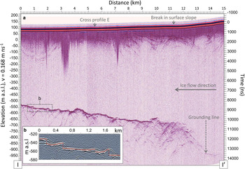
Fig. 3. (a) Unmigrated GPR profile crossing the central Darwin Glacier grounding line (I – I′ transect in Fig. 2), with enlarged sections of (b) the ice base. The profile has been topographically corrected using the Bamber and others (Reference Bamber, Gomez-Dans and Griggs2009) DEM.
Upstream of the central grounding line, which is located at ~13.8 km in Fig. 3a, a weak basal reflection is detected to a depth of 1124 m before falling below the level of the background noise. The ice base reflection becomes indistinct at the grounding line due to an abundance of reflection hyperbolas, indicative of a sudden change in basal topography (Jol, Reference Jol2009). The hyperbolas are interpreted as basal crevasses, which form near grounding lines due to a combination of tidal flexure and shear stresses in this region (Jezek and Bentley, Reference Jezek and Bentley1983; Rist and others, Reference Rist, Sammonds, Oerter and Doake2002; Catania and others, Reference Catania, Hulbe and Conway2010). At the central grounding line, measurements show that the Darwin Glacier is ~1050 m thick and resting on a bed located ~925 m below sea level. Three kilometers downstream, as the basal reflection becomes visible again, a ~250 m decrease in ice thickness has occurred. As the distance from the grounding line increases, the number of hyperbolas decrease, the ice base reflection becomes smoother and stronger, and near horizontal terraces develop (Fig. 3b). The terraces have widths of 100–1000 m and are observed on both the longitudinal GPR profile (Fig. 3b) and cross profile E. Each terrace ends in single-sided hyperbolas, associated with the sudden 5–10 m elevation change observed in the ice base at the terrace walls.
Downstream of the central grounding line, several large cone-shaped features of enhanced reflectivity extend from the surface to a depth of up to 400 m, most noticeably at 3 km in Fig. 3a. These features relate to the reverberation of radar waves in shallow subsurface ponds observed during the fieldwork. Such ponds are well documented elsewhere in low-elevation blue ice areas, where an increased amount of shortwave radiation is absorbed due to the low albedo of blue ice, resulting in melting below the glacier surface (Brandt and Warren, Reference Brandt and Warren1993; Winther and others, Reference Winther, Elverhøy, Bøggild, Sand and Liston1996; Rasmus, Reference Rasmus2009).
The central Darwin Glacier grounding line is located ~2.5 km upstream of a noticeable change in surface slope (Fig. 3a). Such breaks in surface slope have often been used as a proxy for the grounding line location (Scambos and others, Reference Scambos, Haran, Fahnestock, Painter and Bohlander2007; Brunt and others, Reference Brunt, Fricker, Padman, Scambos and O'Neel2010; Bindschadler and others, Reference Bindschadler2011) while the grounding line ice thickness is often inferred from assumptions of hydrostatic equilibrium at this location (Rignot and Jacobs, Reference Rignot and Jacobs2002; Rignot and Thomas, Reference Rignot and Thomas2002). Where ice thickness measurements exist, these can be compared to the calculated ice thickness to investigate variations from hydrostatic equilibrium across the grounding zone. In order to test the assumption of hydrostatic equilibrium at this location, the ice thickness (Z) was calculated along the airborne radar profile using the following equation for a freely floating ice shelf
 $$Z = \displaystyle{{\rho _{\rm w}} \over {\rho _{\rm w} - \rho _{\rm i}}} h - \displaystyle{{\rho _{\rm i}} \over {\rho _{\rm w} - \rho _{\rm i}}} \delta. $$
Where ρ w and ρ i are the densities of sea water (1029 kg m−3) and ice (917 kg m−3), respectively, h is the surface height and δ is the thickness of an air layer calculated from the firn layer correction (Horwath and others, Reference Horwath2006).
The calculated and measured ice base elevation compare well between the beginning of the radar profile and ~2.5 km downstream of the inferred central grounding line (Fig. 4). Any observed discrepancies in this region mimic the inferred rate of changes in firn layer thickness downstream of the blue ice area and consequently appear to reflect uncertainties in firn layer thickness as opposed to actual deviations from hydrostatic equilibrium. Further upstream, the difference between measured and calculated ice base increases rapidly in response to increased surface elevations and therefore the calculated ice thickness. Ice thickness is well above the floatation level upstream of the inferred central grounding, and the deviation from hydrostatic equilibrium confirms that the Darwin Glacier is grounded at this location. It is also evident that the ice is elevated above hydrostatic equilibrium until ~2.5 km downstream of the central grounding line, where hydrostatic equilibrium is achieved.
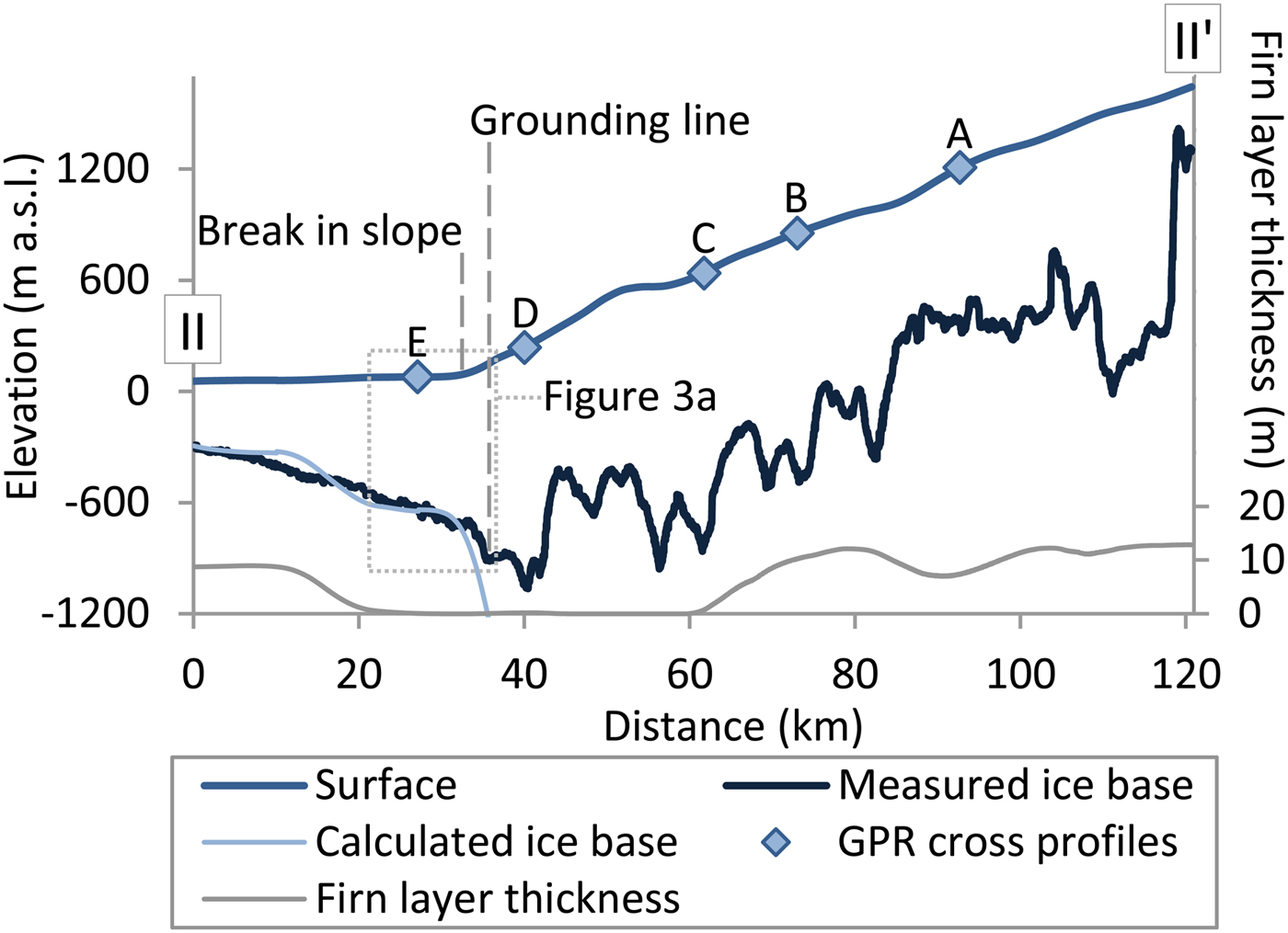
Fig. 4. Surface elevation, firn layer thickness and measured and calculated ice base along a longitudinal airborne radar profile of the Darwin Glacier (II – II′ transect in Fig. 2).
4.2. Ice thickness and bed topography
Considerable spatial variations in ice thickness and bed topography occur along the central part of the Darwin Glacier, with ice thicknesses varying between a minimum of 635 m and a maximum of 1500 m downstream of cross profiles A and C, respectively (Fig. 4). A clear longitudinal change in basal characteristics can be seen in the radar data between the relatively smooth floating ice and highly undulating grounded ice, providing further support to the inferred location of the Darwin Glacier grounding line (Fig. 4). The Darwin Glacier is grounded well below sea level for more than 40 km upstream of the grounding line and several large troughs and ridges exist underneath the glacier. Rapid changes occur at the threshold to the polar plateau, where the bed elevation can be seen increasing 1000 m over a distance of <2 km (at 120 km distance in Fig. 4). At this particular location, ice thickness measurements from airborne cross profiles (Fig. 2) show that the longitudinal profile does not capture the Darwin Glacier center flowline and that ice flows through a deeply carved subglacial canyon located further southwest.
A prominent downstream change in valley shape occurs for the Darwin Glacier as it merges with multiple tributary glaciers before flowing into the Ross Ice Shelf (Fig. 5, profiles A, B, C, D and E). The uppermost Darwin Glacier cross profile A has a wide and somewhat irregular bed, while further downstream, profiles B and C display several prominent glacier benches and a central trough. As the glacier narrows toward the grounding line (located between profiles D and E), the widths of the benches reduce and the cross-sectional area decreases to a minimum at profile D. A large change in glacier geometry occurs between cross profiles D and E, which are located ~4.5 km upstream and ~8.5 km downstream of the central Darwin Glacier grounding line, respectively. As the Darwin Glacier flows into the Ross Ice Shelf, ice spreads and thins and the cross-sectional area increases. The near-horizontal ice base observed along the majority of profile E is characteristic of floating ice exposed to a significant degree of basal melting, while the gradual ice thickness change observed toward the true left margin suggests that the ice base follows the valley topography and remains partially grounded. The appearance of subglacial terraces from ~3.7 km distance in profile E provide further evidence of a transition from grounded to floating ice along this profile. The nature of profile E illustrates that the transition from grounded to floating conditions occurs gradually and that marginal regions may remain grounded several kilometers downstream from the central grounding line (Fig. 3a). In contrast to the variations observed along the Darwin Glacier, the Hatherton Glacier flows in a simple U-shaped valley at the profile locations (Fig. 5, profiles F, G and H).
Fig. 5. Measured ice velocity (crosses along the upper x-axis), measured (black line) and interpolated (gray line) ice thickness, cross-sectional area (A) and ice flux (ɸ) for Darwin and Hatherton Glacier cross profiles. Values of flux calculated using the Antarctic-wide dataset of ice velocities (Rignot and others, Reference Rignot, Mouginot and Scheuchl2011c) are shown in italic writing. View is down glacier (easterly direction) and the locations of the profiles are shown in Fig. 2.
4.3. Geometry model of the DHGS
Early topographic maps and DEMs based on these maps have indicated a total catchment area above the grounding line of 7450 km2 (Liu and others, Reference Liu, Jezek, Li and Zhao2001). The new combined DEM (Fig. 6a) shows that the DHGS upstream catchment boundary is located ~45 km further inland than previously thought, and a total of ~180 km from its confluence with the Ross Ice Shelf, resulting in an 8% increase in catchment area to 8060 km2 (Fig. 2). An analysis of surface slopes shows that the Hatherton Glacier is relatively flat with slopes mostly below 1%. The slope of the Darwin Glacier generally ranges between 1 and 3% and increases to 7–10% at The Nozzle.
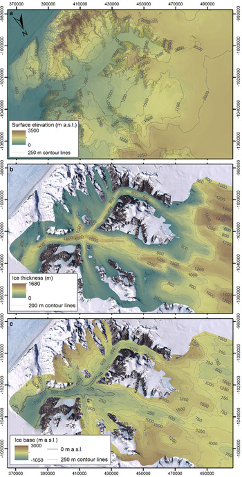
Fig. 6. (a) Surface elevation, (b) firn layer corrected ice thickness and (c) ice base elevation (floating and grounded) within the DHGS. Coordinates are in a Polar Stereographic projection with true scale at 71°S.
The geometric model of the DHGS (Fig. 6) illustrates that the thickness of the Darwin Glacier exceeds 1200 m in several parts of the central valley, while the Hatherton Glacier has ice thicknesses generally between 600 and 900 m in the deepest regions (Fig. 6b). As a consequence, large parts of the Darwin Glacier, the lowermost regions of the Hatherton Glacier and several tributary glaciers are flowing over beds below the current sea level. Further upstream, ice drainage from the EAIS and into the DHGS is restricted by high subglacial ridges resembling a hanging valley wall (Fig. 6c). As the ice flows over these subglacial ridges and into the two main valleys of the DHGS, it thins to <200 m, except at the upper Darwin Glacier, where the model suggests the presence of a prominent ~10 km wide and 1000 m deep subglacial canyon. Unfortunately, the longitudinal ice thickness profile does not follow the central flowline in this region, and it is possible that the geometry model overestimates the depth of the subglacial canyon away from cross profiles.
4.4. Ice velocity
A general downstream increase in ice velocity occurs along the center flowline of the Darwin Glacier, with velocities of <30 m a−1 in the wide upper regions and up to 55 m a−1 at profile C (Fig. 5). Unfortunately, velocity measurements near the outlet of the glacial system were largely unreliable due to a short 2 d measurement period. The dataset provided by Rignot and others (Reference Rignot, Mouginot and Scheuchl2011b) does however show that velocities reach a maximum of ~110 m a−1 at The Nozzle, and center flowline velocities decrease from ~80 m a−1 at profile D to ~45 m a−1 at the predominantly floating profile E. The decrease in ice velocity downstream of the grounding line probably relates to the decrease in surface slope observed at this location (Fig. 4). The ice flow of the Hatherton Glacier is much slower than the Darwin Glacier with a measured velocity of <10 m a−1 along the center flowline at profile G (Figs 2, 5). On the Hatherton Glacier, Rignot and others (Reference Rignot, Mouginot and Scheuchl2011b) have center flowline velocities increasing from ~2 m a−1 at profile F to ~12 m a−1 at profile H.
4.5. Ice flux
Flowlines and medial moraines are clearly visible where blue ice is exposed at the glacier surface (Fig. 1) and provide an indication of the relative contribution of various ice sources. Flowlines on the Hatherton and Darwin Glaciers suggest that mountain glaciers located in the Britannia Range as well as the Touchdown and McCleary Glaciers (Fig. 1) constitute important sources of ice. This is evident on the Hatherton Glacier where a slight increase in ice flux appears to occur downstream despite a negative SMB (Fig. 5). Flowlines at the confluence of the Darwin and Hatherton Glaciers indicate that the Hatherton Glacier contributes little to the overall ice discharge of the glacial system, which instead appears to be dominated by ice draining through the Darwin Glacier valley from the EAIS. This is confirmed by the low calculated ice flux of 0.02 ± 0.01 km3 a−1 at the Hatherton Glacier confluence with the Darwin Glacier (profile H, Fig. 5).
The calculations of ice flux along the Darwin Glacier show that it increases from 0.22 ± 0.04 to 0.27 ± 0.05 km3 a−1 between profiles A and C as various tributaries join the main glacier (Figs 1, 5). A decrease in ice flux appears to occur between profiles C and D despite an additional inflow of ice from a southern tributary glacier. The decrease may be a result of negative SMB in this region, or it could relate to the uncertainties associated with the ice flux calculations. No cross profile exists at the central Darwin Glacier grounding line, and the ice flux increases slightly between upstream cross profile D and downstream cross profile E. The Darwin Glacier receives little additional ice between profile D and the central grounding line, whereas a large inflow of ice occurs from the Gawn Ice Piedmont between the central grounding line and profile E (Fig. 1), explaining the larger ice flux for the lowermost cross profile. As the effect of SMB and basal melting between profile D and the grounding line is negligible compared with the uncertainty associated with the ice flux calculations, the Darwin Glacier ice discharge can be approximated by the 0.24 ± 0.05 km3 a−1 found for cross profile D.
4.6. Surface mass balance
Mass-balance states of Antarctic glaciers are often assessed from a comparison of the catchment-wide SMB and calculated ice discharge (Fricker and others, Reference Fricker, Warner and Allison2000; Rignot, Reference Rignot2002; Wen and others, Reference Wen and Jacka2008). The cumulative catchment-wide SMB of the DHGS has been calculated from four models with varying attributes and spatial resolutions (Table 1). van de Berg and others (Reference van de Berg, van den Broeke, Reijmer and van Meijgaard2006) used output from a regional atmospheric climate model, while Arthern and others (Reference Arthern, Winebrenner and Vaughan2006) relied on an interpolation between in situ measurements guided by a background field derived from satellite data. The two highest resolution models presented by Lenaerts and others (Reference Lenaerts, Van Den Broeke, Scarchilli and Agosta2012a, Reference Lenaerts, van den Broeke, van de Berg, van Meijgaard and Kuipers Munnekeb) are based on regional atmospheric climate models and include the effect of snowdrift, which is highly dependent on the input topography and hence model resolution (Lenaerts and others, Reference Lenaerts, Van Den Broeke, Scarchilli and Agosta2012a).
Table 1. Model resolution, modeled period and DHGS catchment-wide SMB for four different SMB models
The three lowest resolution models all predict positive SMB throughout the DHGS with balance fluxes of between three and six times the Darwin Glacier ice discharge of 0.24 ± 0.05 km3 a−1 calculated by the present study. The observed difference cannot be explained by basal melting of grounded ice within the glacier catchment, which is unlikely to exceed 0.02 km3 a−1 (Riger-Kusk, Reference Riger-Kusk2011). In comparison, the highest resolution model published by Lenaerts and others (Reference Lenaerts, Van Den Broeke, Scarchilli and Agosta2012a) suggests a 2009 catchment-wide SMB which compares reasonably well with the calculated ice discharge. This model includes some ablation within the glacial catchment, although these regions do not coincide with visible blue ice areas.
4.7. Ice shelf basal melting
Downstream of the Darwin Glacier grounding line, the floating ice comes into contact with relatively warm ocean water and basal melting increases. The average basal melt rate for floating ice between the central grounding line and profile E can be estimated from the difference in ice flux through common ice corridors in cross profiles D and E (estimated from flowlines in Fig. 1) and by accounting for surface ablation and mass loss from basal melting under grounded ice. When disregarding the inflow of ice from Gawn Ice Piedmont (~0.03 km3 a−1 ice through profile E), an ice loss of 0.026 km3 a−1 occurs between common ice corridors in profiles D and E. New calculations of ablation rates within blue ice areas in the region (Riger-Kusk, Reference Riger-Kusk2011) suggest that no more than 0.001 km3 a−1 ice is ablated between profiles D and E. The rate of basal melting under grounded ice downstream of profile D is estimated to range between 0.009 m a−1 (minimum basin-wide average) and 0.4 m a−1 (near grounding line) as found by Joughin and others (Reference Joughin2009) for the thicker and faster moving Pine Island and Thwaites Glaciers. Subtracting the ice loss due to surface ablation and basal melting in grounded regions from the total mass loss results in an average basal melt rate of 0.3 ± 0.1 m a−1 for the first 8.5 km downstream of the Darwin Glacier grounding line. As the ice thickness decreases most rapidly close to the grounding line, the basal melt rate at this location probably exceeds the average value. The basal melt rate calculated here for the Ross Ice Shelf downstream of the Darwin Glacier grounding line is considerably smaller than the 1 m a−1 found near the fjord entrance to the David Glacier (Frezzotti and others, Reference Frezzotti, Tabacco and Zirizzotti2000; Wuite and Jezek, Reference Wuite and Jezek2009) and the >10 m a−1 documented near deeper grounding lines of faster moving TAM outlet glaciers (Rignot and Jacobs, Reference Rignot and Jacobs2002; Kenneally and Hughes, Reference Kenneally and Hughes2004). The low melt rate may be explained by limited inflow of warm ocean water due to the comparatively shallow Darwin Glacier grounding line depth, the valley and seafloor topography or influences on ocean temperature and salinity caused by the nearby rapidly melting Byrd Glacier.
5. DISCUSSION
5.1. Characteristics of the Darwin Glacier grounding zone
Due to a lack of radar measurements across Antarctic grounding zones, studies of glacier mass balance often have to rely on ice discharges determined from an assumption of hydrostatic equilibrium where variations in surface slope indicate a change to floating conditions (Rignot, Reference Rignot2002; Rignot and others, Reference Rignot2008; Stearns, Reference Stearns2011; Shepherd and others, Reference Shepherd2012). The new ice thickness measurements collected at the outlet of the DHGS allows for an assessment of the potential error associated with this approach. Previous studies of the Antarctic grounding line have placed the Darwin Glacier central grounding line 1.2 km (Bindschadler and others, Reference Bindschadler2011) and 1.5 km (Scambos and others, Reference Scambos, Haran, Fahnestock, Painter and Bohlander2007) downstream of the position measured in this study, and consequently within the ~2.5 km zone where the ice is elevated above hydrostatic equilibrium. Ice thicknesses calculated from an assumption of hydrostatic equilibrium at the central grounding line locations of Bindschadler and others (Reference Bindschadler2011) and Scambos and others (Reference Scambos, Haran, Fahnestock, Painter and Bohlander2007) exceed ice thickness measured at these locations by 195 and 170 m, respectively. Furthermore, calculated ice thicknesses at the two locations differ from the measured central grounding line ice thickness by +33 and −26 m, respectively. At the central Darwin Glacier grounding line location determined in this study, calculated ice thickness overestimates measured thickness by 280 m due to the significant elevation of the ice above hydrostatic equilibrium. The latter discrepancy is much larger than the average error of 80 ± 20 m previously reported for Antarctica (Rignot and others, Reference Rignot2008, Reference Rignot, Mouginot and Scheuchl2011a). The potential for error at the Darwin Glacier is well illustrated when comparing the previously approximated ice discharge of 1.03 km3 a−1 (Humbert and others, Reference Humbert, Greve and Hutter2005) with the 0.24 ± 0.05 km3 a−1 determined by the present work from measurements of ice thickness and ice velocity close to the central grounding line. Correct positioning of grounding lines is important not only in ice discharge calculations, but also when modeling the ice flow behavior. When Anderson and others (Reference Anderson, Hindmarsh and Lawson2004) applied their flowline model to the DHGS, they used the then available ADD dataset (ADD-Consortium, 2000), which places the Darwin Glacier grounding line more than 20 km downstream of the position presented in this study. This is likely to have introduced errors in the modeled glacier behavior in this region and consequently in changes in ice velocity and thickness over time, the latter of which is the main focus of the study.
The conditions at the grounding zone are further complicated by the gradual transition from fully grounded to fully floating conditions, illustrated by the partially grounded cross profile collected ~8.5 km downstream of the central grounding line. Similar gradual transitions have been observed elsewhere in the TAM and in Antarctica in general (Hughes and Fastook, Reference Hughes and Fastook1981; Bindschadler and others, Reference Bindschadler2011; Marsh and others, Reference Marsh, Rack, Golledge, Lawson and Floricioiu2014). The presence of grounded ice downstream of the central grounding line has implications for the stability of the Darwin Glacier grounding line and may explain the deviation from hydrostatic equilibrium observed in the region. The stability of the ice is also influenced by the shape of the upstream bedrock topography. Most studies agree that several stable grounding line positions may exist over rough bedrock topography, and that grounding lines are generally unstable on beds sloping downwards inland (Weertman, Reference Weertman1974; Schoof, Reference Schoof2007). The central Darwin Glacier grounding line is currently positioned on a slightly upwards-sloping bed, and like other TAM, outlet glaciers are stabilized to some degree by the buttressing effect offered by the Ross Ice Shelf and the surrounding valley walls (Golledge and others, Reference Golledge, Marsh, Rack, Braaten and Jones2014). As a consequence, the Darwin Glacier grounding line appears stable in its current state. Nevertheless, large parts of the DHGS are currently grounded below sea level, and the undulating nature of the bed suggests that the glacial system has the potential for episodes of rapid grounding line retreat.
Our detailed investigations of ice characteristics at the Darwin Glacier grounding zone show that the region is characterized by an abundance of basal crevasses and a downstream development of near horizontal basal terraces. While the formation of basal crevasses is well understood (Jezek and Bentley, Reference Jezek and Bentley1983; Rist and others, Reference Rist, Sammonds, Oerter and Doake2002; Catania and others, Reference Catania, Hulbe and Conway2010), the origin of the basal terraces is less clear. The terraces have similarities to those found in radar measurements collected by Peters and others (Reference Peters, Blankenship and Morse2005) downstream of the Ice Stream C grounding line and by Dutrieux and others (Reference Dutrieux2014) on the Peterman Glacier ice shelf. In the latter study, basal terraces were also observed by an autonomous underwater vehicle under the Pine Island Glacier ice shelf (Dutrieux and others, Reference Dutrieux2014). The terraces found at the base of both Peterman and Pine Island Glacier ice shelves, were located close to sub-ice-shelf channels, a feature which has been described by Le Brocq and others (Reference Le Brocq2013). There is no evidence of sub-ice-shelf channels in any of the radar profiles collected downstream of the Darwin Glacier grounding line, and the development of basal terraces and sub-ice channel systems appear unrelated. The geometry of the basal terraces differs somewhat from that described by Dutrieux and others (Reference Dutrieux2014), who observed larger terrace walls (20–75 m) and smaller widths (20–300 m). The formation mechanisms of the basal terraces remain unknown, although Dutrieux and others (Reference Dutrieux2014) suggested that differences in melting between the horizontal terraces (low melting) and the steep terrace walls (high melting) act to maintain the features, and may even play a part in their creation. This would imply that the observed differences in terrace geometry relate not only to changes in basal topography close to sub-ice-shelf channels, but also to variations in basal melt rates and the age of the feature. The calculated average melt rate of 0.3 ± 0.1 m a−1 for the Ross Ice Shelf downstream of the Darwin Glacier grounding line is significantly less than the ~40 m a−1, documented near the deeper grounding line of Pine Island Glacier (Rignot and Jacobs, Reference Rignot and Jacobs2002) and may contribute to the observed differences. The longitudinal GPR profile (Fig. 3) shows that the widths of the basal terraces increase with distance downstream from the heavily crevassed Darwin Glacier grounding zone. This suggests that a complex interaction between crevasse formation at the grounding line and subsequent differential basal melting and/or freezing is responsible for the creation of basal terraces. The findings presented here provide further support to the hypothesis proposed by Dutrieux and others (Reference Dutrieux2014) that basal terraces might be generic features of ice shelves, which have remained undocumented until recently due to the low resolution of air-borne radar systems.
5.2. Glacier morphology and ice flow behavior
The presented measurements of ice thickness illustrate an undulating bed topography, where the ice thins and thickens as it flows over large bumps and troughs, respectively. Ice thicknesses exceed 1000 m in the central regions and are generally larger than the values applied by Anderson and others (Reference Anderson, Hindmarsh and Lawson2004) from calculations of balance ice fluxes. While there is evidence to suggest that ice drainage into the Darwin Glacier valley is through a prominent subglacial canyon, ice thins to <200 m toward the head of the Hatherton Glacier. The Hatherton Glacier is thinner and has a lower surface slope than the Darwin Glacier, and ice velocities are lower as a result. Evidence presented here shows that the glacier moves with <10 m a−1 in the central regions, corresponding well with the Antarctic-wide map of ice surface velocities which has ice velocities of <15 m a−1 on the Hatherton Glacier (Rignot and others, Reference Rignot, Mouginot and Scheuchl2011c). The new evidence differs from the 40 m a−1 measured previously just upstream of the confluence with the Darwin Glacier (Hughes and Fastook, Reference Hughes and Fastook1981), and as there is no other evidence to suggest a recent change in flow dynamics, is believed to reflect uncertainties in the measurements. The results presented here show that ice thickness, ice velocity and consequently ice flux are low at the entrance to the Hatherton Glacier valley, leaving the glacier particularly sensitive to changes in ice flow from the EAIS. Glacier deposits at the head of the DHGS show that the ice surface of the EAIS close to the TAM may have been up to 100 m above present-day levels during the LGM (Bockheim and others, Reference Bockheim, Wilson, Denton, Andersen and Stuiver1989; Denton and Hughes, Reference Denton and Hughes2000). It is possible that the increased ice flux into the Hatherton Valley could have caused the Hatherton Glacier to advance into adjacent ice-free valleys.
While the Hatherton valley cross-section shape changes little along the length of the glacier, a prominent change occurs along the Darwin Glacier, which has a wide and irregular bed in the uppermost regions, a downstream development of a deep inset trough that changes into a simple U-shaped valley toward the glacier outlet. Measured velocities are highest in the deepest regions and correspond well with both the Antarctic-wide map of ice surface velocities (Rignot and others, Reference Rignot, Mouginot and Scheuchl2011c) and the measurements conducted by Hughes and Fastook (Reference Hughes and Fastook1981). The presence of a central inset trough in the upper regions of the glacier likely reflects the positive feedback of increased glacial erosion in the thickest and fastest parts (Kessler and others, Reference Kessler, Anderson and Briner2008). This effect would be accentuated by central warm-based conditions as was modeled by Anderson and others (Reference Anderson, Hindmarsh and Lawson2004) for the Darwin Glacier, and has been found elsewhere for TAM outlet glaciers with ice thicknesses above 1000 m (Golledge and others, Reference Golledge, Marsh, Rack, Braaten and Jones2014). Further downstream, the U-shaped valley is characteristic of regions that have experienced prolonged glacial erosion. The change in valley shape is indicative of a downstream increase in glacial erosion as the ice thickness and ice velocity increases, and a similar downstream change has been documented for the slow-moving Taylor Glacier located further north in the TAM (Kavanaugh and others, Reference Kavanaugh, Cuffey, Morse, Conway and Rignot2009). From the glacial deposits surrounding the DHGS, it is clear that the ice thickness has varied significantly over the last ~1–2 Ma, probably resulting in large temporal changes in the dynamic behavior and consequently the erosional strength of the glacial system. The current valley shape may reflect past erosional conditions, and further investigations are required in order to establish the present-day basal temperature regime.
5.3. Mass balance of the DHGS
The mass balance of the DHGS was investigated by comparing the new ice discharge with catchment-wide SMB from four SMB models at spatial resolutions ranging from 55 to 5.5 km (Arthern and others, Reference Arthern, Winebrenner and Vaughan2006; van de Berg and others, Reference van de Berg, van den Broeke, Reijmer and van Meijgaard2006; Lenaerts and others, Reference Lenaerts, Van Den Broeke, Scarchilli and Agosta2012a, Reference Lenaerts, van den Broeke, van de Berg, van Meijgaard and Kuipers Munnekeb). The three lowest resolution models suggest an unrealistically large positive mass balance for the DHGS, illustrating the significant uncertainties associated with applying low-resolution models in complex regions. Although inconsistencies exist between ablation areas as suggested by the highest resolution mass-balance model (Lenaerts and others, Reference Lenaerts, Van Den Broeke, Scarchilli and Agosta2012a) and blue ice areas on the DHGS, this model produces a cumulative catchment-wide SMB, which is only slightly higher than the ice discharge calculated by this study. This could suggest a small positive mass balance for the DHGS, although the difference between the two values is within the uncertainties of the calculations. Previous studies of mass balances of TAM outlet glaciers have documented no major positive or negative imbalances (Frezzotti and others, Reference Frezzotti, Tabacco and Zirizzotti2000; Rignot, Reference Rignot2002; Rignot and others, Reference Rignot2008; Wuite and others, Reference Wuite, Jezek, Wu, Farness and Carande2009; Todd and others, Reference Todd, Stone, Conway, Hall and Bromley2010; Stearns, Reference Stearns2011), and the results presented here are likely to reflect inaccuracies in SMB models and calculated discharge. Uncertainties in mass-balance models have been shown to increase in areas with particularly low or high SMB and for small catchment basins (Shepherd and others, Reference Shepherd2012). It is clear that high-resolution models in combination with field measurements of accumulation and ablation rates are essential in order to determine SMB in regions such as the TAM where large spatial variations in topography and SMB occur.
6. CONCLUSION
By combining high-resolution GPR data with measurements from a relatively low-resolution airborne radar survey, we have recorded detailed information about the internal and basal structures of the DHGS and clear readings of ice thicknesses of close to 1700 m. In conjunction with the ice velocity measurements, this has allowed for a detailed description of changes in ice characteristic across the Darwin Glacier grounding zone and a construction of new maps of ice thickness and bed topography for the DHGS. The results have also helped to establish controls on ice flow behavior and facilitated an assessment of the current mass balance of the glacial system.
Results show that both the Hatherton and Darwin Glaciers are somewhat restricted in inflow from the EAIS by subglacial mountains, over which ice thins to <200 m except in the central regions of the Darwin Glacier. The Hatherton Glacier is thinner, flatter and slower moving than the Darwin Glacier and flows in a simple U-shaped valley. By contrast, the Darwin Glacier valley narrows and deepens toward the outlet as velocities reach a maximum of 110–120 m a−1 (Hughes and Fastook, Reference Hughes and Fastook1981; Rignot and others, Reference Rignot, Mouginot and Scheuchl2011c). The position of the central Darwin Glacier grounding line was determined from changes in ice base characteristics, and confirmed by calculations of hydrostatic equilibrium. Upstream of the grounding line, the DHGS is grounded on bedrock which is below sea level for more than 40 km inland. Downstream of the grounding line, the crevasses that characterize the ice base close to the grounding zone are replaced by near horizontal basal terraces. The calculated ice discharge of 0.24 ± 0.05 km3 a−1 compares well with the catchment-wide SMB from a high-resolution mass-balance model (Lenaerts and others, Reference Lenaerts, van den Broeke, van de Berg, van Meijgaard and Kuipers Munneke2012b), and there is nothing to suggest a major mass imbalance at the DHGS.
The glaciological study of the DHGS presented here provides important new information about the varying ice flow within the glacial system, and hence contributes toward a better glaciological understanding of flow behavior of outlet glaciers in the TAM.
ACKNOWLEDGEMENTS
All data presented in this paper are available upon request to author Mette K. Gillespie (mette.kusk.gillespie@hvl.no). We would like to thank Antarctica New Zealand for providing financial and logistical support during the fieldwork and Education New Zealand who funded the PhD study of Mette K. Gillespie through their New Zealand International Doctoral Research Scholarship. W. Rack was partially supported by the Past Antarctic Climate and Future Implications program. IPY ICECAP data collection was funded by National Science Foundation grant PRL-0733025 and National Environmental Research Council grant NE/D003733/1 (PI: Martin Siegert). We also want to thank Martin Siegert who helped coordinate and plan the airborne radar survey (UTIG contribution number 3132). Thank you also to Dean Arthur and the staff at Scott Base for offering the support required to carry out the ground-based fieldwork. The SPIRIT DEM was made available through the IPY (International Polar Year) ASAID (Antarctic Surface Accumulation and Ice Discharge) project (PI: Robert Bindschadler), while Jan Lenaerts made his SMB models available for our calculations of catchment-wide SMB. Parts of this work rely on open access to data made public by authors via the Antarctic Digital Database, the National Snow and Ice Data Center and PANGEA: Data Publisher for Earth & Environmental Science.


 Open access