


Introduction
Levees (Figs 1 and 2) and en-echelon-type shear planes (Figs 1 and 3) are common features in snow avalanche deposits. Levees form as avalanche snow, usually at the avalanche front, is pushed to the side, constructing self-made sidewalls parallel to the main flow direction. The sidewalls consist of snow granules and typically form on slopes flatter than 25°. The levees confine the flow and prevent the avalanche mass from laterally spreading. However, the flow within the sidewalls continues to move forward, penetrating further in the run-out zone (Fig. 4). The interior surface of the sidewalls is rubbed smooth by the flow; frictional heating generates water, which eventually refreezes, creating hard, sculptured ice surfaces. The shear planes are striated and often gouged by debris (rocks, wood) that has been entrained in the flow. The scratch marks are parallel to the basal surface, suggesting that at the shear plane the upper regions of the flow are laminar and plug-like (Fig. 2). The flow channel eventually drains as the mass supply from the tail stops, leaving the sidewalls fully or partially exposed (Fig. 1). The resulting depositional form can have a long, fingerlike appearance, often referred to as 'flow fingers' or 'flow arms' (Fig. 4).

Fig. 1. Levee and en-echelon shear plane formation of a large wet snow avalanche deposited in the Incron channel of the Swiss Vall´ee de la Sionne test site, 30 December 2009. The en-echelon shear planes probably developed first near the avalanche front as it entered the deposition zone. Mass from the tail continued to flow slowly on top of the existing deposits, creating the levee sidewalls shown in the picture. The levee channels drained completely (inset), leaving the sidewalls fully exposed. The mean slope angle is ∼20°. (Photograph: F. Dufour, SLF.)

Fig. 2. Snow avalanche levees, as seen from the inner channel. Note the granular nature of the deposits and the wall striations. (a) Levees formed during the deposition of a spontaneous avalanche that occurred at the Swiss Vall´ee de la Sionne test site in December 2010. The picture looks up towards the Crˆeta Besse 1 and 2 release zones. (b) Levees and granular deposits of the Urezza avalanche, Puschlav, February 2009. (Photograph: Bartelt, SLF.)

Fig. 3. (a) An array of en-echelon shear planes in a small dry snow avalanche, Fl ¨uelatal, near Davos, Switzerland. Note how the shear lines extend outward from the flow centre. (b) A close-up view of the en-echelon faults with ski pole for scale. The picture shows size as well as strike and dip angles. (Photograph: Glover, SLF.)

Fig. 4. (a) Levees formed in theGiglistock Milan avalanche of 12 May 2012. The levees are located in the transition zone above the run-out zone and the skier. (b) Flow fingers with rigid sidewalls developed as the levees drained, exposing the interior side of the shear plane. The drainage fingers ran far on a flat slope. Note the granular characteristics of the deposits. (Photograph: C. H¨anggeli; provided to the authors by T. Stucki, SLF.)
En-echelon-type shear planes also form during the deposition process, as the frontal lobes stall and spread laterally in the run-outzone. Similarto levees, well-defined shear planes develop at the flow boundaries; however, unlike levees, en-echelon shear planes are not parallel to the main flow direction. Typically, several planes form at once, forming a distinctive array of wrench faults (Fig. 3). Levees can be considered concordant structures, since their orientation is parallel to the flow direction; en-echelon planes are discordant structures, in the sense that they are oriented sideways with respect to the flow.
Levees and en-echelon shear planes form when there is an imbalance in the mass flux across the cross section of the avalanche. The combination of a drop in mass flux and the increased frictional work rate at the outer border creates a shearing of the avalanche mass laterally. Thus, part of the avalanche has stopped (the outer mass comprising the levees) while the interior part of the mass continues to flow (the mass within the levee-bound channel; Fig. 5). The boundary between the two masses is the levee line separating the flowing from the non-flowing snow. En-echelon shear planes are governed by a similar formation process, while their orientation moves towards the strike of the basal shear plane, away from the zone of the main flow (Fig. 6). Again, similarly to levees, a discrete height gradient exists across the shear plane. Typically, the lower plane is wrenched away from the upper plane, indicating the mass at the lower plane continues to move.

Fig. 5. Schematic drawing showing the avalanche in the x-y coordinate system of the model. The inset depicts the saddle point in the RU phase space. The line a–b separates the flowing and stopping solution trajectories predicted by the model. In region L, solution trajectories stop (levee formation), whereas in region C of the phase space (channel) the avalanche continues to move. The mass comprising the stationary material we denote with a minus sign; the mass within the levee bound channel we denote with a plus sign. The width of the flowing snow mass is 2b(x).
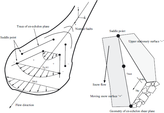
Fig. 6. Schematic drawing showing the avalanche in the x-y coordinate system and the formation of en-echelon shear line. The inset depicts the dip and strike angle of the plane. Because we use a depth-averaged model we consider only the trace of the en-echelon line in the x-y plane. The mass comprising the stationary material we denote with a minus sign; the still-moving mass we denote with a plus sign. The width of the avalanche is 2b(x).
Another observation is that flow levees often form on slopes of moderate, often constant, slope angle. For steep slopes all the flow mass will continue to flow in the downhill direction, while for flatter slopes all the mass will stop. A model for levee/en-echelon formation must therefore allow for two entirely different flow states for a single slope angle and material constants. Both flow states are necessary to develop the mass flux gradients across the avalanche flow width where shear planes can form. A slope angle where mass continues to flow but likewise can stop implies that the rheological behaviour of flowing snow cannot be described by a frictional model with constant flow parameters, independent of the momentary mass flux (avalanche velocity and flow height). For example, to take such material behaviour into account, Reference Mangeney, Bouchut, Thomas, Vilotte and BristeauMangeney and others (2007) modelled the onset of levee formation using the empirical friction law proposed by Reference Pouliquen and ForterrePouliquen and Forterre (2002).
Some recent attempts to explain the process of levee formation (Reference Pouliquen, Delour and SavagePouliquen and others, 1997; Reference Gray and KokelaarGray and Kokelaar, 2010; Reference Johnson, Kokelaar, Iverson, Logan, LaHusen and GrayJohnson and others, 2012) have suggested that particle size segregation is the reason for the mass flux gradients and the formation of the shear planes: larger particles segregate to the upper regions of the flow, where they are transported to the avalanche front and then pushed aside, stop and form levees. While this is a plausible explanation it has several difficulties for snow avalanches. Firstly, particle size measurements in snow avalanches reveal that levees (stopped flow) have the same particle size distribution as the channelized portion of the moving flow (Reference Bartelt and McArdellBartelt and McArdell, 2009). This is visible in Figure 3, where the en-echelon shear planes have formed with no observable gradient in particle sizes. Thus, levees in snow avalanches appear to form independent of the particle size segregation. Even avalanches with relatively homogeneous particle sizes can form these distinct avalanche deposition features. Although we do not question the role of particle size segregation in levee formation, it fails to describe the basic frictional mechanism causing the initiation of the stopping phase. Plastic flow might also be a candidate for the description of levee formation, especially for wet snow avalanches (Reference KelfounKelfoun, 2011). However, as noted by Reference Johnson, Kokelaar, Iverson, Logan, LaHusen and GrayJohnson and others (2012), plastic yielding neglects the influence of the internal flow dynamics or spatial heterogeneities in the flow structure. The deposits of wet snow avalanches are composed of granules (Reference Bartelt and McArdellBartelt and McArdell, 2009) that exhibit no evidence of internal shearing or yielding. Observations indicate that shearing begins predominately at granular interfaces; moreover, the material does not yield.
To understand when and how levee and en-echelon shear planes are formed in avalanches requires a flow model that naturally exhibits this 'stick-slip' behaviour: at some slope angle and flow velocity, the levee sidewalls 'stick' on the slope, whereas the snow in the interior continues to flow, or, is 'slipping' down the slope. Mathematically, this suggests a bifurcation phenomenon within a nonlinear dynamical system - the avalanche (Reference Leine and NijmeijerLeine and Nijmeijer, 2004). The levee sidewalls and flow in the interior channel represent two entirely different equilibrium states of the avalanche. The sidewalls are motionless and in static equilibrium, whereas the channel flow is (nearly) in dynamic equilibrium. The formation of the sidewalls represents the trivial solution to the avalanche dynamics equations, whereas the mathematical solution for the channel interior is a non-trivial stationary solution. A saddle point mathematically separates the two equilibriums, so the shear plane becomes a geometric representation of the bifurcation. Solution trajectories of the mathematical model must bifurcate at the shear plane to one (the trivial) or the other (the non-trivial) solution to form a levee.
Flow bifurcations (Reference Issler and GauerIssler and Gauer, 2008; Reference Bartelt, Meier and BuserBartelt and others, 2011) have been identified in the snow avalanche dynamics model of Reference Christen, Kowalski and BarteltChristen and others (2010) and Reference Bartelt, Bühler, Buser, Christen and MeierBartelt and others (2012). This model explicitly accounts for the role of velocity fluctuations associated with the random movements of the snow granules. We note that levees and en-echelon shear planes are found predominately in granular avalanches (Figs 1 and 2). In fact, levee sidewalls consist of compressed granules that are smoothed by the sliding mass (Fig. 2). Thus, the granular properties of the avalanche appear to play a significant role in levee formation (Reference Pouliquen, Delour and SavagePouliquen and others, 1997; Reference Félix and ThomasFelix and Thomas, 2004; Reference Gray and KokelaarGray and Kokelaar, 2010). In this paper we model flow friction as a process involving the decay of granular kinetic energy during the deposition process (Reference Buser and BarteltBuser and Bartelt, 2009). This physical process leads to strong mass flux gradients across the flow and therefore to large frictional stresses at the flow boundaries, that can initiate flow bifurcations and the subsequent formation of the levees. To find the location of the shear planes in avalanche deposits, therefore, requires knowledge of the avalanche flow velocity, U, and the kinetic energy associated with random particle movements, R. Parameters U and R are linked, because R controls frictional processes and therefore the velocity and stopping behaviour of the flow (Reference Bartelt, Bühler, Buser, Christen and MeierBartelt and others, 2012). We exploit the nonlinear feedback between U and R to show that a saddle-point equilibrium point exists, that separates the flowing and stopping phases of flow in the run-out zone. We compare the results of the mathematical model with laser- scan measurements of avalanche deposits to calculate the measured flow velocities of the avalanches.
Shear Plane Formation
To mathematically treat the formation of levees and enechelon shear planes we must introduce some simplifications to the problem:
-
We treat the avalanche as a planar problem (Fig. 5), projecting all height (z-direction)-dependent variables on to the running surface (the x-y plane) using a depthaveraging procedure. For the friction we use the value of shear stress at the running surface, disregarding the z-dependence. The flow density is constant.
-
The flow width of the avalanche is divided into small flow segments, which flow with a mean depth-averaged velocity, U(x, y, t). The width of the avalanche in the y-direction (perpendicular to the flow direction, x) is 2b(x, t). For the y-dependent velocity, it is possible to use any distribution for U(x, y, t) with zero velocity at the boundary; however, we shall assume, for illustration, a Hagen–Poiseuille (parabolic) profile
where Ū(x, t) is the mean velocity at position x:
-
Therefore, the velocity profile varies along the path of the avalanche in the x-direction (Figs 5 and 6). The avalanche moves fastest at the centre line (y = 0) and is slower at the edges (y = ±b). The flow centre line is arameterized by the slope angle, φ(x). The selection of a parabolic profile, U(x, y, t), is equivalent to assuming a homogeneous, viscous fluid between the edges of the flow and the sidewalls. The local form of the velocity profile depends on surface roughness and terrain undulations, so deviations from an ideal viscous fluid will certainly be observed.
-
Because we use a depth-averaging procedure, the height, H(x), of the flowing snow is given. Be aware that there is no y-dependence of flow height, H. In this case the mass flux in the y-direction depends only on the velocity profile. The height of the levees is the frozen (velocity zero) height of the flow. The levees are exposed as the flow material drains between the sidewalls. The levee sidewalls represent the flow height, H, at that position when the levees form.
-
We assume a flat-bottom flow surface with no terrain undulations. The friction parameters of the model account for surface roughness.
We now turn our attention to the small y-segments across the flow width of the avalanche defined above, making them infinitely small, such that we can consider them mass points. When the avalanche moves, the mass points trace lines in the x-y plane. The mass per unit area, M, is given by the product of the density, ρ, and flow height, H(x): M = ρH(x).We treat the snow flow along the line using the model formulation developed by Reference Bartelt, Buser and PlatzerBartelt and others (2006, Reference Bartelt, Bühler, Buser, Christen and Meier2012), Reference Buser and BarteltBuser and Bartelt (2009) and Reference Christen, Kowalski and BarteltChristen and others (2010):
where gx is the gravitational acceleration in the downslope direction, gx =g sin φ. The model parameters, α and β, control the production and decay of random kinetic energy, R, respectively. The production parameter, α, partitions the shear work rate per unit area, SU, into thermal energy and random energy. The decay coefficient, β, describes how the energy, R, is destroyed by particle interactions. The shear stress, S, is given by a simple Coulomb friction relationship:
where μ is the dry Coulomb friction coefficient accounting for influence of fluctuation energy, R, i.e. gz=g cos φ. The friction coefficient, μ 0, is the static Coulomb friction coefficient, μ(R = 0) = μ 0, associated with the mean density, ρ, with zero fluctuation energy. Parameter R 0 takes into account that the fluctuation energy, R, has greater effect when the weight of the avalanche (flow height) is smaller; R 0 scales the energy, R, by the avalanche weight, R 0 = ρgzH. To model levees, Reference Mangeney, Bouchut, Thomas, Vilotte and BristeauMangeney and others (2007) employed an empirical friction law without consideration of the physical processes governing the decay of random energy in the deposition zone.
In order to predict the formation of the levee and enechelon lines it is not necessary to solve the coupled equations (Eqns (3) and (4)) for U(t) and R(t) using the constitutive equation for shearing, S (Eqn (5)). To find the mass flux gradients across the width in the flow x-direction it is only necessary to investigate the stability of the coupled equations. We seek the time stability of eventual (U, R) solutions (Reference Boyce and DiPrimaBoyce and DiPrima, 1977). There exists a saddle point (U∊ , R∊ ) where for values (U, R) above the levee line, a–b, the avalanche will continue to flow (Fig. 5, ‘+’ region). Conversely, for values (U, R) below the levee line, a–b, the avalanche segment will eventually stop (Fig. 5, ‘−’ region). We will assume that the avalanche segment in the x-direction will stop at once when (U, R) is in the stopping region, because all solutions eventually decay to the trivial solution, U = 0 and R = 0. Moreover, at the saddle point we assume one side suddenly stops (U(x, y) = 0), although it will still have some velocity that must go to zero. This means that in the model the interior will slip at the sidewalls (as observed). The slip velocity is equal to the saddle-point velocity. In this case the shear plane and the bifurcation point are identical. Thus, we will find a line, y∊ (x), where the avalanche has stopped on one side and on the other side the avalanche still flows. The levee forms with flow height H(x) and has the form of a rectangular block (Fig. 7). Details such as changing levee geometry during the stopping are not considered, as we assume the mass stops instantaneously.

Fig. 7. The process of levee formation. At time t = t0 the avalanche is flowing at position x with velocity U(x, y, t 0) and flow height H(x, t 0). The half-width of the avalanche is b(x). A shear plane forms at time t = t 0 at position y = y∊ because R ≤ R∊ and U ≤ U∊ . The interior of the channel drains, exposing the levee sidewalls. The height of the levee is therefore H(x, t 0). Because the production of R depends on the shear work, the maximum R is located at the centre line.
The saddle point, (U∊ , R∊ ), is found by setting Eqns (3) and (4) to zero (dU/dt = dR/dt = 0). We find
and
To find the stability of this equilibrium point we construct the Jacobian matrix of Eqns (3) and (4) at the point (U∊ , R∊ ) and find the eigenvalues of this matrix (Reference Boyce and DiPrimaBoyce and DiPrima, 1977). The eigenvalues are real and of opposite sign, indicating the saddle point we are seeking (see Reference Bartelt, Meier and BuserBartelt and others, 2011, for details). Solution curves approach (U∊ , R∊ ) and then diverge. At low velocity, U, and low R value, solutions converge to the stopped avalanche case (U∊ , R∊ ) = (0, 0) (Fig. 5).
To find the location of the shear line in the avalanche, y∊ , we equate the mass flux at y, Q(x, y, t), with the critical mass flux at the saddle point, MU∊
by which we can find the distance
The levee line, y∊
, is a fraction of the half flow width, b. The quantity ![]() is the mean mass flux at x:
is the mean mass flux at x:
When ![]() is large then y∊ ≈ b; moreover, the levee line exists at the very boundary of the flow. Such behaviour has been observed in videos of avalanche fronts (Fig. 8). The constant, c, is given by
is large then y∊ ≈ b; moreover, the levee line exists at the very boundary of the flow. Such behaviour has been observed in videos of avalanche fronts (Fig. 8). The constant, c, is given by

Fig. 8. (a) The transition zone at the front or interior of the avalanche, where levees or en-echelon lines form. (b) Snapshot from a video showing an avalanche front with levee transition zone. The dashed curves delimit the moving and stopped avalanche mass. (c) Closeup of the frontal lobe of the Salezer avalanche from aerial imagery (B¨uhler and others, 2009). The mass at the outer edges of the flow has stopped, but the interior channel continues tomove, descending a steep slope. Note the orientation of the levee lines in this region. They are not parallel but move inward, indicating a non-constant mass flux across the transition zone.
The displacement speed, ![]() , of the saddle point is
, of the saddle point is
Be aware that the velocity, ![]() , is the velocity of the saddle point in the x-y plane. Importantly,
, is the velocity of the saddle point in the x-y plane. Importantly, ![]() is the movement of a flow state describing the transition between the flowing and stopping regimes. It is not the velocity of the mass, which is zero in the y-direction. By following the saddle point we are able to trace the shear planes in the avalanche deposits. When
is the movement of a flow state describing the transition between the flowing and stopping regimes. It is not the velocity of the mass, which is zero in the y-direction. By following the saddle point we are able to trace the shear planes in the avalanche deposits. When ![]() , W = 0 and the en-echelon shear planes are in line with the mean mass flux,
, W = 0 and the en-echelon shear planes are in line with the mean mass flux, ![]() . We define flow levees to have the special property ∊(x) = 0 (concordant), where ∊ is the angle with respect to the flow direction that the shear plane makes at position x. They require a steady mass flux,
. We define flow levees to have the special property ∊(x) = 0 (concordant), where ∊ is the angle with respect to the flow direction that the shear plane makes at position x. They require a steady mass flux, ![]() . The fact that levees form for stationary flow states has been observed in the granular experiments of Reference Félix and ThomasF´elix and Thomas (2004). However, as we move the saddle point from the edges of the flow into the interior with velocity W, the avalanche mass does not suddenly stop. The saddle-point analysis provides us only with the certainty that the mass will stop, not with the exact stopping time. When the mass flux is not constant, this stopping time becomes important. In an interval of time, Δt , the saddle point displaces inward WΔt ; in the same interval of time, the avalanche displaces UΔt . To find the location of the shear lines when the mass flux is not constant, we must consider this downward displacement. Thus, the angle ∊ is given by
. The fact that levees form for stationary flow states has been observed in the granular experiments of Reference Félix and ThomasF´elix and Thomas (2004). However, as we move the saddle point from the edges of the flow into the interior with velocity W, the avalanche mass does not suddenly stop. The saddle-point analysis provides us only with the certainty that the mass will stop, not with the exact stopping time. When the mass flux is not constant, this stopping time becomes important. In an interval of time, Δt , the saddle point displaces inward WΔt ; in the same interval of time, the avalanche displaces UΔt . To find the location of the shear lines when the mass flux is not constant, we must consider this downward displacement. Thus, the angle ∊ is given by
En-echelon shear planes have the property that ∊(x) ≠ 0 (discordant) and therefore ![]() . They start at the boundaries and move towards the interior of the flow. Faults can exist, which are perpendicular to the flow direction, ∊(x) = ∞ (normal faults). These occur in strongly decelerating avalanches when the velocity, U, is small and much less than W (Fig. 9).
. They start at the boundaries and move towards the interior of the flow. Faults can exist, which are perpendicular to the flow direction, ∊(x) = ∞ (normal faults). These occur in strongly decelerating avalanches when the velocity, U, is small and much less than W (Fig. 9).
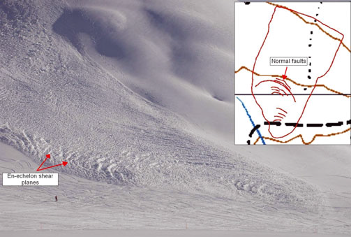
Fig. 9. An array of en-echelon shear planes in the Grünhorn (Davos) avalanche of 12 February 2012. The avalanche was artificially released. We have no velocity information. Many of the shear lines run normal to the flow direction, forming a downward-shaped parabola (inset). The levee model predicts this will occur in stronglydecelerating flows when the mass flow velocity, U, is near zero and smaller than the saddle-point velocity, W. The downward-shaped parabolic form of the shear lines indicates a parabolic-shaped velocity profile, in which the velocity is highest at the flow centre and decreases towards the edges. The shear lines start from the exterior edges of the flow, where the velocity is smallest, and move inwards and upwards where the velocity is highest, forming an array of normal faults. The authors walked the shear lines with a handheld GPS to determine their location and orientation. (Photograph: Feistl and Glover, SLF.)
Examples
Levee formation in VdlS avalanches 816/817
On 6 March 2006 two dry flowing avalanches were artificially released at the Swiss Vall´ee de la Sionne (VdlS) test site. The first avalanche (No. 816) was released at 10:00 from two VdlS release zones (Crˆeta Besse 1 and Pra Roua). The second avalanche (No. 817) was released 50 min later from the third and remaining VdlS release zone (Crêta Besse 2). Both avalanches were large, with fracture heights of ∼1m and release volumes of >100 000m3; both avalanches reached peak front velocities of >50ms−1. Ground surfaces in the transition zone were visible, suggesting considerable snow-cover entrainment in both events. Pre- and post-event aerial laser scans of the avalanche release and deposition zones were performed (Reference Bartelt, Bühler, Buser, Christen and MeierBartelt and others, 2012), providing information on the mass distribution in the run-out zone and counter-slope (Fig. 10). Levees are clearly visible in the deposition zone, extending over the entire run-out zone leading up to the counter-slope (Fig. 10). A particularly distinctive feature of the deposits is the flow arm that bendstowards the orographic right-hand side of the main VdlS run-out zone. This flow arm with levee sidewalls extended from the front of avalanche 816. Interior levees, behind theavalanche front, are clearly visible at the tail of the deposits, far upslope of the leading edge of the avalanche. The interior levee drained, exposing the levee sidewalls. The drained mass stopped in the middle of the deposits, piling up to >5m in height. This levee arose from the tail of avalanche 817. Note that both the front and interior tail levees exhibitremarkably parallel sidewalls. Post-event granule counting was undertaken to quantify the granulometric dimensions of the avalanches (Reference Bartelt and McArdellBartelt and McArdell, 2009).

Fig. 10. Two- and three-dimensional depictions of aerial laser scans of VdlS avalanches 816/817. Levees formed at the front of avalanche 816 and at the tail of avalanche 817.
To investigate the levee structures in more detail, we constructed lateral profiles across the aerial laser scans at three specific locations in the depositions (profiles P1, P2 and P3; Fig. 10). Profile P1 was selected at the tail of the avalanche deposits and represents a drained, interior levee (Fig. 11a). A prominent, 2m high levee sidewall formed on the orographic right-hand side of the avalanche, approximately in the middle of the flow channel. The sidewall on the opposite side appears to be initiated on the steep channel side, indicating that terrain features that restrict the avalanche mass flux can cause the formation of levee lines. (Our simple model assumes a flat bottom and does not account for terrain undulations that would cause a change in the mass flux.) The distance between levees is 2y∊ = 36m, and we estimate the half-width of the flow (on the flat terrain) to be 2b = 60m. The average slope in the avalanche flow direction across the profile is 25°. With these data we could apply Eqn (9) to predict the mean avalanche flow velocity when the levee formed. Velocity profile measurements (Reference Kern, Bartelt, Sovilla and BuserKern and others, 2009) were used to determine the granular fluctuation energy production (α) and decay (β) parameters of Reference Buser and BarteltBuser and Bartelt (2009). These are α = 0.1 and β = 0.65 s−1. We emphasize that these are not model fit parameters, but parameters deduced from independent measurements. The values have been likewise applied to numerically simulate these and similar avalanche events (e.g. Reference Christen, Kowalski and BarteltChristen and others, 2010; Reference Bartelt, Bühler, Buser, Christen and MeierBartelt and others, 2012). We find mean velocities between Ū = 3.1 and 4.1ms −1 for Coulomb friction values between μ 0 = 0.577 and 0.620. Model results are reported in Table 1. We emphasize that this velocity range is in good agreement with measured tail velocities (see Reference Kern, Bartelt, Sovilla and BuserKern and others, 2009).

Fig. 11. Levee profiles of VdlS avalanches 816/817 obtained from aerial laser scanning. Profiles are defined in Figure 10. (a) Profile P1. Drained levee. (b) Profile P2. Partially drained levee. (c) Profile P3. Independent flow arm with levee arising from front of avalanche 816.
Table 1. Summary of levee examples from VdlS avalanches 816 and 3003/3004

Profile P2 (Figs 10 and 11b) was selected because it is partially filled by channel flow mass and not fully drained. The 3–4m levee sidewalls are clearly visible in the laser scans; they are located 2y∊ = 32m apart. The distance between the levee sidewalls did not change substantially as the avalanche moved between profiles P1 and P2 (from 36 to 32 m). The estimated flow width of the avalanche is slightly larger (to 2b = 77 from 60 m), but this is to be expected, as the mean slope angle has flattened somewhat (from 24.9° to 19.3°), causing a slight spreading of the frontal lobe. We applied the same calculation procedure (Eqn (9)) with the same model parameters as above, to determine the avalanche flow velocity using the measured levee dimensions. We find that a mean velocity of Ū = 7.4ms−1 is required to form levee sidewalls of this dimension at this slope angle (Table 1). If the flow plug within the channel cannot reach this velocity, then the flow plug must eventually stop, as the mass flux is inadequate to construct the levees. Or, levees with a smaller spacing between sidewalls are created within the existing levee (see Fig. 11, where there appear to be several levees within levees). The measured deposition substantiates this result as the channel flow piles up immediately after profile P2.
Profile P3 (Figs 10 and 11c) represents a levee structure that was created at the avalanche front as it defines the maximum reach of the avalanche. The avalanche arm has a flow width of 2b = 23m and the levee sidewalls are spaced 2y∊ = 10m apart. The mean slope angle of this profile is 19.2°. From the laser-scan data, we estimate the flow heights of the flow arm to be H ≈ 2.5m. Again, using the above model calculations, we find the calculated mean velocity to be between Ū= 7.7 and 8.9ms −1. These velocities are possible as the measured peak front velocities reached by the avalanche before it began to decelerate were ∼50ms −1 (Reference Kern, Bartelt, Sovilla and BuserKern and others, 2009). Numerical simulations of avalanche 816 with the same model parameters reveal velocities of ∼15ms −1 in this region of the deposits (Reference Bartelt, Bühler, Buser, Christen and MeierBartelt and others, 2012). The levee model calculations reveal that higher mass fluxes are required to form levees at flatter lope angles. Such higher mass fluxes can only be found at or near the avalanche front, providing an explanation of why levees and flow arms often extend beyond the bulk of the avalanche deposits, defining the maximum reach of the avalanche.
Levee formation in VdlS avalanches 3002, 3003 and 3004
Over a 24 hour period bridging 6 and 7 December 2010, three avalanches released spontaneously at the VdlS test site No. 3002 (6:22, 6 December 2010), No. 3003 (18:31, 6 December 2010) and No. 3004 (3:36, 7 December 2010). Because of bad visibility in the VdlS release zone it was not possible to identify the avalanche release zones and reconstruct the events in detail, but an aerial laser scan of the deposition zone was possible (Fig. 12). Measurements at the mast revealed flow velocities at the tail of 5ms −1. Manual observations of the deposition zone were also performed by the authors on 10 December 2010. At the time of release, air temperatures were below zero and the size, shape and hardness of the granules in the levee channels led us to conclude that the deposits arose from dry, flowing avalanches (Reference Bartelt and McArdellBartelt and McArdell, 2009). In the deposition region, the avalanches were running on the ground and the flow was sensitive to terrain undulations and variations in surface roughness, which affected the lateral mass flux, producing several flow fingers.

Fig. 12. Two- and three-dimensional depictions of aerial laser scans of VdlS avalanches 3003/3004.
The laser-scan measurements (and manual observations) reveal a braided-type deposition pattern with two prominent levee structures. The first levee structure is located at the very tail of the deposits. It starts above the measurement pylon, where significant mass pile-up is visible. A well-defined frontal lobe is located somewhat downslope, suggesting that this levee arose from the tail, but stopped at the pylon. The second levee structure penetrated deep into the runout zone, almost reaching the valley bottom. At the end of this levee, the channel mass piled up and made a 90° turn, running on a dirt road with smoother surface before stopping. It is possible that the two levee structures were generated by two different avalanches. In our analysis, we only considered the second levee.
We made three lateral profiles of this levee, placing profile P1 near the formation region, profile P2 in the middle and profile P3 behind the mass pile-up. The distance between the levee sidewalls remained remarkably constant, 2y∊ ≈ 20 m; the flow width increased slightly as the slope angle decreased (Fig. 13).We again applied Eqn (9) to predict the critical flow velocity at the time of levee formation, taking the dry snow avalanche parameters of the first example (α = 0.1, β = 0.65, μ 0 = 0.577; Table 1), to find a critical velocity of U = 5.4ms −1. This mean velocity is slightly larger than the observed tail velocity of 5ms−1. Higher saddle-point velocities are found at profiles P2 and P3, indicating the levee formed in the region of profile P1 and created smaller levee widths as the avalanche moved down slope to profiles P2 and P3.

Fig. 13. Levee profiles of VdlS avalanche 3004 obtained from aerial laser scanning. Profiles are defined in Figure 12. (a) Profile 1. Drained channel. (b) Profile 2. Partially filled channel. (c) Profile 3. Behind the channel pile-up. The laser-scan profiles indicate levees within levees.
Salezer wet snow avalanche, 23 April 2008
On 23 April 2008 a large wet snow avalanche ran down the Salezer torrent of Dorfberg, Davos. Several fracture slabs released spontaneously from multiple release areas, creating a large event. The avalanche mass ran out of the confined torrent into an open run-out area, splitting into two separate flow arms, (Fig. 14). The orographic left arm was smaller and, before stopping, was deflected by a small avalanche dam constructed to protect the houses of the Meierhof settlement. The orographic right arm formed levee sidewalls spaced 2y∊ = 45m apart; the total flow width was 2b ≈ 60 m, but widened as the avalanche ran out on flatter terrain (Fig. 15) . The orographic right sidewall was prominent, ∼3.5m high and 10m wide. The orographic left sidewall was lower and often difficult to identify in the laser scans. The deposit contained a series of striations running parallel to the flow direction, suggesting that the avalanche constructed a series of levees as itmoved forward. This indicates an uneven mass flux across the flow width of the channel flow. The levee channel contains three regions, similar to the regions of the interior levee of VdlS avalanches 816/817: a drained channel at the tail of the flow, a channel mass pile-up at the tip of the frontal lobe and a transition region between the drained zone and the wet snow mass pile-up.

Fig. 14. Optical imagery and aerial laser scans of Salezer (Davos) avalanche of 23 April 2008. A 45m wide levee structure formed as the avalanche departed the torrent channel. Definition of levee profiles P1, P2 and P3.

Fig. 15. Levee profiles of Salezer avalanche (Davos) of 23 April 2008. Deposition profiles were obtained from aerial laser scanning with 0.5m resolution; however, only a 2m digital terrain model is available. Profiles are defined in Figure 14. (a) Profile P1. Drained levee. (b) Profile P2. Partially drained levee. (c) Profile P3. Avalanche lobe.
A significant feature of the Salezer avalanche deposits is the tongue-like structure at the very front of the avalanche. The 70m wide avalanche stopped on a flat slope, just above a steeper track section. Because the mass in the interior channel was moving faster, it was able to descend the steep slope, moving ∼20m before coming to a standstill; mass on the outer edges of the avalanche stopped on the flat slope and remained stationary above the tongue. This deposition feature provides evidence for a mass flux distribution that decreases towards the outer edges of the avalanche. A closer inspection of aerial photographs of the tongue (Fig. 8) reveals levee lines that are not parallel but move inward, toward the channel centre.
We again applied the saddle-point model to determine the avalanche velocity as it exited the Salezer torrent, the location where the levee initiated. We used wet snow avalanche parameters, α = 0.1 and β = 1.00 (i.e. higher dissipation of fluctuation energy because of the larger plastic deformations of the wet snow granules; when random energy decays, it dissipates to heat) and μ 0 = 0.400 (i.e. lower Coulomb friction because of the lubricating effect of thepore-water). Similar values have been used to back-calculate wet snow avalanche events in VdlS (Reference Christen, Kowalski and BarteltChristen and others, 2010). The model predicts that a velocity of U = 9.9ms−1 is required at, or behind, the avalanche leading edge. The avalanche front could have been travelling at a higher velocity, the levees forming behind the head. This is a plausible result. We also predicted the velocities required to maintain the levee structure on the downslope profiles P2 (transition) and P3 (pile-up) (Table 1). At profile P2 a velocity of 15.9ms −1 is required; at P3 a velocity of 24.8ms −1. It is unlikely that these velocities were reached anywhere within the avalanche at this stage, and therefore the channel mass was strongly decelerating, leading to the observed mass pileup at the frontal lobe.
En-echelon shear plane formation
The mining of snow accumulations by explosives in the Fl ¨uelatal forms part of the regular programme of avalanche mitigation in Davos. Heavy snowfall in combination with a strongly wind-blown period on 4 March 2011 required the artificial release of several avalanches in this area. Together with the piste control service of Davos, a series of dry snow avalanches in open mountain fan terrain were observed and documented. In all, four avalanches were released, each demonstrating the formation of en-echelon shear planes, with orientations both parallel and oblique to the principal flowline. Using a Trimble GeoXH 6000 mobile DGPS (differential GPS) and laser range finder, the trace of the en-echelon shear planes, inundated area and crown of the avalanches were mapped (Fig. 16). Additionally, the structure of the shear plane surfaces was inspected, capturing strike and dip data and the throw along the slip planes, along with striated surfaces (Fig. 3).

Fig. 16. Overview of the Flüelatal avalanche of 4 March 2011, showing location of the en-echelon shear lines with respect to the avalanche inundation area. At the location of the en-echelon shear planes the avalanche was flowing with a width of 50m and velocity of ∼10ms −1.
When the en-echelon shear planes formed, the avalanche was flowing at a width of 2b = 50m with constant flow heights of H ≈ 1m. The traces of the en-echelon shear planes commence ∼6.2m inward of the outer edge of deposits and extend up to 18.5m long. They cease before the internal edge of the deposits, approaching the core of the avalanche where the basal shear plane is stripped free of snow by the flow. The trace of the shear planes intersects the flow path at 41° (Fig. 16).
Shear planes dipped, on average, 56° and ranged between43° and 73°. Striation lineations on the shear plane surfaces intersect the strike of the shear planes by 40°, and, with up to 0.5m between the foot and the hanging wall, the surfaces were wrenched in an oblique slip motion around 0.9malong the slip plane (Fig. 3). In all, there were eight en-echelon shear planes in this avalanche zone.
Using the measured data (b = 25m, y∊ = b − 6.2 = 18.8m) we predicted the maximum speed of the avalanche as the en-echelon shear lines formed at the outer edge of the flow. We took constitutive parameters α, β and R0
for dry avalanches (Reference Buser and BarteltBuser and Bartelt, 2009; Reference Christen, Kowalski and BarteltChristen and others, 2010), α = 0.1 and β = 0.6s
−1. The energy parameter, R0, scales with the normal stress, ρgzH, R
0 = 2.7 kPa. For the friction constant, μ0, we took values used by Reference Bartelt, Meier and BuserBartelt and others (2011) to simulate avalanches, taking μ0 = 0.577 (friction angle 30°), which corresponds to Coulomb friction values measured by Reference Van Herwijnen and HeierliVan Herwijnen and Heierli (2009) or Reference Platzer, Bartelt and KernPlatzer and others (2007). Using Eqn (9) and these values, it was possible to calculate the mean mass flux, ![]() , and therefore the mean velocity, at the time of the shear line formation, U = 10.5ms
−1. This value is confirmed from back-analysis of video footage of the avalanche, where velocities in the upper portion of the slope were up to 11ms−1. From the equations, we predict that the propagation (starting at the edges and running towards the centre of the flow) of the shear planes was ∼9ms
−1, taking ∼1 s for them to form. The avalanche front, which could cover 10m in this second, stopped after the shear lines formed. It was not possible to observe the formation of the planes in the captured video, due to the presence of the avalanche powder cloud. To confirm this, further detailed observations of the formation of the en-echelon shear planes should be made.
, and therefore the mean velocity, at the time of the shear line formation, U = 10.5ms
−1. This value is confirmed from back-analysis of video footage of the avalanche, where velocities in the upper portion of the slope were up to 11ms−1. From the equations, we predict that the propagation (starting at the edges and running towards the centre of the flow) of the shear planes was ∼9ms
−1, taking ∼1 s for them to form. The avalanche front, which could cover 10m in this second, stopped after the shear lines formed. It was not possible to observe the formation of the planes in the captured video, due to the presence of the avalanche powder cloud. To confirm this, further detailed observations of the formation of the en-echelon shear planes should be made.
Conclusions
The above developments represent a systematic and quantitative description of levee and en-echelon shear plane formationin snow avalanches. It is of considerable importance that the same theory as is used to model avalanche velocity andrun-out (Reference Christen, Kowalski and BarteltChristen and others, 2010), flow regime transitions (Reference Issler and GauerIssler and Gauer, 2008; Reference Bartelt, Meier and BuserBartelt and others, 2011) and flow dilantancy (Reference Buser and BarteltBuser and Bartelt, 2011) can also be applied to predict the formation of levee lines, without changing the values of the model parameters governing the production and decay of fluctuation energy in flowing snow. The frictional effects of random kinetic energy appear to be very striking, affording an explanation of many well-known phenomena in snow avalanches and permitting a complete theory of snow flow in natural terrain.
Although the present model is oversimplified for levee formation, it nonetheless models the main features. Firstly, levee formation is sensitive to slope angle. For the same material parameters, higher velocities (mass flux) are required to form levees on flatter slopes. Thus, levees observed in the run-out zone will form at or near the head of the avalanche, where the flow velocities (mass flux) are largest. This occurred in both the VdlS avalanches 816/817 and 3003/3004. On steeper slopes smaller mass fluxes are necessary to form levees. Lower velocities are found at the avalanche tail. This result implies that levees can form at different locations and running times as a function of the evolution of avalanche mass flux between the head and tail. Most likely the formation of levees does not occur solely at the front or tail of the avalanche, but continuously at all stages of deposition, depending on the interplay between the mass flux in the flow direction and the slope angle. This explains the tremendously varied and complex structure of avalanche deposits.
Secondly, in the model we assume a flat bottom with a constant flow height and a Hagen_Poiseuille velocity distribution. As the examples have shown, these assumptions are often far from reality. At ravine sidewalls or gully shoulders, variations in surface roughness will change the mass flux distribution in the flow direction. Natural walls or small ridges in the flow direction are ideal locations for the initiation of levees, because they limit the mass flux and therefore prescribe the location of the saddle point. Thus, the model predicts why levee lines often form on gully sides, the edges of forests or on the sloped surfaces of deflecting dams. The inclusion of such features in avalanche dynamics calculations requires high-resolution digital terrain models (Reference Bühler, Christen, Kowalski and BarteltBühler and others, 2011).
The en-echelon shear lines are also a function of the mass flux evolution. In the example we studied, the first planes formed behind the front. More planes appeared as the avalanche continued to flow downward. The necessary condition for such behaviour is that the mass flux decreases quickly behind the front, probably faster than the change in slope angle, indicating a small avalanche that is starving as mass is continuously lost from the head. The decreasing mass flux gives rise to shear lines that are not parallel to the main flow direction. We note that many flow fingers are similar to en-echelon planes as they are often extruded at some angle to the main flow direction (Figs 10 and 12).
Finally, it is unlikely that avalanche dynamic programs will ever have sufficient numerical resolution to model the formation of levee lines completely, unlike the run-out and flow regime problems, where the resolution of numerical and digital terrain models already appears to be adequate for hazard mapping and other practical applications. Levee lines are discrete, sharp lines that cannot be resolved on calculation grids of several metres. The simulation of levee lines will require high-resolution terrain models to capture natural walls and other small-scale terrain features. It is our hope that the simplified model presented here might help quantify under what conditions levees can form, and therefore provide avalanche experts with additional information on how to read and interpret the very complex features found in typical snow avalanche deposits. As the formation of levees depends on the mass flux, and therefore the frictional properties of the avalanche, it should be possible to retrieve model parameters from levee measurements.


