


Introduction
The Greenland ice sheet, the greatest fresh-water reservoir in the Northern hemisphere, is losing mass at an accelerating rate as a response to climate warming in the Arctic (Vaughan and others, Reference Vaughan2013). This mass loss is responsible for a 0.46–0.76 mm per year rise of global mean sea level in the last decades, or 15–30% of the observed contemporary sea-level rise (Box and others, Reference Box2018; WCRP Global Sea Level Budget Group, Reference WCRP Global Sea Level Budget Group2018; Nerem and others, Reference Nerem2018). Roughly half of the current ice-sheet mass loss stems from surface melt and subsequent meltwater runoff, both of which increased during recent decades (van den Broeke and others, Reference van den Broeke2016). More intense surface melting was accompanied by an increasing melt areal extent (e.g. Mote, Reference Mote2007; Nghiem and others, Reference Nghiem S2012). Greenland's firn is also affected by this expansion of melt area: its ice content increases (de la Peña and others, Reference de la Peña2015; Machguth and others, Reference Machguth2016; Graeter and others, Reference Graeter2018), its density increases (Vandecrux and others, Reference Vandecrux2018), its pore space decreases (van Angelen and others, Reference van Angelen, Lenaerts, van den Broeke, Fettweis and van Meijgaard2013; Vandecrux and others, Reference Vandecrux2019) and its temperature increases (Polashenski and others, Reference Polashenski2014). The combination of these changes lowers the firn's meltwater-retention capacity and its buffering of potential sea-level rise (Pfeffer and others, Reference Pfeffer, Meier and Illangasekare1991; Harper and others, Reference Harper, Humphrey, Pfeffer, Brown and Fettweis2012; MacFerrin and others, Reference MacFerrin2019).
Snow and firn models are often used in combination with Regional Climate Models (RCM) to simulate the snow and firn conditions across the Greenland ice sheet (e.g., van Angelen and others, Reference van Angelen, Lenaerts, van den Broeke, Fettweis and van Meijgaard2013; Langen and others, Reference Langen, Fausto, Vandecrux, Mottram and Box2017; Steger and others, Reference Steger2017; Ligtenberg and others, Reference Ligtenberg, Munneke, Noël and van den Broeke2018; Niwano and others, Reference Niwano2018). However, the validation of these RCM-driven snow models remains challenging due to limited observations. No comprehensive observational dataset of firn temperature has so far been made available. Given the uncertainty in RCM simulations, it is necessary to test snow and firn models with in situ observations to evaluate the overall model performance. At present, our understanding of firn processes is best evaluated by comparing firn models forced by automatic weather station observations to in situ firn observations (Humphrey and others, Reference Humphrey, Harper and Pfeffer2012; Charalampidis and others, Reference Charalampidis2015, Reference Charalampidis2016; Cox and others, Reference Cox, Humphrey and Harper2015; Miller and others, Reference Miller2017; Vandecrux and others, Reference Vandecrux2018).
The evolution of the physical characteristics of the Greenland ice sheet firn has been reasonably well documented; for instance its air content by van Angelen and others (Reference van Angelen, Lenaerts, van den Broeke, Fettweis and van Meijgaard2013), Ligtenberg and others (Reference Ligtenberg, Munneke, Noël and van den Broeke2018) and Vandecrux and others (Reference Vandecrux2019), its stratigraphy by Parry and others (Reference Parry2007), Mikkelsen and others (Reference Mikkelsen2013), Machguth and others (Reference Machguth2016) and MacFerrin and others (Reference MacFerrin2019) and its density by Vandecrux and others (Reference Vandecrux2018). However, the evolution of its temperature has so far only been investigated either at single sites (Pfeffer and Humphrey, Reference Pfeffer and Humphrey1996; Charalampidis and others, Reference Charalampidis2015, Reference Charalampidis2016; Miller and others, Reference Miller2017) and/or over at most two seasons (Humphrey and others, Reference Humphrey, Harper and Pfeffer2012). These studies provided a detailed description of the dominant firn processes at these sites, but could not place their observations into an interannual, geographical or climatological perspective. Polashenski and others (Reference Polashenski2014) compared distributed firn temperature measurements from 2013 and from the 1950's in Northwest Greenland. Their measurements reflected the warm summer of 2012 and revealed a firn warming in the percolation area. However, little is known about the melt and precipitation history between the two periods. The evolution of firn density and temperature profiles on glaciers of the Canadian Arctic (Bezeau and others, Reference Bezeau, Sharp, Burgess and Gascon2013) was found to reduce meltwater retention and enhance mass loss from these glaciers (Noël and others, Reference Noël2018a).
The meltwater retention capacity of the firn depends on three physical characteristics: (i) the availability of pore space to host the meltwater, (ii) the availability of cold content to refreeze the meltwater and (iii) the possibility for meltwater to percolate in deeper firn where conditions (i) and (ii) are met. The firn's cold content is the energy required to bring it to melting temperature. Since meltwater can only refreeze when cold content is available, it represents a key parameter of the firn's meltwater retention capacity. Yet, the magnitude and evolution of the firn cold content of the Greenland ice sheet has not been investigated.
Few locations in the Greenland ice sheet firn area allow the evaluation of firn characteristics. The Greenland Climate Network (GC-Net) automatic weather stations have been operating since the mid-1990s, recording several climate parameters and firn temperatures (Steffen and others, Reference Steffen, Box and Abdalati1996, Steffen and Box, Reference Steffen and Box2001). A few studies have used these observations to document the surface energy and mass balance: Box and Steffen (Reference Steffen and Box2001) at 13 firn sites for 1995–2000, Cullen and others (Reference Cullen, Mölg, Conway and Steffen2014) at one site for 2000–2002 and Vandecrux and others (Reference Vandecrux2018) at four sites for 1998–2015. An important detail is that none of these studies corrected the shortwave radiation measurements for station tilt (Wang and others, Reference Wang, Zender, van As, Smeets and van den Broeke2016). Additionally, the GC-Net firn temperature observations have so far not been used to their full potential, e.g. only as proxy for annual near-surface air temperature (Steffen and Box, Reference Steffen and Box2001; McGrath and others, Reference McGrath, Colgan, Bayou, Muto and Steffen2013).
The depth to which meltwater percolates and therefore the portion of firn cold content that is mobilised for meltwater refreezing varies from millimetres to tens of meters depending on the melt intensity and firn characteristics (Pfeffer and others, Reference Pfeffer, Meier and Illangasekare1991; Humphrey and others, Reference Humphrey, Harper and Pfeffer2012; Charalampidis and others, Reference Charalampidis2016). Additionally, heat conduction allows deep-firn cold content to be indirectly utilised for the refreezing of percolating meltwater closer to the surface. High up in the ice-sheet accumulation area, where most of the GC-Net weather stations are located, liquid-water percolation is found to reach only a few meters depth (1–3 m, e.g., Heilig and others, Reference Heilig, Eisen, Macferrin, Tedesco and Fettweis2018). Hence, only the near-surface firn cold content is utilised. The present study therefore uses the top 20 m firn, which includes all meltwater-percolation events observed at the GC-Net sites, as a definition for the near-surface firn.
In this study, we use gap-filled hourly data from nine GC-Net sites (Fig. 1) located at elevations between 2022 and 3254 m above sea level (a.s.l.) and spanning 15 degrees of latitude on the Greenland ice sheet accumulation area to calculate the surface energy and mass balance over the period 1998–2017. These surface energy and mass fluxes are used to force a firn model that we validate with firn density and temperature observations. We use these firn simulations to describe 20-year-long time series of the top 20 m firn cold content at nine sites across the vast accumulation area of the Greenland ice sheet.
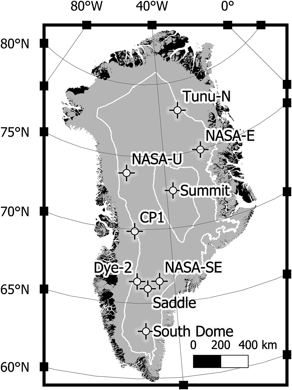
Fig. 1. GC-Net automatic weather stations included in this study. The white lines illustrate the 2000 and 3000 m a.s.l. elevation contours.
Methods
Weather data processing
GC-Net stations measure air temperature, relative humidity, wind speed, atmospheric pressure and downward/upward shortwave radiation. Each GC-Net station has two measurement levels. We use preferably the upper level, located between 0.5 and ~4 m above the surface, because these instruments are less often covered or buried in snow. Exceptions are time periods when only measurements from the lower level are available. We use the outlier rejection and gap-filling procedure from Vandecrux and others (Reference Vandecrux2018). Data gaps in any variable under 6 h are interpolated using polynomial functions. Larger gaps in air temperature, pressure, wind speed, relative humidity and downward shortwave radiation are filled using data, either from nearby weather stations or from RACMO2.3p2 (Noël and others, Reference Noël2018b), adjusted to the available observations. CP2 and Swiss Camp stations (Steffen and others, Reference Steffen, Box and Abdalati1996) were used for gap-filling at CP1, KAN_U station (Charalampidis and others, Reference Charalampidis2015) was used for Dye-2 and the NOAA and ETH stations (Miller and others, Reference Miller2017) were used at Summit. Statistics about the gap-filling process (part of gap-filled data in the final dataset and comparison between gap-filling data and available data) are presented in Supplementary Table S1. Gaps in upward shortwave radiation are filled using downward shortwave radiation and MODIS daily MOD10A1 albedo after Box and others (Reference Box2017) 500 m gridded data. Shortwave radiation observations are corrected for station tilt using the Retrospective Iterative Geometry-Based method from Wang and others (Reference Wang, Zender, van As, Smeets and van den Broeke2016) within the JAWS weather station data processing tool (https://github.com/jaws/jaws). Due to the absence of downward longwave radiation measurements, we use the output from RACMO2.3p2. Downward longwave radiation from RACMO2.3p2 significantly improvement compared to RACMO2.3p1 with a −7.1 W m−2 bias, a root mean squared error (RMSE) of 21.2 W m−2 and a coefficient of determination (R 2) of 0.83 when compared to observations from 23 PROMICE weather stations, mostly located in the ice-sheet ablation area (Noël and others, Reference Noël2018b). These metrics indicate a potential underestimation of cloud cover at lower elevation. Yet, in the absence of sufficient observation from the accumulation area, we do not adjust the downward longwave radiation values or account for a potential temporal mismatch of simulated cloud cover in RACMO2.3p2.
Snow surface height measured by two sonic rangers is used to derive hourly snow accumulation at the surface, either from snowfall or drift events, after Vandecrux and others (Reference Vandecrux2018). The measured surface-height data are noisy, and we smooth those data using a variance filter over a 10-days moving window. After filtering, any increment in surface height is taken as a new snow layer of 315 kg m−3 density (Fausto and others, Reference Fausto2018). We eventually multiply this sonic-ranger-derived accumulation by a site-specific calibration factor so that the derived cumulated winter accumulation matches with 65 springtime snow-pit-derived accumulation observations (7.2 snow pits per site on average, see Table S2). Surface-height variations due to sublimation and deposition are significantly smaller than height changes due to precipitation and drifting, and as such they cannot be measured with the sonic rangers. Instead, sublimation/deposition is calculated from the weather data as detailed in Section ‘Surface-energy-budget calculation’. We find that these calculated sublimation/deposition values have a net contribution to winter mass balance lower than ±3 cm water equivalent (w.e.) at all sites and all years. This further confirms that sublimation/deposition can be neglected when adjusting the sonic-ranger-derived accumulation to snow pits.
At CP1, suspiciously high albedo exceeding 0.85 was measured by the station over the 2005–2009 period (Vandecrux and others, Reference Vandecrux2018). We discarded the upward shortwave radiation measurements over the period 2005–2009 before applying the gap-filling routine, altering the results for CP1 compared to Vandecrux and others (Reference Vandecrux2018).
Surface-energy-budget calculation
The energy available for melt (M) is calculated as the sum of downward and upward shortwave radiation (SR↓, SR↑), downward and upward longwave radiative flux (LR↓, LR↑), the turbulent sensible heat flux, the turbulent latent heat flux and the conductive energy flux to or from the subsurface (G) following van As (Reference van As2011) and Vandecrux and others (Reference Vandecrux2018):

This equation is solvable since it has one unknown variable: surface temperature (T s). LR↑ is calculated from T s using the Stefan–Boltzmann law with a constant surface emissivity of 0.98 (Miller and others, Reference Miller2017, Vandecrux and others, Reference Vandecrux2018). G is calculated from T s and from subsurface characteristics calculated by the firn model (Section ‘Firn model’). The calculation of the turbulent heat fluxes also requires T s and uses the bulk approach accounting for the stability of near-surface atmospheric stratification (van As and others, Reference van As, van den Broeke, Reijmer and van de Wal2005; Vandecrux and others, Reference Vandecrux2018). At each hourly time step, Eqn (1) is solved iteratively either with a subfreezing T s in the absence of melt; or with T s being at melting point and allocating excess energy to melt.
Firn model
We use the firn model from Vandecrux and others (Reference Vandecrux2018), which is based on the firn model of Langen and others (Reference Langen, Fausto, Vandecrux, Mottram and Box2017). The model has 200 vertical layers of varying thicknesses and a layer merging-splitting methodology that ensures a high vertical resolution near the surface where gradients in temperature and density are largest. The minimum layer thickness is 4 cm water equivalent (w.e.). The modelled firn column starts with a total thickness of 40 m w.e. (~70 m). When possible, we initialise the entire model column with observed firn density profiles (Table 1). If the available core is too shallow, we append to this profile densities of 830 kg m-3 at depths of 30 and 70 m w.e. and fit a 2nd degree polynomial function of depth. The shallow profile and the polynomial function are used to initialise the model column. For temperature, the upper part of the model column is initialised using the data from the thermocouple string (Section ‘Accumulation, firn density and temperature observations’), which extends to ~10 m depth. For temperatures in the deeper firn, we use a site-specific 2nd degree polynomial function of depth to interpolate between the deepest available thermocouple measurement and the prescribed deep firn temperature (Table 1) at the bottom of the model. For firn density observations from before 1998 (Table 1), an initial simulation was made between the coring date and 1998 to ensure a valid initial density. For all stations except Summit, these initial runs correspond to the period extending from the installation of the GC-Net station to June 1998, when all nine stations were operational. Filtered and gap-filled observed climate is used as forcing and observed firn density and temperature are used to initialise the model. At Summit, the initial run starts in 1990 but no firn temperature measurement is readily available until 1996, the year when the GC-Net weather station was installed. In the absence of better information about the firn temperature in 1990, the observed 1996 firn temperature profile is used to initialise the run. Further details about these initial simulations are available in Fig. S1 of the Supplementary Material.
Table 1. Deep firn temperature used as the boundary condition of the firn model and details about the firn cores used for initialisation of the firn density in the model

For each layer and on hourly time steps, the model calculates the firn temperature according to heat conduction and storage as well as latent-heat release in case of meltwater refreezing. Unlike in Langen and others (Reference Langen, Fausto, Vandecrux, Mottram and Box2017), the heat capacity and thermal conductivity are calculated from firn temperature and density after Yen (Reference Yen1981). The heat equation is solved with a fixed temperature (Table 1) at the bottom of the model domain (Vandecrux and others, Reference Vandecrux2018). The firn density is updated at hourly time steps accounting for firn compaction derived from overburden pressure (Vionnet and others, Reference Vionnet2012) and for the ice resulting from meltwater refreezing. Meltwater generated at the surface is transferred vertically to underlying layers according to Darcy's law after Langen and others (Reference Langen, Fausto, Vandecrux, Mottram and Box2017). If transferred to a subfreezing model layer with sufficient pore space, water is refrozen and transferred to the layer's ice content, until the latent-heat release brings the layer's temperature to 0°C. The vertical firn water flux depends on the firn irreducible water content (Coléou and Lesaffre, Reference Coléou and Lesaffre1998), the firn's saturated (Calonne and others, Reference Calonne2012) and unsaturated (Hirashima and others, Reference Hirashima, Yamaguchi, Sato and Lehning2010) hydraulic conductivities and on a coefficient that accounts for the effect of ice content on the firn hydraulic conductivity (Colbeck, Reference Colbeck1975; used as in Vandecrux and others, Reference Vandecrux2018). The evolution of grain size, needed to calculate hydraulic conductivity, is calculated from firn temperature and water content according to Brun (Reference Brun1989). Given that our study sites are all well inside the accumulation area, we do not allow lateral meltwater runoff. In the very rare cases where some excess water cannot percolate downward or be held by capillary forces, the water is left ponding in its layer until it eventually percolates or refreezes.
Accumulation, firn density and temperature observations
The firn characteristics are greatly dependent on the local net snow accumulation: snowfall plus deposition minus sublimation. To ensure that the firn model is provided with accurate accumulation values, we compare the net snow accumulation calculated from weather station measurements to 14 firn-core derived accumulation records: Nine cores from PARCA (Mosley-Thompson and others, Reference Mosley-Thompson2001; Bales and others, Reference Bales2009), the ACT-11D core at Dye-2 (Forster and others, Reference Forster2014), Core 14 at NASA-U (Lewis and others, Reference Lewis2019), a core from 2012 at South Dome (Ørum, Reference Ørum2015), the Owen core at Summit (Hawley and others, Reference Hawley2014) and a core from 2007 at CP1 (Porter and Mosley-Thompson, Reference Porter and Mosley-Thompson2014). Some of these cores do not overlap with our study period but can nevertheless be used to ensure that the station-derived accumulation has a realistic magnitude and variability.
The capacity of our firn model to simulate the thermal state of the firn also depends on its ability to reproduce the near-surface firn density. For that purpose, we use 42 firn cores (Table 2) to validate the simulated average density in three depth ranges (0–5 m, 5–20 m and >20 m). We calculate for each depth interval the mean bias, RMSE and R 2 between the simulated and observed average densities. We also use these firn cores to validate the vertically resolved simulated density profiles. Unfortunately, no firn cores were available after 1998 at NASA-E and Tunu-N.
Table 2. Firn cores used to validate modelled firn density

GC-Net stations are equipped with type-T thermocouple strings having a 0.1°C accuracy and 1 m spacing from 0.1 to 9.1 m depth (Steffen and Box, Reference Steffen and Box2001). Records are visually inspected to discard erroneous measurements. Thermocouple temperature measurements are known to be affected by high-frequency noise that originates from voltage instability within the data logger (Sampson, Reference Sampson2009; Cathles and others, Reference Cathles, Cathles and Mr2007). These variations are generally centred around the true temperature, but their magnitude can reach up to several degrees. We remove the most prominent peaks using two successive variance filters (Liu and others, Reference Liu, Shah and Jiang2004): the first one with a running window of one week and variance threshold of 0.05 and the other one with a 6-hour window and a variance threshold of 0.1. Residual noise (within ±1°C) remained after this processing step and was preferred over the removal of real temperature variations through too much filtering. Despite the noise, thermocouple measurements can be used to evaluate the general performance of our firn model. After installation, the depth of each sensor changes as a result of surface and subsurface processes: Snowfall and snow deposition increase the sensors' depth, while melt and sublimation remove surface snow thereby decreasing the sensors' depth. Additionally, the firn in which the sensors are installed undergoes densification as a result of metamorphism and overburden pressure which slightly reduces the sensor spacing. These processes are accounted for in our firn model that we also use to estimate sensors' depth at any point in time to allow comparison with model results.
Firn cold content
A useful indicator of the thermal state of the firn is its cold content, which is the amount of energy needed to bring a volume of firn to melting point. At each time step, we calculate from our simulations the cold content of the top 20 m of firn (CC20, in kJ m−2) as:

where ci = 2.108 kJ kg−1 K−1 is the specific heat of ice, ρ 20 is the volume-weighted average density of the layers composing the top 20 m of firn, T 20 is the mass-weighted average temperature of the layers composing the top 20 m firn and T m is the melting point temperature.
The top 20 m cold content is influenced by various processes. Firstly, the energy flux occurring at the surface and at 20 m depth can either add or draw heat to/from the near-surface firn. This energy is redistributed through the top 20 m of firn through internal heat conduction. Secondly, surface melt takes energy available at the surface and releases it as latent heat in the top 20 m firn when the meltwater refreezes. Thirdly, snow accumulation (snowfall or deposition) at the surface adds low-density fresh snow at the top of the firn column and removes cold, deep firn from the considered 0–20 m depth range. Lastly, ablation (melt or sublimation) removes low density surface snow and adds cold, deep firn to the top 20 m of the firn. In the following, the contributions of these four processes, namely heat conduction, latent-heat release, accumulation and ablation, to cold content are described as positive when they increase the near-surface cold content, either by decreasing firn temperature or increasing firn density. Inversely, negative contributions describe processes that decrease the firn cold content.
Results and discussion
Climatology and surface energy budget
While Vandecrux and others (Reference Vandecrux2018) discovered increasing trends in June through August (JJA) average 2 m air temperatures at four out of our nine sites over the 1998–2015 period, these trends are not present when including 2016 and relatively cold 2017 (Table A1). None of the calculated trends in yearly and seasonal averages are statistically significant (P > 0.2, Table A1). This is due to the cold summers in 2013–2015 and even colder summer of 2017. Within the study period, we note that the JJA average temperatures range between −13.9°C (Summit) and −5.4°C (Dye-2), with 2010–2012 values between 0.7 and 1.7°C warmer than the 1998–2017 average at all nine station sites (Table A1). Albedo, however, decreases significantly (P < 0.05) at six sites out of nine (Table 3). This is predominantly due to the extreme warm summer of 2012, when melt was recorded almost over the entire ice sheet. During that summer the albedo decreased between 2.4 and 10% relative to the average albedo except at Summit and Tunu-N where 2012 summer albedo was close to average (Table 3).
Table 3. Albedo trends and average JJA values at the nine weather station sites over the period 1998–2017 and in 2012

Statistically significant trends (P < 0.05) are displayed in bold.
During the 1998–2017 period, JJA average net shortwave radiation was between 51.8 and 66.9 W m−2 at the weather-station sites, making shortwave radiation the largest energy flux to the surface. The decrease in albedo has caused more shortwave radiation to be absorbed by the surface (Table 3). Indeed, JJA average net shortwave radiative fluxes increased at a rate of 2.8 to 8.1 W m−2 decade−1 at our nine sites (trends with P < 0.05 at NASA-E, Summit, Saddle and South Dome). JJA average net longwave radiation ranges between −30 and −40 W m−2 between sites. The JJA average sensible and latent heat flux contributions range between −3.9 W m−2 at Saddle and 7.9 W m−2 at Tunu-N, and −13.1W m−2 at Dye-2 and −3.5 W m−2 at Tunu-N, respectively. Finally, the conductive heat flux was relatively small, with JJA averages ranging between −8.5 at Tunu-N and 1.9 W m−2 at Dye-2. Energy-budget components and calculated melt are displayed in Fig. S2.
Melt occurred at all sites in the study period, but not in all years (Fig. 2). The highest average annual melt (221 mm w.e. a−1) is found at Dye-2. The site with the lowest and least frequent melting is Summit station, where the average annual melt is <1 mm w.e. per year. Remarkably, Summit experienced melting >1 mm w.e. in 2011, due to several short-lived melt episodes, and in July 2012. In 2012, relatively large melt was calculated at all sites (Fig. 2): more than three times the average annual melt for the warmer sites (CP1, Dye-2) and up to 10 times the average melt at the lower-temperature sites located at higher elevation or latitude (Summit, NASA-E, Tunu-N, NASA-U).

Fig. 2. Annual surface melt calculated at each site with (blue) and without (red) tilt correction of shortwave-radiation measurements. Note the different y-axes.
Correcting shortwave radiation measurements for station tilt considerably impacts the calculated melt at certain stations and in specific years (Fig. 2). South Dome and Tunu-N are the stations that required the most tilt correction, producing respectively +172 and +75% more melt with tilt correction. Due to more frequent maintenance and levelling of the instruments, other stations yield on average +10% more melt with tilt correction.
Snow accumulation
We find decreasing net snow accumulation (snowfall plus deposition minus sublimation) at CP1, Dye-2, NASA-SE, Saddle and South Dome over the period 1998–2017 (Fig. 3). These trends range between −20 and −107 mm w.e. per decade. Only the trend at CP1 is statistically significant (P < 0.05), while trends at the other sites are not significantly different from zero (P > 0.1) potentially because of the high year-to-year snowfall variability and the limited number of years available to calculate these trends. Increasing snow accumulation of +43, +24 and +11 mm w.e. decade−1 are observed at NASA-E, Summit and Tunu-N although these trends are not statistically significant (P > 0.1).

Fig. 3. Annual snow accumulation (snowfall plus deposition minus sublimation) derived from weather stations (black) and from available firn and ice cores (grey). Note the different y-axes for the bottom panels.
The snow accumulation values derived from surface height, adjusted to match the end-of-winter accumulation measured in snow pits, are in good agreement with firn-core derived accumulation records (Fig. 3). Our results confirm the decreasing accumulation found by Lewis and others (Reference Lewis2019) in the firn core and radar data from western Greenland. They calculated a −90 mm w.e. decade−1 snow accumulation trend for the period 1996–2016 and found agreement with the MAR and RACMO2.3p2 regional climate models. This decrease in snowfall is nevertheless restricted to central western Greenland as our northernmost stations show no or positive trends in accumulation. Note that, Wong and others (Reference Wong2015) also showed positive trends in precipitation in Northwest Greenland for elevations below ~1680 m a.s.l..
Firn density
The simulated top 20 m firn density remained relatively stable at the coldest sites (NASA-E, Summit and Tunu-N), while it increased by 2.4 to 7.6% between 2003 and 2012 at warmer sites (Figs 4a–c). After reaching a maximum value in the warm year of 2012, the near-surface firn density decreased at NASA-SE, Saddle and South Dome. At Dye-2 and CP1, density remained relatively high until 2017.

Fig. 4. (a–c) Modelled hourly top 20 m average firn density at the nine study sites relative to their June 2003 value. (d) Modelled vs observed firn densities for three depth ranges. The grey area indicates the ± 40 kg m−3 uncertainty associated with any firn density observation.
Compared against 42 firn density profiles, the simulations have a RMSE of 39 kg m−3 when comparing the top (<5 m) average density, 23 kg m−3 for the mid-depth (5–20 m) and 36 kg m−3 for the deeper firn-core sections (Fig. 4d). When compared to the full-core averages, the model has a 28 kg m−3 RMSE and R 2 of 0.91. The simulated density is on average 13 kg m−3 lower than observed. This low-density bias is stronger for shallow firn (mean bias −24 kg m−3) than for the firn in 5–20 m (mean bias −4 kg m−3) and deep firn (mean bias −14 kg m−3). The simulated density profile, when compared to observations (Fig. S3), reproduces the natural variability of firn density among the nine sites and across depth ranges. Nevertheless, the model cannot reproduce the precise vertical position of observed ice layers. The mismatch probably stems from inaccuracies in surface forcing, model formulation and vertical resolution. The comparison of average densities and density profiles (Figs 4, S3) also suggests that the model deviates more from observations at sites with higher melt and meltwater refreezing (namely CP1, Dye-2, NASA-SE) than at Summit, the only cold site where several cores are available. This deviation could originate from inaccurate meltwater percolation in the model but also from a greater spatial heterogeneity of firn density at these warmer sites. Yet, the general agreement between the simulations and multiple cores indicates that the model provides a good estimation of the average firn conditions in the vicinity of the weather stations.
10 m firn temperature
At most sites and for most years, the model produces 10 m firn temperature time series within the observed envelope of variability (Fig. 5). The site-wise comparisons of firn temperature at each thermistor depth (Fig. S4) have R 2 ranging from 0.65 at South Dome to 0.90 at Tunu-N. The model indicates firn warming at Dye-2, Saddle, South Dome, NASA-E, Summit and Tunu-N by 0.09–1.08°C per decade but cooling between −0.12 and −0.36°C per decade at CP1, NASA-SE, NASA-U. A 4°C warming at Dye-2 follows the extreme warm summer of 2012. However, by 2017 simulated firn temperatures had returned within 1°C of the pre-2012 10 m firn temperature. Most of the thermistor strings were discontinued after 2010. There are therefore no direct measurements of the firn temperatures over the warm summers of 2010 and 2012 at our study sites to validate our simulations. The model presents a cold bias at all sites except Summit. Considering that the 10 m firn temperature observations are dependent on the sensors' depth uncertainty and noise, and that the model result is the outcome of the simulated surface energy balance, refreezing and latent-heat release, heat conduction and snow accumulation at the surface, it is difficult to pinpoint one unique source of uncertainty. Yet, the firn model produces realistic firn temperatures through time and among the sites, allowing the use of the simulations to describe the cold content of the firn at the nine study sites.
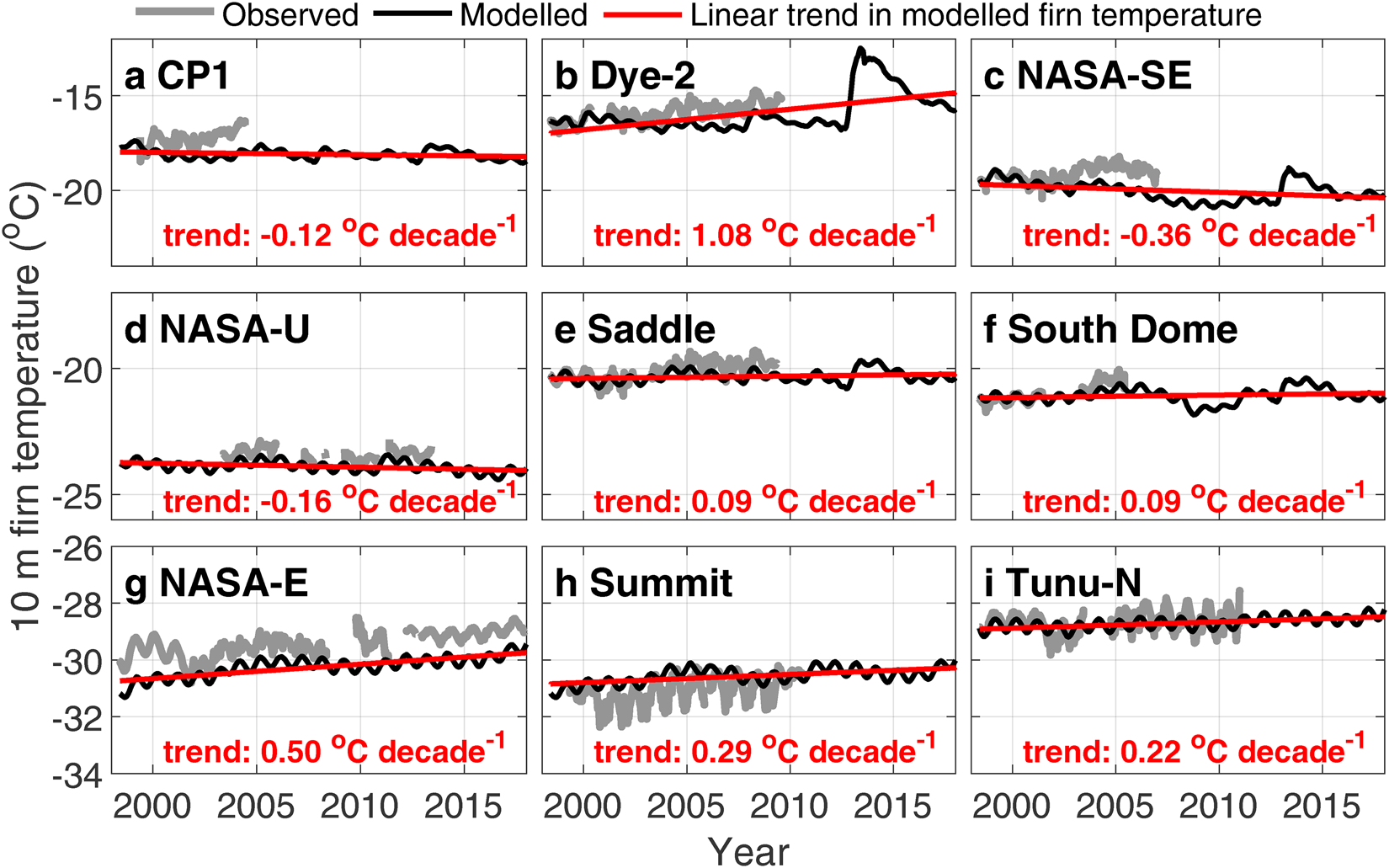
Fig. 5. Observed and simulated 10 m firn temperatures at the nine ice-sheet locations.
Firn cold content
The processes feeding or depleting the cold content vary and sometimes change roles seasonally. We investigate this seasonality by averaging the daily contributions of heat conduction, latent-heat release, snow accumulation and surface ablation (from melt and sublimation) to the top 20 m firn cold content for each day of the year between 1998 and 2017 (Fig. 6). In winter, emission of longwave radiation decreases the surface temperature. The heat is thus conducted predominantly from the subsurface to the surface and contributes to the increase of cold content of the near-surface firn (positive contribution in Fig. 6). In spring, higher air temperatures and increasing shortwave radiation warms up the surface. The heat conduction reverses direction and starts to warm up the firn and to deplete its cold content (negative contribution in Fig. 6). Throughout the year, snowfall deposits low-cold-content fresh snow at the surface, further decreasing the near-surface-firn cold content (negative contribution of accumulation in Fig. 6) as the considered depth range shifts up, excluding deep, cold firn. During summer, the surface snow can be warmed up to 0°C and melt is initiated. Surface ablation through melting and sublimation has a small positive impact on cold content as it removes low-cold-content surface snow in favour of cold firn at 20 m depth (Fig. 6). However, the meltwater is entirely refrozen within the near-surface firn at our sites. Subsequently, the released latent heat has a strong negative impact on the cold content (Fig. 6). Simultaneously, the heat is conducted away from the near-surface firn: downward to deeper and colder firn and upward to the surface where it is emitted back to the atmosphere during nighttime by longwave radiative emission and sensible/latent heat fluxes. At our sites, heat fluxes at 20 m depth are several orders of magnitude smaller than heat fluxes at the surface. Hence, heat conduction typically works to increase the cold content during winter, during the night or during melting conditions when it counteracts the effect of latent-heat release. Nevertheless, the near-surface cold content drastically decreases during melt episodes (Fig. 6).

Fig. 6. 1998–2017 climatology of cold content (grey, right axis) and its main contributors (coloured stacked areas, left axis): heat conduction (red), latent-heat release (yellow), snow accumulation (purple) and ablation (green).
Between 1998 and 2017, firn cold content remained stable (within ±10% of mean values) at all sites except Dye-2 (Fig. 7). At Dye-2, the cold content decreased by 24% after the extreme melt summer of 2012 had warmed the subsurface. Subsequently, it took 5 years for the near-surface firn of Dye-2 to recover its cold content as excess heat punctually released in 2012 was conducted towards the surface or greater depth (Fig. 7). By 2017, the firn cold content at Dye-2 had reached its pre-2012 level. The firn model allows to identify the drivers of these cold content fluctuations. Heat conduction towards the suface or to greater depths adds annually from 9.8 MJ m−2 at Tunu-N to 84.2 MJ m−2 at Dye-2 to the near-surface-firn cold content and is its main positive contributor. On the other hand, snow accumulation, through the addition of warmer, less dense snow at the surface, and the release of latent heat during melt seasons depletes the near-surface firn of cold content. Their relative importance varies from site to site. The latent-heat release is responsible for most of the loss of cold content at relatively low and warm sites such as Dye-2 (−80.8 MJ m−2 a−1) while almost absent at colder sites (~−2 MJ m−2 a−1 at Summit, NASA-E, NASA-U and Tunu-N). The contribution of snow accumulation to cold content ranges from −10 MJ m−2 a−1 at Tunu-N to −25 MJ m−2 a−1 at South Dome and NASA-SE, which not only depends on annual precipitation, but also on the air temperature during precipitation events. Surface ablation (i.e. sublimation and melt) shifts the 20 m depth horizon downward where cold and dense firn is found and is responsible for a low but constant 1–2 MJ m−2 a−1 contribution to the cold content. latent-heat release only plays an important role at Dye-2 (11 MJ m−2 a−1) and a moderate role at CP1, NASA-SE, Saddle and South Dome (4–7 MJ m−2 a−1).

Fig. 7. Cold content (grey, right axis) and cumulative contributions of heat conduction (red), latent-heat release (yellow), snow accumulation (purple) and surface ablation (green). Note the different y-axes for each row.
Cold content is a function of not only temperature, but also firn density (Eqn (2)). Consequently, a 1% increase in firn density will induce a 1% increase in cold content at constant temperature. This co-variation of density and cold content is not accounted for when only the 10 m temperature is used as a proxy for near-surface firn cold content (Polashenski and others, Reference Polashenski2014). This is illustrated at CP1 where, despite a stable 10 m temperature (Fig. 5), the top 20 m firn cold content has actually been increasing by ~10% (Fig. 7). At NASA-U, Summit and Tunu-N, the decline of cold content can be explained by stable firn densities in combination with slight positive trends in 10 m firn temperature. Furthermore, denser firn has a higher thermal conductivity and will redistribute energy faster after a heating event. At Dye-2, about 24% of the top 20 m cold content was depleted during the summer 2012, however it left the firn denser (Fig. 4a), which contributed to the recovery of the lost cold content in subsequent years through more efficient conductive cooling. Although firn densification reduces firn meltwater retention capacity (van Angelen and others, Reference van Angelen, Lenaerts, van den Broeke, Fettweis and van Meijgaard2013; Vandecrux and others, Reference Vandecrux2018), we show that densification can have a positive impact on the cold content and consequently on the firn's meltwater refreezing capacity. Whether cold content or pore space availability will be more important for the overall retention capacity of the Greenland firn is an open question for future research and will depend on local conditions, timing/magnitude of melt and considered timescale.
Considering the intricate relationship between firn density and temperature and their drivers (snowfall, heat conduction, meltwater refreezing), it is misleading to ascribe an increase in firn temperature solely to an increase in melt (e.g. Polashenski and others, Reference Polashenski2014). Although the latent-heat release from meltwater refreezing is the main process decreasing the near-surface cold content for the warmer sites (Fig. 7), the build-up of cold content over the years, the surface energy balance and the accumulation of fresh snow at the surface can also affect firn temperatures and cold content significantly (Fig. 7). Also, should the decrease of precipitation in Western Greenland continue (Fig. 3 and Lewis and others, Reference Lewis2019), one can expect an increase of near-surface cold content in these regions due to denser near-surface firn and enhanced firn cooling in the winter.
We also hypothesise that, in the lower accumulation area of the ice sheet, the recent near-surface firn densification (Fig. 4a) and the stability of the near-surface firn cold content (Fig. 7) promote the emergence of low-permeability ice slabs (Machguth and others, Reference Machguth2016, MacFerrin and others, Reference MacFerrin2019). Indeed, increasing near-surface firn densities, on the one hand, increase the cold content and the thermal conductivity in the near-surface firn, but on the other hand, reduce the volume available for meltwater retention and the firn hydraulic conductivity. All these changes thus promote more intense refreezing into shallow ice features, potentially coalescing into ice slabs if enough melt is provided. Yet the specific climatological and firn conditions required for the saturation of the near-surface firn with ice remain unclear as well as the role of deep, heterogeneous meltwater percolation (Machguth and others, Reference Machguth2016; MacFerrin and others, Reference MacFerrin2019; Verjans and others, Reference Verjans2019).
Conclusion
A gap-free hourly meteorological dataset for the period 1998–2017 was constructed from nine automatic weather stations located in the accumulation zone of the Greenland ice sheet. These time series were used to calculate the surface energy budget and drive a firn model. Calculated net snow accumulation and simulated firn densities compared favourably with firn-core observations. Firn temperature measurements available at the weather stations were corrected for the sensors' depth evolution and highlight a cold bias of the model at all sites except Summit. The output of the firn model showed that the cold content of the top 20 m of firn remained relatively stable (within ±10% of their 1998 values) at all sites except at Dye-2, where a 24% decrease occurred in the summer of 2012. It subsequently took five years for the cold content to recover at Dye-2. Heat conduction toward the surface and/or deeper firn is the main process feeding the cold content during winter, night, and melting conditions at all sites. Yet heat conduction can be directed from the surface to the firn and deplete the near-surface cold content during springtime. By removing low-cold-content surface snow, sublimation and melt had a positive but minor impact on near-surface cold content. The processes depleting the near-surface-firn cold content, however, varied interannually and between sites. Snow accumulation, adding low-cold-content snow at the surface, was the main process depleting the near-surface-firn cold content at relatively low-melt sites, such as NASA-U, NASA-E, Summit, and Tunu-N, or during low-melt years. At sites with more melt, the role of latent-heat release becomes considerable in the yearly loss of cold content budget. It represented up to 86% of all contributions depleting the firn cold content at Dye-2. Heat conduction to deeper firn or back to the surface during nighttime counteracted the summer decrease in cold content. Therefore, the heat balance at the end of the season is a sensitive coupling between surface energy balance, heat conduction through the firn, latent-heat release and snowfall magnitude, and should be cautiously attributed to one or several of these actors. Finally, while it was known that firn densification reduces pore space available for meltwater refreezing, our work illustrates how it also increases the near-surface-firn cold content and potentially sets favourable conditions for near-surface meltwater refreezing. The interaction of weather, firn conditions, and the development of runoff-enhancing features such as ice slabs gives strong motivation to continue climate and firn monitoring in the Greenland ice sheet accumulation area.
Supplementary material
The supplementary material for this article can be found at https://doi.org/10.1017/jog.2020.30.
Data
The GC-Net data are available at http://cires1.colorado.edu/steffen/gcnet. The surface-energy-balance components, gap-filled meteorological variables at standard heights and station-derived snowfall rates are available at https://www.doi.org/10.18739/A2V698C33. The depth-corrected firn temperature observations are available at https://www.doi.org/10.18739/A2GX44V1P. The model output including firn density, temperature, cold content and its contributors can be downloaded at https://www.doi.org/10.18739/A2QF8JJ9B. Most of the firn-core density and accumulation records used in this study are available in the SUMup dataset https://doi.org/10.5194/essd-10-1959-2018 while data from CP_2007, GTC14, SouthDome_2012, Albert_2000, Albert_2007 can be inquired to their respective authors. The source code of the surface-energy-balance and firn model is available at https://github.com/BaptisteVandecrux/SEB_Firn_model.git.
Acknowledgements
This work is part of the Retain project funded by the Danmarks Frie Forskningsfond (grant 4002-00234) and is supported by NASA grants NNX10AR76 G and NNX15AC62G, by DFG grant HE 7501/1-1 and by the Programme for Monitoring of the Greenland Ice Sheet (PROMICE, http://promice.org). We are grateful to G. Lewis and E. Mosley-Thompson for providing some of the firn core data used in this study. We thank F. Covi, an anonymous reviewer and Scientific Editor C. Tijm-Reijmer for their constructive comments on the manuscript.
Appendix
Table A1. Annual and seasonal 2 m air temperature statistics at the nine study sites


 Open access