


Introduction
The flow of glaciers and ice streams is driven by gravity and opposed by resistive forces. Restraining forces acting at the bed result from some unknown combination of “sticky spots” at the ice bed interface, subglacial hydraulic conditions, topographic roughness and rheological properties of the basal material. Sticky spots are localized regions of the bed where the basal shear stress is concentrated and which balance some or all of the applied driving stress (Reference AlleyAlley, 1993).
Data from West Antarctica suggest the presence of sticky spots, which support high basal shear stress, surrounded by a generally well-lubricated, low-shear-strength bed. Force-budget calculations for ice flow at the Byrd Station strain network (Reference Van der Veen and Whillans.Van der Veen and Whillans, 1989), where surface measurements were used to infer stresses at depth, showed that the basal drag is highly variable across the bed and concentrated at a few distinct points. These high-drag, slow-sliding sites are not always correlated with basal topographic highs, indicating that some process such as basal water drainage is involved in governing resistance at the bed. Reference MacAyealMacAyeal (1992) and Reference MacAyeal, Bindschadler. and Scambos.MacAyeal and others (1995) used control methods to invert the observed surface velocity pattern of Ice Stream E for the distribution of subglacial friction. Irregularity of this inferred distribution suggests that ice is not underlain by a uniform layer of deformable sediment and that increased basal friction is introduced by rigid bedrock or by variations in subglacial water pressure. Reference Alley, Anandakrishnan., Bentley. and Lord.Alley and others (1994) suggested that basal water has been diverted away from Ice Stream C, resulting in a disruption of the lubricating water film. They hypothesized that the ice stream has slowed and stopped due to the enhanced basal stress on a few sticky spots at the bed. Neighboring Ice Stream B flows rapidly (400–800 m a1) despite its similarity to Ice Stream C in physical dimensions, accumulation, temperature (Reference Shabtaie, Whillans. and Bentley.Shabtaie and others, 1987) and substrate properties (Reference Rooney, Blankenship., Alley. and Bentley.Rooney and others, 1987; Reference Atre and Bentley.Atre and Bentley, 1993). Reference Anandakrishnan and Alley.Anandakrishnan and Alley (1994) suggest that sticky spots exist beneath Ice Stream B but rarely manifest themselves in the force balance at the bed because they are better lubricated than those beneath Ice Stream C. This conclusion is supported by observations that microseismic events are 20 times more abundant at the base of Ice Stream C than at the base of Ice Stream B (Reference Anandakrishnan. and Bentley.Anandakrishnan and Bentley, 1993). The more frequent occurrence of microseismic events beneath Ice Stream C points to a difference in frictional character of sticky spots between the fast- and slow-moving ice streams.
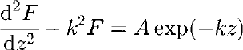
The foregoing discussion highlights the reasons for current interest in the characteristics of subglacial sticky spots and the larger issue of ice–bed coupling. Simultaneous measurements of subglacial water pressure and plough-meter response offer a unique approach to studying the mechanical and hydrological coupling between a glacier and its bed. A ploughmeter is essentially a 1.5 m long steel rod which is driven ~0.1–0.2m into subglacial sediment. The rod will bend elastically if the immersed tip is dragged through the sediment as the glacier slides forward (Fig. 1a). Strain gauges bonded onto the rod register bending in two mutually orthogonal directions (Fig. 1b). Detailed information on the construction, calibration, installation and theory of this device is given in Reference Fischer and Clarke.Fischer and Clarke (1994). Of relevance to the present study is the knowledge that, using the calibration, the bending moment as measured with the ploughmeter can be decomposed into a force applied to the tip and the azimuth of this force with respect to internal coordinates of the device.
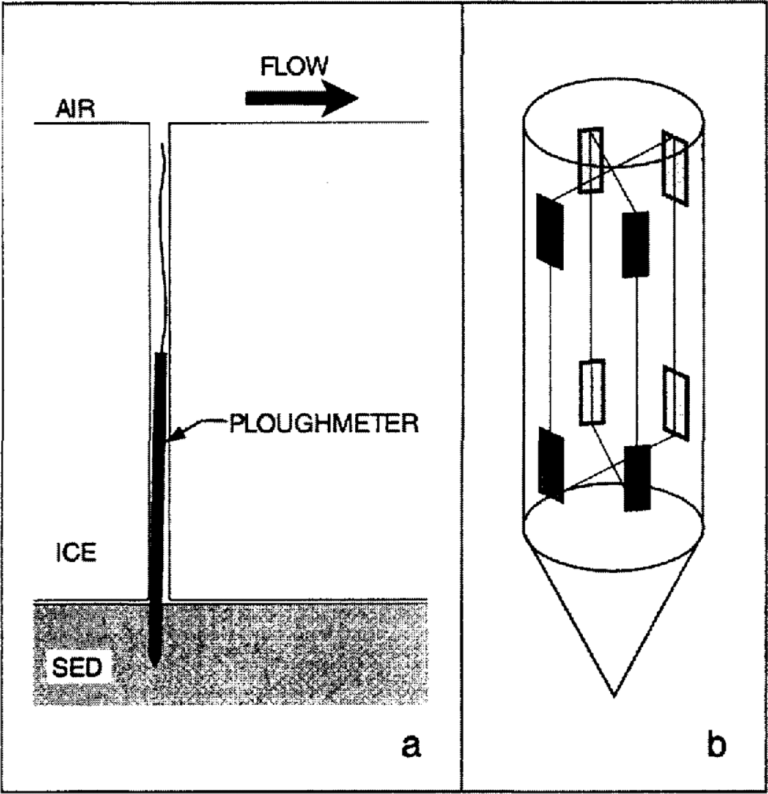
Fig. 1. (a) Schematic diagram of ploughmeter operation. (b) Arrangement of strain gauges near the tip of the steel rod.
In this paper, we interpret data from two ploughmeters and a water-pressure sensor. To support this interpretation we develop a mathematical model to describe the sliding motion of glacier ice over a flat surface having spatially and temporally variable drag. Solving for the velocity field of the ice immediately above the glacier bed, we calculate the behaviour of ploughmeters as they respond to temporal and spatial evolution of basal resistance. Comparison of our model results with field measurements yields evidence for temporal and spatial variations of sticky spots that are linked to changes in basal lubrication.
Field Observations
In July 1992, arrays of ploughmeters and subglacial water-pressure transducers were installed beneath Trapridge Glacier, Yukon Territory, Canada. Figure 2 shows 15 days of observations for ploughmeters 92PL02 and 92PL05. Data from subglacial water-pressure sensor 92P06 are also included and plotted along the same time axis. All three instruments are located within a circle of diameter ~10 m in our main study region near the centre-line flow markers and about 600 m up-flow from the bulge. For a detailed description of the location and setting of the Trapridge Glacier study area see Reference Clarke and Blake.Clarke and Blake (1991). While many of the boreholes drilled to the bed in this region of the glacier were not connected to the subglacial drainage system, obvious communication existed between the holes instrumented with the two ploughmeters and the pressure sensor and the basal hydrological system. The insertion sites of the ploughmeters 92PL02 and 92PL05 were approximately 10 m apart and the line joining the two sites was at an angle of ~8° from the direction of glacier flow.

Fig. 2. Data from ploughmeters and pressure sensor. (a) Force record indicating force applied to the tip of ploughmeter 92PL02. (b) Azimuth of the forces with respect to the internal coordinates of 92PL02. (c) Force record indicating force applied to the tip of ploughmeter 92PL05. (d) Azimuth of the forces with respect to the internal coordinates of 92PL05. (e) Subglacial water-pressure record from pressure sensor 92P06. Super- flotation pressures correspond to a water level if more than about 63 m.
The records of both ploughmeters (Fig. 2a–d) display strong diurnal signals which appear to be correlated with large and rapid fluctuations in subglacial water pressure indicated by sensor 92P06 (Fig. 2c). This correlation suggests that mechanical conditions at the bed vary temporally in response to changes in the basal hydrological system. However, there is a conspicuous difference in how the two ploughmeters respond to these changes in basal conditions. In the case of 92PL05 we see that variations in subglacial water pressure (Fig. 2e) are in phase with variations in the force response (Fig. 2a): high and low water pressures correspond to high and low forces, respectively. In fact, for the time period starting 21 July, the two records look virtually identical, even to the finest detail. In contrast, peak water pressures appear to coincide with low forces experienced by 92PL02 and vice versa (Fig. 2c and c). Thus, comparing Figure 2a and c, we observe that the force record of 92PL05 indicates a response that is 180° out-of-phase with respect to that of 92PL02. At the same time, however, the azimuth records (Fig. 2b and d) indicate ploughmeter responses that are in phase with each other: for both ploughmeters the force angle appears to be rotating in the same sense back and forth by roughly 10°. This force-angle rotation might result from localized and temporally varying changes in the direction of glacier flow.
Qualitative Interpretation
The correlation between the azimuth responses together with the strong anticorrelation between the force responses of the two ploughmeters could suggest that both ploughmeters are responding to the same external forcing. In the following analysis, we investigate the possibility that the mechanical behaviour of both ploughmeters is forced by variations in subglacial water pressure by a mechanism that operates differently for the two ploughmeters.
Reference Fischer and Clarke.Fischer and Clarke (1994) showed that if subglacial sediment is treated as a layer of Newtonian viscous fluid, then the force on a ploughmeter that is moving through it is linearly proportional to the effective fluid viscosity μ, the translational velocity ν and a geometrical factor dependent on the shape and dimensions of the section of ploughmeter immersed in sediment (see Reference Fischer and Clarke.Fischer and Clarke, 1994, Equation (9)). The translational velocity ν is equal to the basal glacier sliding velocity ν b if subglacial sediment deformation is neglected. Thus, variations in the force response of a ploughmeter could be due to any or all of the following: changes in the strength of basal material, changes in glacier sliding rate and changes in ploughmeter insertion depth into subglacial sediment. As in our previous analysis (Reference Fischer and Clarke.Fischer and Clarke, 1994), we attribute all the variations in the force response to changes in basal sliding rate rather than changes in the insertion depth or strength of basal sediments.
Measurements of water pressure beneath Trapridge Glacier show that at any given time, basal water pressure is not uniform over the glacier bed (Reference Stone and Clarke.Stone and Clarke, 1996). In addition, large spatial pressure gradients can be observed between boreholes that are connected and those that are unconnected to the subglacial drainage system (Reference Murray and Clarke.Murray and Clarke, 1995). These observations suggest that we must treat mechanical conditions at the glacier bed on a local scale and that mechanical conditions should vary in response to localized changes in the subglacial hydrological system. In the following, we base our interpretation on the idea that a lubricating water film is associated with high subglacial water pressure, which effectively decouples the glacier from its bed and promotes sliding. In contrast, low pressures cause increased bottom drag. This idea follows from theory and observation that in a distributed subglacial drainage system, ice–bed separation by water increases with water pressure and that the glacier sliding velocity increases with ice–bed separation (Reference AlleyAlley, 1996; and references therein). Significantly, measurements of bed deformation, bed shear strength, subglacial water pressure and surface speed at Storglaciaren, Sweden (Reference Iverson, Hanson., Hooke. and Jansson.Iverson and others, 1995; Reference Hooke., Hanson., Iverson, Jansson. and Fischer.Hooke and others, 1997), showed that the shear-strain rates of the bed decrease during periods of high water pressure and increased surface flow rate. Elevated water pressures were therefore inferred to weaken the coupling of ice with the bed, allowing the glacier to move over the bed faster while deforming it less rapidly. This inference is substantiated by continuous measurements of basal sliding and subglacial water pressure at Trapridge Glacier (Reference Blake, Fischer. and Clarke.Blake and others, 1994; Reference Fischer and Clarke.Fischer and Clarke, 1997) which indicated that there is substantial motion at the glacier sole during periods of rising water pressure.
We consider a patch of glacier bed over which, at a starting time t = t 1 the basal water pressure is low. There is good mechanical coupling between the glacier and the subglacial sediment because bed lubrícation is poor. Basal resistance to sliding is higher than average, and little slip occurs between the bed and the overlying ice (Fig. 3a). At a later time t = t 2, subglacial water pressure has increased over the patch. Now the ice–bed interface is well lubricated and there is strong local decoupling of the glacier from its bed. Ice can slide more easily over this patch having lower than average bottom drag (Fig. 3b). As water pressure rises on the patch of bed under consideration, some of the shear traction exerted by the overlying ice will be redistributed onto surrounding regions.

Fig. 3. Schematic diagram of temporal evolution of ice flow as a function of basal resistance. Shaded areas represent regions having higher than average bottom drag, while white areas indicate lower than average drag. (a) Low subglacial water pressure in centre of diagram. (b) High subglacial water pressure in centre of diagram.
While this interpretation ensures a roughly constant mean basal resistance averaged over the glacier bed, it also allows for spatially and temporally varying bottom drag as sticky spots are created and destroyed in response to fluctuations in subglacial water pressure. If a ploughmeter was positioned within the “sticky/slippery” patch in Figure 3 and another in the surrounding region, we see that the two ploughmeters would respond to the diurnal water-pressure forcing in ways that were 180° out-of-phase with respect to each other.
Quantitative Interpretation
The foregoing qualitative explanation of water-pressure effects on bed coupling leads us to a mathematical treatment of ice flow over a bed having varying basal resistance to sliding. In this section we compute the velocity field for the ice immediately above the glacier bed as a function of bottom drag and explore how ploughmeters respond to the creation and destruction of sticky spots. In our model, we treat the bed as a hard, flat surface over which glacier sliding is controlled by spatially and temporally varying drag at the ice–bed interface. We note that we neglect the possible softening influence of high subglacial water pressures on the strength of the sedimentary bed. We make this assumption solely for the purpose of the model, but we appreciate that it is likely to be an oversimplification.
Physical model and outline of analysis
We analyze the flow of ice for a configuration in which the glacier is treated as a planar parallel-sided slab of linear viscous rheology that rests on an incline. Coordinates are chosen with the x axis along the ice–bed interface directed in the glacier flow direction and the z axis normal to the bed and pointed positive upward.
The problem is formulated as follows. For glacier ice treated as a linear viscous fluid with constant density ρ I and constant viscosity η and flowing at velocities slow enough that inertial effects can be neglected, the ice-flow velocity field v satisfies
where η is the dynamic viscosity of ice, g is the acceleration due to gravity and p is the pressure within the fluid. Ice is taken to be incompressible, thus
We further assume that the inclined bed is a “flat” surface with a variable drag coefficient f over which the ice moves with variable basal sliding velocity vb These assumptions contrast with those of standard glacier sliding theories where ice overlies a bedrock surface having a given topography and resistance arises from interaction of the ice with roughness elements. Here, the variability in the resistance to sliding is caused by patches of higher than average basal drag. The origin of the drag is the absence of a lubricating water film at the ice–bed interface during periods of low basal water pressures. Ice responds to the increased drag on the upstream sides of sticky patches by slowing down and diverging laterally at these points, thereby permitting the ice to move forward. Correspondingly, it speeds up and converges behind the sticky spots, in response to the reduced drag on the downstream sides. We assume that the basal shear traction vector Tb is linearly proportional to the basal sliding rate
where f is a drag coefficient. Equation (3) is in direct analogy to the approach taken by Reference MacAyealMacAyeal (1992) in his calculation to infer basal friction from the observed surface velocity pattern of Ice Stream E.
First-order perturbation
We consider the drag coefficient f to consist of a spatially-constant background component f 0, which could be a function of time, upon which is superimposed a perturbation component f ′ which varies with time and position across the glacier bed. Hence,
with the condition that (f ′ (x,y,t)) = 0, where the angled brackets denote averaging over the glacier bed. With this assumption we note that the ice-flow velocity field is also the sum of a slowly varying background component and a more rapidly varying perturbation component, i.e.
Similarly, we can write for the basal sliding velocity vb that
where ![]() and
and ![]() . Substituting Equations (4) and (6) into Equation (3) and ignoring higher-order perturbation terms yields
. Substituting Equations (4) and (6) into Equation (3) and ignoring higher-order perturbation terms yields

We can split Equation (7) into two equations, one that represents linear background sliding,
and one that describes linear sliding due to the perturbation effects,
Note that in Equation (7), Tb varies with both time and space but its variations are constrained by the fact that the average over the glacier bed ![]() . Likewise in Equation (9) the spatial average of the perturbation
. Likewise in Equation (9) the spatial average of the perturbation ![]() vanishes. Equation (4) further implies that the pressure also consists of a temporally and spatially varying perturbation component superimposed onto a time-varying background component, i.e.
vanishes. Equation (4) further implies that the pressure also consists of a temporally and spatially varying perturbation component superimposed onto a time-varying background component, i.e.
Finally we make the simplifying assumption that the coordinate system is aligned with the background sliding component which is oriented along the positive x axis; thus ![]() and
and ![]() , where i and j are unit vectors.
, where i and j are unit vectors.
Variations in sliding due to perturbation effects
Substitution of Equations (5) and (10) into Equation (1) gives
The linearity of Equation (11) results in the perturbation fields being independent of and additional to the background distribution. Hence, the perturbation equations that command attention are the following:
and
Equation (13) is equivalent to the incompressibility equation and follows from taking the divergence of Equation (12) and imposing the condition ![]() (Equation (2) ). The gravitational body force does not appear in Equation (12) because perturbation effects are not driven by gravity.
(Equation (2) ). The gravitational body force does not appear in Equation (12) because perturbation effects are not driven by gravity.
We follow the treatment used by Reference KambKamb (1970) on regelation sliding and solve Equations (12) and (13) by the Fourier-analytical method. Fourier transformation of Equation (13) with respect to x and y gives

If one assumes that the surface is very far from the bed then the standard solution of Equation (14) is
The boundary conditions that are satisfied by Equation (15) are that the pressure perturbations at the bed (where z = 0) are described by ![]() and that the perturbations vanish as z becomes large.
and that the perturbations vanish as z becomes large.
In a similar fashion the three components of the Fourier-transformed version of Equation (12) can be written as


where ![]() . Equations (16a–c) have the general form
. Equations (16a–c) have the general form
and the general solution
Applying Equation (18) to the solution of Equations (16a–c) gives the solutions


The incompressibility condition (Equation (2)) requires that

and applying this condition imposes restrictions on Equation (19a–c). Performing this step gives

Equation (21) can be applied to the velocity solutions Equation (19a–c) to obtain


Now we relate perturbations in basal stress to those of basal velocity. From the constitutive equation for a linear viscous fluid
where σ ij is the stress tensor,![]() is the strain-rate tensor and δ ij is the Kronecker delta, it follows that
is the strain-rate tensor and δ ij is the Kronecker delta, it follows that
with similar equations applying to the perturbation stress and velocity fields. In Fourier-transformed variables the equations of interest are


From Equations (22a) and (22b) it follows that


At the z = 0 boundary the friction law (Equation (9)) gives the following relationships:
In Equation (27b) we assumed that the coordinate system has been chosen such that ![]() . Combining Equations (26) and (27) we find that
. Combining Equations (26) and (27) we find that

Note that Equations (28a) and (28b) constitute a pair of linear equations in the unknowns ![]() and
and ![]() . From Equation (28b) it is apparent that the y component of the perturbation velocity field is
. From Equation (28b) it is apparent that the y component of the perturbation velocity field is
Substituting Equation (29) into Equation (28a) and solving for ![]() gives the x component of the perturbation velocity field
gives the x component of the perturbation velocity field

Description of drag-coefficient surface
Consider a part of the bed of area A, assumed to be rectangular of dimensions L x and L y in the x and y directions. Within this area we define a drag-coefficient surface f(x, y, t) to consist of a spatially constant background component f 0(t) superimposed by a spatially and temporally variable perturbation component f ′ (x, y, t) with the condition that
where the angled brackets denote averaging over A (Fig. 4). The perturbation drag-coefficient surface is described by patches with dimensions w x and w y in the x and y directions, respectively, that are centred on coordinates ![]() and have higher than average drag
and have higher than average drag ![]() , while a lower than average drag
, while a lower than average drag ![]() has been assigned to the rest of the surface. The magnitude of
has been assigned to the rest of the surface. The magnitude of ![]() cannot exceed f 0(t) since a negative drag coefficient f(x,y,t) is not physically meaningful. In addition, the magnitudes of
cannot exceed f 0(t) since a negative drag coefficient f(x,y,t) is not physically meaningful. In addition, the magnitudes of ![]() and
and ![]() are generally not equal and depend on the areal fraction that is covered by sticky patches (e.g. small patches with large positive
are generally not equal and depend on the areal fraction that is covered by sticky patches (e.g. small patches with large positive ![]() values are accompanied by small negative
values are accompanied by small negative ![]() values for the rest of the surface).
values for the rest of the surface).

Fig. 4. Diagram of drag-coefficient surface f(x, y, t) defined over a rectangular region of area A = L x L y.
We take the drag-coefficient surface f(x, y, t) to be periodically repeated over the entire x-y plane, so that the bed, of assumed infinite extent, consists of a checkerboard of identical areas A, across which the ice slides in the x direction. While a real glacier bed is not periodic in this strict sense, our assumption of repeat distances L x and L y simplifies calculation of the Fourier transform of the perturbation drag-coefficient surface.
Model results
In Table 1 we have listed the model parameters that were used to obtain the calculated solutions. Glen’s flow law combined with Equation (23) yields an estimate of the effective dynamic viscosity of ice

where ![]() is the basal shear-stress magnitude. Using a flow-law parameter for temperate ice (B = 6.8 × 10⁻¹⁵ s−1 kPa−3, n = 3 (Reference PatersonPaterson, 1994, p.97)) and a mean basal shear stress of τ b = 77 kPa (based on an ice-thickness of 72 m and a surface slope of 7°), we calculated a Trapridge Glacier ice viscosity of η = 1.24 × 10¹³ Pa s. Enhanced creep due to stress concentrations near the bed is likely to soften this basal ice; thus, we reduce the value of ice viscosity by one order of magnitude and, somewhat arbitrarily, take η = 3.0 × 10¹² Pa s in our model calculations (Table 1). With an average basal sliding velocity for Trapridge Glacier of
is the basal shear-stress magnitude. Using a flow-law parameter for temperate ice (B = 6.8 × 10⁻¹⁵ s−1 kPa−3, n = 3 (Reference PatersonPaterson, 1994, p.97)) and a mean basal shear stress of τ b = 77 kPa (based on an ice-thickness of 72 m and a surface slope of 7°), we calculated a Trapridge Glacier ice viscosity of η = 1.24 × 10¹³ Pa s. Enhanced creep due to stress concentrations near the bed is likely to soften this basal ice; thus, we reduce the value of ice viscosity by one order of magnitude and, somewhat arbitrarily, take η = 3.0 × 10¹² Pa s in our model calculations (Table 1). With an average basal sliding velocity for Trapridge Glacier of ![]() (Reference Blake, Fischer. and Clarke.Blake and others, 1994) substituted into Equation (8) the resulting background drag coefficient is f 0 = 1.66 × 10¹¹ Pa s m−1 (Table 1).
(Reference Blake, Fischer. and Clarke.Blake and others, 1994) substituted into Equation (8) the resulting background drag coefficient is f 0 = 1.66 × 10¹¹ Pa s m−1 (Table 1).
Table 1. Parameters for “sticky spot” model

For the model calculations discussed in this section, area A has been divided into a 32 × 32 grid. Following the description in the previous section, positive ![]() or negative
or negative ![]() values were then assigned to every gridpoint. The frictional perturbation f ′(x, y, t) was Fourier-transformed using a two-dimensional fast-Fourier-transform algorithm (Reference Press, Teukolsky., Vetterling. and Flannery.Press and others, 1992, p. 515) to obtain
values were then assigned to every gridpoint. The frictional perturbation f ′(x, y, t) was Fourier-transformed using a two-dimensional fast-Fourier-transform algorithm (Reference Press, Teukolsky., Vetterling. and Flannery.Press and others, 1992, p. 515) to obtain ![]() and subsequently substituted into Equation (30) to find the sliding velocity perturbation
and subsequently substituted into Equation (30) to find the sliding velocity perturbation ![]() . The sliding perturbation
. The sliding perturbation ![]() follows immediately from Equation (29). Inverse Fourier transformation of the perturbation velocity field
follows immediately from Equation (29). Inverse Fourier transformation of the perturbation velocity field ![]() yields v ′ (x, y, 0, t).
yields v ′ (x, y, 0, t).
The drag-coefficient surface shown in Figure 5a consists of rectangular patches having higher than average drag centred on gridpoint (17, 17) and the four corners of area A, while the remainder of A has lower than average drag. For a peak perturbation drag coefficient ![]() for the patches having dimensions w x = 16 and w y = 6 gridpoints, we obtained
for the patches having dimensions w x = 16 and w y = 6 gridpoints, we obtained ![]() for the rest of the surface from Equation (31). The resulting flow velocity field (Fig. 5b) shows how the ice is being slowed down and diverted around the high-resistance patch in the centre of area A. Here and in subsequent plots of flow velocity fields, the background sliding velocity
for the rest of the surface from Equation (31). The resulting flow velocity field (Fig. 5b) shows how the ice is being slowed down and diverted around the high-resistance patch in the centre of area A. Here and in subsequent plots of flow velocity fields, the background sliding velocity ![]() has been added to the perturbation velocity field (note that
has been added to the perturbation velocity field (note that ![]() ). In Figure 5c, the drag-coefficient surface consists of a resistance low in the centre of area A with patches of higher than average drag located on the midpoints of the sides of the square area. Now the ice is allowed to accelerate and be channelled toward this low-resistance patch (Fig. 5d).
). In Figure 5c, the drag-coefficient surface consists of a resistance low in the centre of area A with patches of higher than average drag located on the midpoints of the sides of the square area. Now the ice is allowed to accelerate and be channelled toward this low-resistance patch (Fig. 5d).

Fig. 5. Drag-coefficient surfaces, as defined on a 32 × 32 grid of area A, and calculated ice-flow velocity fields immediately above the glacier bed. (a) High drag centred on gridpoint (17, 17). (b) Divergent and slowed-down ice flow, (c) Low drag in the centre of area A. (d) Convergent and accelerated ice flow. The locations of two numerical ploughmeters (PL1 and PL2) positioned at gridpoints (7, 16) and (23, 18) are also indicated.
Figure 5b and d show that, as the central region of A alternates between being sticky and slippery, some of the flow vectors rotate back and forth and change their lengths. The change in length of a flow vector corresponds to a change in basal sliding velocity of ice at that point, whereas rotation indicates a reorientation of the ice-flow direction. For patchiness length scales substantially less than the ice thickness there is a negligible response at the glacier surface to such variations in the pattern of the basal sliding velocity (Reference Balise and Raymond.Balise and Raymond, 1985). If one accepts that variations in the force response of a ploughmeter indicate changes in the sliding velocity caused by temporal and spatial variations of basal resistance, it follows that for Trapridge Glacier the basal resistance is highly variable over distances of O(10) and sub-daily time-scales. This variability is attributed to changes in the subglacial hydrological system, an interpretation that is strengthened by the findings of Reference Murray and Clarke.Murray and Clarke (1995) and Reference Stone and Clarke.Stone and Clarke (1996) who show that over short distances the subglacial water system is highly heterogeneous and that rapid pressure changes can occur at the bed. Because of the short time-scale for creation and destruction of sticky spots, significant changes in glacier geometry cannot develop and a quasi-static assumption is justified.
We now consider how ploughmeters might respond to the diurnal creation and destruction of sticky spots. In our further analysis, we imagine the consequence of positioning two ploughmeters (PL1 and PL2) at gridpoints (7, 16) and (23, 18) (Fig. 5). With the side lengths of area A chosen to be L x = L y = 20 m, the location of these gridpoints corresponds to a separation of the ploughmeters by approximately 10 m, while the line joining the two points forms an angle of ~7° with the x direction. This choice of ploughmeter positioning is therefore consistent with the known properties of the field set-up (the insertion sites of ploughmeters 92PL02 and 92PL05 were ~10 m apart, while the line joining the sites was at an angle of ~8° from the direction of glacier flow). With our assumption that the force response of a ploughmeter is linearly proportional to the basal sliding rate, we note that the change in length of the flow vectors at the two gridpoints translates into a change in forces experienced by PL1 and PL2. In addition, the rotation of the flow vectors is equivalent to a rotation of the force angle about the ploughmeters.
Recalling our assumption of a water-pressure-dependent basal resistance to sliding, we computed the force and azimuth responses of PL1 and PL2 (Fig. 6) for a varying basal drag that is based on the water-pressure record shown in Figure 2e. In our calculations, low subglacial water pressures correspond to high resistance in the centre of area A and vice versa. The force responses shown in Figure 6a and c) are normalized with respect to the background basal sliding velocity ![]() . The computed results (Fig. 6) display a striking similarity to the field data shown in Figure 2: the force records (Fig. 6a and c) indicate variations that are 180° out-of-phase with each other, while the azimuth records (Fig. 6b and d) show an in-phase rotation of the force angle by roughly 10°.
. The computed results (Fig. 6) display a striking similarity to the field data shown in Figure 2: the force records (Fig. 6a and c) indicate variations that are 180° out-of-phase with each other, while the azimuth records (Fig. 6b and d) show an in-phase rotation of the force angle by roughly 10°.
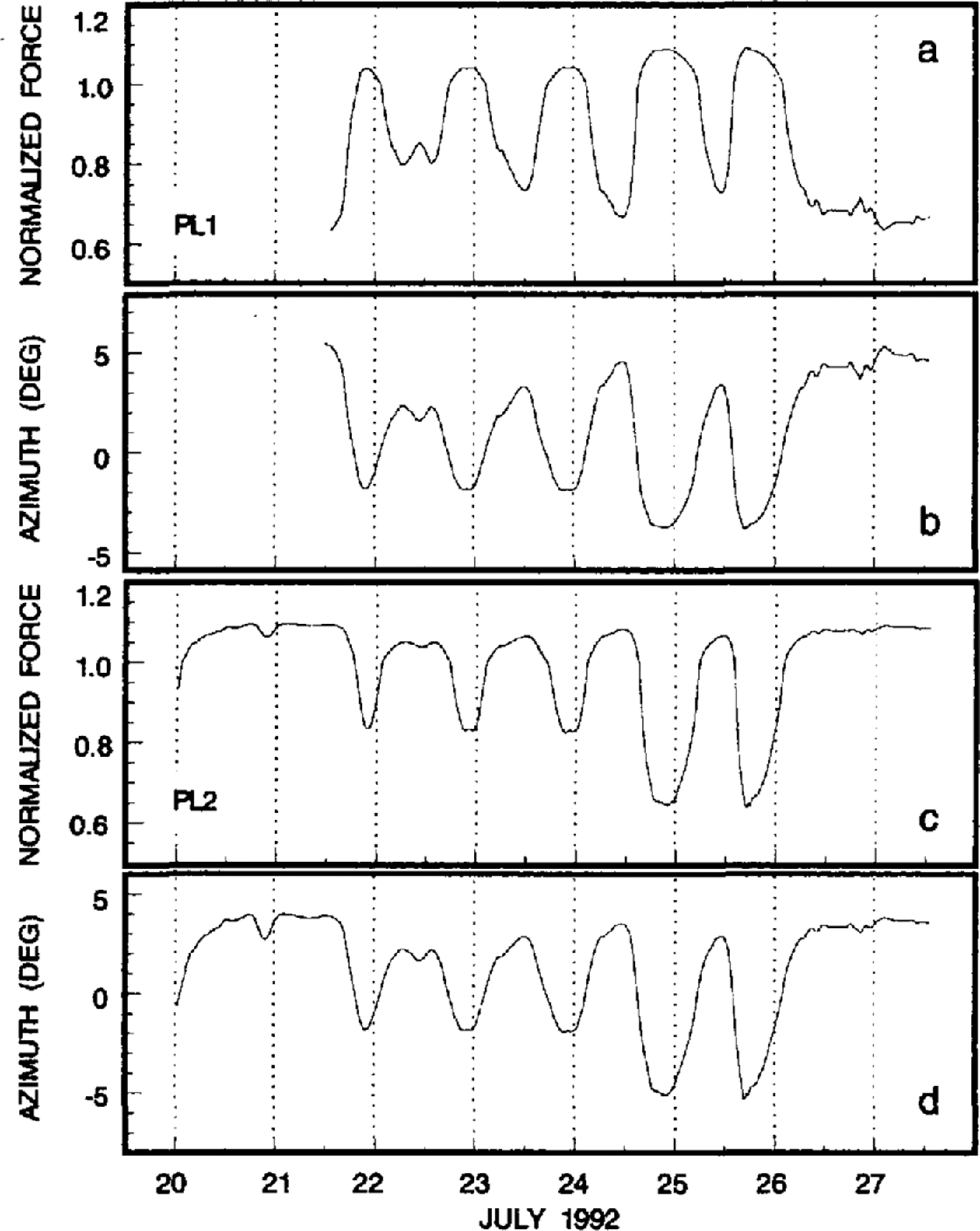
Fig. 6. Computed responses of two numerical ploughmeters (PL1 and PL2) positioned at gridpoints (7, 16) and (23, 18) for a varying basal drag that is based on the water-pressure record shown in Figure 2e. (a) Synthetically generated force record for PL1. (b) Synthetically generated azimuth record for PL1. (c) Synthetically generated force record for PL2. (d) Synthetically generated azimuth record for PL2. Note the similarity to Figure 2a–d.
Concluding Discussion
Our model calculations for the flow of ice over a flat surface having variable resistance are based on the approximation that ice behaves as a linear viscous fluid. The purpose of the model is to demonstrate how local values of shear stress might vary with time and space. The non-linearity of Glen’s flow law would greatly complicate the model without contributing additional insight.
In our derivation of Equation (9), we neglected higher-order perturbation terms. This is an acceptable approximation when perturbations of the drag coefficient are small compared to the background drag coefficient. However, from Table 1 we see that the coefficients for background drag and perturbation drag have values that are of the same order of magnitude. Thus our model can be faulted for using a linear perturbation analysis to describe a situation where the neglected non-linear terms may be quite large. In this respect the present work shares a shortcoming common to all glaciological exploitations of linear sliding theory. Nevertheless, a more rigorous analysis which retained these non-linear terms should also attend to the other expedient assumptions of our model, namely, linear ice rheology and a highly simplified sliding law.
A possible incongruity of our model relates to the comparative stiffness of ice and subglacial material. Implicitly we assume that the bed is typically soft enough to allow ploughmeters to be dragged through it, yet locally stiff enough to resist and deflect the flow of overlying ice. An alternative model, antithetical to ours, might also yield a consistent explanation of the ploughmeter records (Fig. 2). If, in comparison with bed material, ice was assumed to be essentially rigid, then the deformation response to patchy-stickiness at the ice bed contact would be concentrated in the bed and there would be no deflection of the ice flow. Anomalous signals from the ploughmeters would then be taken as indications of sediment motion rather than ice motion. It might be possible to develop an interpretation model that would, for a linear viscous till rheology, resemble the mirror image ofthat described in the present paper. We cannot discount this possibility, but have reasons to prefer the view that ice is deformable and responsive to local concentrations of sliding resistance. Icequakes, numerous throughout the summer melt season, and deep englacial cracks, encountered during hot-water drilling, are clear evidence for the existence of large deviatoric stresses near the glacier bed. A uniformly weak substrate would be incapable of transmitting such stresses into the overlying ice. In a previous paper (Reference Fischer and Clarke.Fischer and Clarke, 1994) our interpretation of ploughmeter records assumed a linear viscous till rheology, but this is clearly an oversimplification. Subglacial sediments tend to be highly heterogeneous and span a wide range of grain-sizes. This characteristic might result in scale-dependent rheological properties that could reconcile the conflicting requirements of soft-bed interactions with ploughmeters and hard-bed interactions over large sticky spots.
In conclusion, our observations and model calculations point to the existence of sticky spots beneath Trapridge Glacier. Although we have demonstrated consistency for only one example, it is conceivable that there are sticky spots all across the bed of our main study region. These sites of enhanced basal drag are ephemeral in nature because they are created and destroyed in response to fluctuations in subglacial water pressure. Therefore, it is unlikely that they support a large fraction of the driving stress for ice flow. Our previous result, that the deformational resistance of the sedimentary bed is of comparable magnitude to that required to balance the applied basal shear stress (Reference Fischer and Clarke.Fischer and Clarke, 1994), strengthens our argument that sticky spots are probably not dominant in controlling the flow of Trapridge Glacier.
Our findings can be compared with results from other sites. Interpretation of data collected near the Upstream B camp (Reference AlleyAlley, 1993) suggests that the lubricated regions of the bed support >87% of the basal shear force. This leaves 13% of the basal shear force to be supported on sticky spots, implying that sticky spots do not dominate the force balance in this region of Ice Stream B. However, a study by Reference Echelmeyer, Harrison., Larsen. and Mitchell.Echelmeyer and others (1994) suggests that care has to be taken in extrapolating localized basal conditions in the vicinity of Upstream B camp to the remainder of Ice Stream B. Flow-model calculations indicate that the margins play an important role in controlling ice-stream motion, with marginal drag being equal to or greater than basal drag at some locations. These findings are strengthened by measurements of the marginal shear stress of Ice Stream C which imply that 63 100% of the ice stream’s support against the gravitational driving stress comes from the margins (Reference Jackson and Kamb.Jackson and Kamb, 1997). In contrast to our results, Reference Whillans, Chen., van der Veen and Hughes.Whillans and others (1989) reported that Byrd Glacier, Antarctica, is held mainly by basal drag that is concentrated at a few sites separated by about 13 km. Analysis of work done on Ice Stream C (Reference Alley, Anandakrishnan., Bentley. and Lord.Alley and others, 1994; Reference Anandakrishnan and Alley.Anandakrishnan and Alley, 1994) indicated that the base of the ice stream consists of a weak till interspersed with sticky spots of area on the order of 102 m2 with a spatial density on the order of 10 km−2. As a result of a reduced water lubrication, it is claimed that these sticky spots support almost all of the driving stress and account for the negligible flow of Ice Stream C. Similarly, the basal-friction distribution derived from surface velocity data of Ice Stream E (Reference MacAyeal, Bindschadler. and Scambos.MacAyeal and others, 1995) confirms the suggestion that basal shear stress of the ice stream is extremely low except in isolated sticky spots. These sticky spots where basal friction exceeds the area-averaged driving stress are inferred to be scattered irregularly across the subglacial regime and comprise approximately 15% of the ice-stream area.
Acknowledgements
We thank the Natural Sciences and Engineering Research Council of Canada for funding this study, and the University of British Columbia for providing postgraduate fellowship support. Our fieldwork was conducted in Kluane National Park. We thank Parks Canada and the Government of the Yukon Territory for granting permission to carry out studies in the park. Advice and assistance during our field program were gratefully received from S. J. Marshall, T. Murray and B. S. Waddington. We further acknowledge C. F. Raymond, R. B. Alley and W. D. Harrison for valuable comments and criticisms.


