


Introduction
Extensive supraglacial debris mantle on the ablation zone modifies glacier response to climate forcing (Scherler and others, Reference Scherler, Bookhagen and Strecker2011a; Nuimura and others, Reference Nuimura, Fujita, Yamaguchi and Sharma2012; Banerjee and Shankar, Reference Banerjee and Shankar2013; Gardelle and others, Reference Gardelle, Berthier, Arnaud and Kaab2013; Brun and others, Reference Brun, Berthier, Wagnon, Kääb and Treichler2017; King and others, Reference King, Dehecq, Quincey and Carrivick2018). The supraglacial debris layer mediates the melt-energy supply to the ice-surface underneath. A thick debris layer inhibits melt by insulating the ice, whereas a thin-debris layer increases melt due to a lower albedo (Østrem, Reference Østrem1959; Collier and others, Reference Collier2014). However, in the limit of a very thin debris layer ($\lesssim\!\!2$ cm), increased evaporation reduces the energy available for melting (Collier and others, Reference Collier2014) leading to a decline in ablation (Østrem, Reference Østrem1959). Supraglacial debris advects with the ice flow, and the debris layer generally thickens down-glacier as the ice velocity declines (Benn and Lehmkuhl, Reference Benn and Lehmkuhl2000; Kirkbride and Deline, Reference Kirkbride and Deline2013; Anderson and Anderson, Reference Anderson and Anderson2016). This thickening of debris layer causes a systematic reduction in ablation rate down-glacier, even though elevation decreases. This is in contrast with the down-glacier increase in ablation which is typically seen on debris-free glaciers (e.g., Oerlemans, Reference Oerlemans2001). The resultant inverted mass-balance profile on the debris-covered ablation zone has profound implications on the evolution of a glacier under a warming climate (Banerjee and Shankar, Reference Banerjee and Shankar2013). The most striking feature of which is a decoupling of length and mass changes of the glacier right after the warming starts: a thickly debris-covered glacier initially loses mass mostly by thinning, even as its length remains steady over a period of stagnation that may span several decades (Naito and others, Reference Naito, Nakawo, Kadota and Raymond2000; Banerjee and Shankar, Reference Banerjee and Shankar2013). A combination of a slow evolution of the ice-flux patterns under the climate forcing and low melt rates beneath the debris cover are responsible for the formation of the stagnant tongue. Beyond this the period of stagnation, a relatively high net mass-loss rate is expected on debris-covered glaciers (Banerjee, Reference Banerjee2017). With an extensive supraglacial debris cover over 40% of the total ice mass in the ablation zones of several regions in the Himalaya-Karakoram (Kraaijenbrink and others, Reference Kraaijenbrink, Bierkens, Lutz and Immerzeel2017), the above-mentioned debris effects have left strong imprints in the recent ice-loss pattern in the Himalaya (Scherler and others, Reference Scherler, Bookhagen and Strecker2011a; Nuimura and others, Reference Nuimura, Fujita, Yamaguchi and Sharma2012; Banerjee and Shankar, Reference Banerjee and Shankar2013; Gardelle and others, Reference Gardelle, Berthier, Arnaud and Kaab2013; Brun and others, Reference Brun, Berthier, Wagnon, Kääb and Treichler2017; King and others, Reference King, Dehecq, Quincey and Carrivick2018) and may crucially impact its future evolution as well (Kraaijenbrink and others, Reference Kraaijenbrink, Bierkens, Lutz and Immerzeel2017).
The smooth down-glacier increase in debris thickness, and the corresponding decline of the surface ablation rate as discussed above, provide only a first- order description of the debris effects (Benn and Lehmkuhl, Reference Benn and Lehmkuhl2000; Scherler and others, Reference Scherler, Bookhagen and Strecker2011b; Banerjee and Shankar, Reference Banerjee and Shankar2013). The role of several other complicating factors, e.g., the presence of numerous thermokarst ephemeral ponds and cliffs that increase local melt rate (Reynolds, Reference Reynolds2000; Sakai and others, Reference Sakai, Takeuchi, Fujita and Nakawo2000; Miles and others, Reference Miles, Willis, Arnold, Steiner and Pellicciotti2017), vertical and horizontal variations of the thermal properties of debris (Nicholson and Benn, Reference Nicholson and Benn2013; Rowan and others, Reference Rowan2017), the random short-scale spatial variation of debris thickness (Mihalcea and others, Reference Mihalcea2006; Zhang and others, Reference Zhang, Fujita, Liu, Liu and Nuimura2011; Nicholson and Mertes, Reference Nicholson and Mertes2017; Rounce and others, Reference Rounce, King, McCarthy, Shean and Salerno2018) and the accumulation contribution from avalanches (Laha and others, Reference Laha2017) need to be quantified for accurate surface mass-balance estimates on any typical debris-covered Himalayan glacier. The standard glaciological mass-balance measurement protocol (Kaser and others, Reference Kaser, Fountain and Jansson2003) may not be designed to handle the above issues. Among the complications listed above, the random spatial fluctuation of supraglacial debris thickness, and its implication on glacier mass balance have been highlighted only recently (Nicholson and others, Reference Nicholson, McCarthy, Pritchard and Willis2018). The variability of sub-debris ablation rate due to a spatially fluctuating debris thickness is likely to be a significant limiting factor for the accuracy of glaciological mass-balance measurements on debris-covered glaciers, as the estimation of glacier-wide mean specific ablation from observations at a finite set of stakes assumes that ablation rate is determined solely by elevation (Cogley, Reference Cogley1999).
In this paper, field data from the debris-covered Satopanth Glacier (Central Himalaya, India) are used to investigate the effects of spatial fluctuations of debris thickness on the accuracy of glaciological mass-balance estimates. An alternative protocol for mass-balance estimation over the debris-covered ablation zone is proposed and tested. We analyse ~1100 approximately bi-weekly measurements of ablation rate at a network of up to 56 bamboo stakes over the ablation seasons of 2015, 2016 and 2017. Debris-thickness data from 191 pits dug on the glacier surface are used to study the debris-thickness distribution. We interpolate the observed point-scale ablation rates as a function of (I) elevation and (II) debris thickness at the stakes. The interpolated values for each of the measurement periods are then averaged over glacier hypsometry (method-I, the standard glaciological method) and the zonal debris-thickness distribution (method-II), respectively, to obtain two estimates of the total ablation over the debris-covered area. The reliability of both the regression methods is quantified, the estimated mean sub-debris ablation obtained from both the methods is compared, and corresponding uncertainties in the estimates are analysed. Possible biases in the ablation estimates as a function of the number of stakes used are investigated for both the methods.
Glaciological mass-balance measurement and debris cover
Glaciological mass-balance estimation is one of the most basic and fundamental tools in glaciology. This relatively simple and robust method estimates the mean specific mass balance of a glacier using observations of ablation and accumulation rates at a network of relatively small ($\sim\!\! 5\!\!-\!\!15$ ) number of stakes/pits (Fountain and Vecchia, Reference Fountain and Vecchia1999; Kaser and others, Reference Kaser, Fountain and Jansson2003). In one of the prescribed procedures (Kaser and others, Reference Kaser, Fountain and Jansson2003), the stake data are fitted to a quadratic curve as a function of elevation, and then averaged over the corresponding area-elevation distribution (Kaser and others, Reference Kaser, Fountain and Jansson2003) to obtain the mean ablation. Interestingly, the number of stakes required is largely independent of the size of the glacier as long as its area is ≲10 km2 (Fountain and Vecchia, Reference Fountain and Vecchia1999). The robustness of the method relies upon strongly correlated surface ablation rates at all the locations within the same elevation band (Cogley, Reference Cogley1999). An alternative procedure (Kaser and others, Reference Kaser, Fountain and Jansson2003) involves preparing a contour-map of local mass balance based on the stake data. Here, detailed knowledge of local field conditions could be incorporated to improve the accuracy of the estimate.
The presence of extensive supraglacial debris cover poses several problems for the above glaciological mass-balance estimation method so that the standard mass-balance manual (Kaser and others, Reference Kaser, Fountain and Jansson2003) advises against choosing debris-covered glaciers for glaciological mass-balance measurements: ‘It is most convenient if the glacier is free of debris cover. A debris cover, usually limited to the tongues, complicates the interpretation of the climate- glacier interaction. Besides of this theoretical consideration the installation and maintenance of an ablation network (stakes) is difficult. Even if it was installed, the regular visits to such a stake in the middle of more or less loose boulders of each size is dangerous’ (Kaser and others, Reference Kaser, Fountain and Jansson2003, p. 28). Apart from these practical considerations, a major issue with the standard glaciological method is that it does not take into account the random spatial variability of debris thickness. While supraglacial debris thickness increases systematically down-glacier and thus, may be correlated with elevation on glaciers with simple geometry (Anderson and Anderson, Reference Anderson and Anderson2016), a relatively large local variability of debris thickness is known to be present at any given elevation band (Nicholson and others, Reference Nicholson, McCarthy, Pritchard and Willis2018). This random variability of debris thickness would lead to a corresponding large variability in the ablation rate within each elevation band, so that the data from an individual stake may not reflect the mean ablation in the corresponding elevation band. Moreover, because of the non-linear dependence of ablation rate on debris-thickness (Østrem, Reference Østrem1959), mean debris thickness in an elevation band can not be used to estimate mean melt rate (Nicholson and others, Reference Nicholson, McCarthy, Pritchard and Willis2018). A contour map-based extrapolation of stake data can be more accurate as field knowledge of large-scale debris thickness variation may be incorporated into the calculation. However, the local-scale debris thickness variability discussed above would still be an issue.
For a rough estimate of the magnitude of the effects of debris variability on ablation rate, let us assume the following form for the variation of ablation rate b with debris thickness d (Evatt and others, Reference Evatt2015; Anderson and Anderson, Reference Anderson and Anderson2016),

Here, b 0 is the ablation rate on debris-free ice, and d 0 (~10 cm) is a characteristic debris-thickness scale (Anderson and Anderson, Reference Anderson and Anderson2016). The above formula implies that a possible variation of debris thickness from, say ~10 cm to 1 m can reduce the ablation rate by a factor of about 6. Similar variations in ablation rate for clean ice Himalayan glaciers (with typical mass-balance gradients of ~0.6 m w.e. yr−1 100 m−1) would correspond to an elevation difference of about a thousand meters (Azam and others, Reference Azam2018). Therefore, on a debris-covered glacier, both the systematic variation of debris thickness along the length of the glacier and its large-amplitude short-scale spatial fluctuations (Nicholson and others, Reference Nicholson, McCarthy, Pritchard and Willis2018) can potentially mask the elevation dependence of mass balance. The systematic down-glacier variation of mean debris thickness may be correlated with elevation, and usually leads to an inverted mass-balance gradient in debris-covered parts (Benn and Lehmkuhl, Reference Benn and Lehmkuhl2000). However, the accuracy of the standard glaciological method that uses an elevation-dependent regression curve may be susceptible to the effects of random spatial variability of the debris thickness. These random local fluctuations in debris thickness may have to be characterised, and taken into account while interpolating the point measurements at stakes over the total debris-covered ablation zone. Otherwise, biases may be introduced in the interpolated ablation estimates (Nicholson and others, Reference Nicholson, McCarthy, Pritchard and Willis2018).
Study area
Satopanth Glacier (30.73N, 79.32E) is a relatively large debris-covered glacier (Fig. 1) in the Garhwal region of the Central Himalaya, India. It has a total area of ~19 km2, of which around 60% is debris covered. The glacier spans a large elevation range of 3900–6200 m. The debris cover starts at an elevation of ~4500–4700 m depending on the location, spanning an elevation range of ~800 m. The area-elevation distribution of the glacier, along with those of the debris-covered and clean ice areas are shown in Figure 2. The debris layer is up to a meter or more in thickness and has an extent of ~11 km2. This debris is mostly derived from weathering of large and steep headwall and sidewalls of the glacier (Banerjee and Wani, Reference Banerjee and Wani2018). Frequent avalanches and rockfalls efficiently transport the debris onto the glacier. These avalanches, in fact, contribute to the majority of the accumulation on this glacier (Laha and others, Reference Laha2017). The general slope of the glacier in the debris-covered part is relatively gentle. However, the clean-ice area above 4700 m or so is very steep, and is inaccessible to us because of the presence of ice falls, and the danger of frequent avalanching. Consequently, all of our ablation measurements are confined below 4700 m level.
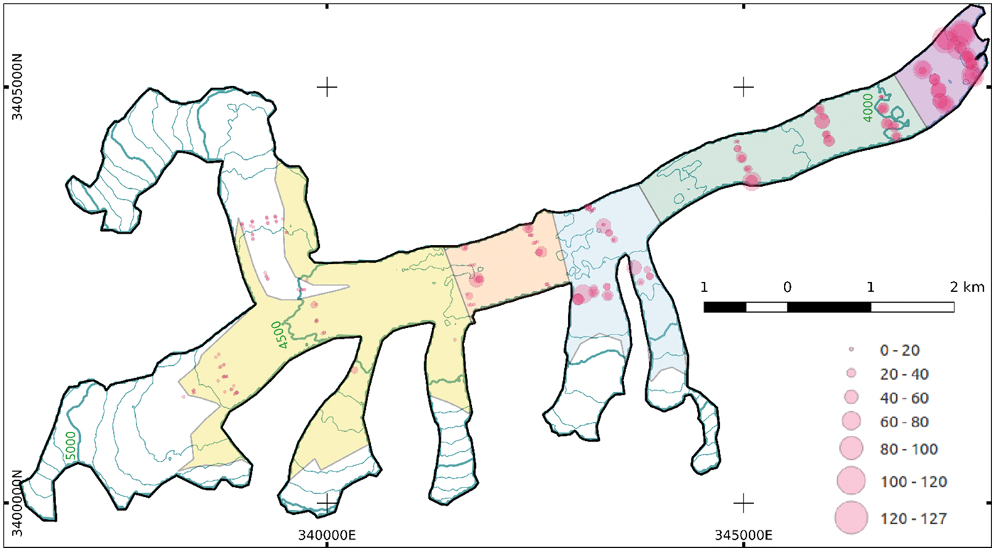
Fig. 1. A map of Satopanth Glacier (30.73N, 79.32E; the Central Himalaya) showing the glacier boundary (thick black line), debris extent (coloured shaded polygons) and the location of ablation stakes (filled circles). The size of the circles denotes the corresponding debris thickness value (in cm). The debris-covered area is partitioned into five different subzones as shown with shaded polygons of different colours (see text for details). The 100 m surface-elevation contours are plotted with thin blue lines, with thicker lines being used every 500 m. The thicker contour lines on the main trunk are labelled with the corresponding elevation values in meters.
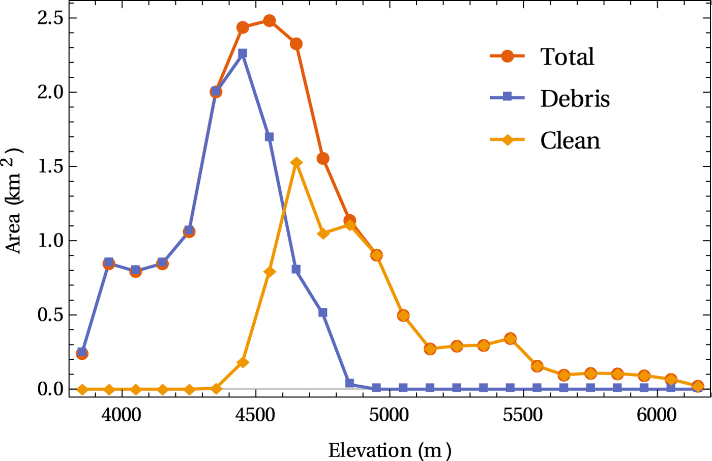
Fig. 2. Area-elevation distribution of the clean-ice area, debris-covered area and total glacierised area for Satopanth Glacier. The binsize is 100 m.
Existing records suggest that Satopanth Glacier is in a retreating phase since at least 1936, with an average frontal retreat rate of ~6 m a−1(Nainwal and others, Reference Nainwal, Banerjee, Shankar, Semwal and Sharma2016). It has a relatively stagnant lower ablation zone where the ice flow speed is less than 5 m a−1. The lower ablation zone has been thinning at the rate of ~0.4 m per year over the past half century or so (Nainwal and others, Reference Nainwal, Banerjee, Shankar, Semwal and Sharma2016).
All of the above characteristics are quite typical of debris-covered glaciers in the Himalaya (Scherler and others, Reference Scherler, Bookhagen and Strecker2011b), and Satopanth Glacier can be considered a representative debris-covered Himalayan glacier.
Field data
Glaciological mass-balance measurements on Satopanth Glacier were initiated in the ablation season of 2014 with a small number of bamboo stakes, and are continuing until now with the network being extended to up to ~60 stakes (Fig. 1). Most of the stakes are arranged into ten transverse lines at the main trunk below 4600 m elevation, and a few lines across some of the tributaries. Each of these lines consists of about five stakes. Most of the stakes are in the debris-covered parts, with measured debris thickness at stake locations varying between 0.02 and 1.27 m.
To install the stakes, we dug pits in the supraglacial debris exposing the glacial ice, drilled holes into the ice using a Heucke steam drill, and inserted the bamboo stakes. Each stake was ~2 m in length and depending on location up to three stakes, joined by binding wires, were inserted into the drill hole. After installation, the pits were back-filled with debris. Subsequently, the height of the stakes above the debris surface was monitored biweekly (Fig. S1), with an accuracy of ~2 cm. Due to the size of the glacier, each set of measurements took ~2–3 days to complete depending on weather conditions. The stake positions were monitored using a pair of Trimble R6 Global Navigation Satellite System receivers.
One specific problem encountered due to the local variability of debris thickness was that once a stake was about to melt out, it was not possible to install a stake at a nearby location with the same debris thickness and maintain continuity of the ablation data from that location. The nearby locations would invariably have different debris thickness values, and thus, different ablation rates. Also, the debris interfered with the stability of the stakes in various ways. For example, the bottom of the debris layer was typically saturated with meltwater and would cause some of the stakes to rot and break. This problem could be mitigated to some extent by using painted stakes. Sometimes a stake would not fall over even when it had fully melted out of the ice, remaining planted in the thick debris instead. However, such cases could be identified because these stakes, once melted out of the ice, yielded too low an ablation rate. Overall, due to issues like lost or broken stakes, delay in re-installing fallen stakes, bad weather conditions, equipment malfunctions, etc., several data gaps exist in our records.
In each ablation season, we began our periodic measurements during the last week of May and continued them until the end of October. To measure the ablation of sub-debris ice, we kept to the snow-free stakes in the lower part of the glacier in the early ablation period, and progressively moved up as upper stakes became snow free. Depending on year, by mid June to beginning of July, all the stakes became accessible.
The pits dug for installation of stakes and re-installation of fallen stakes were utilised to measure the debris thickness distribution. Until now, we have measured debris thickness at 191 locations. However, these pits are not uniformly distributed across the glacier ablation zone. They are mostly in the neighbourhood of the planted stakes, along the transverse transects mentioned above (see Fig. 1).
Data analysis
Characterisation of the spatial variability of debris thickness
To estimate debris-thickness distribution, we binned the thickness data from the pits. The bin sizes varied from 5 cm for thin debris to 10, 15 and 25 cm as debris thickens (Fig. S2). This does not compromise the accuracy of mass-balance estimates as the variation of ablation rate with debris thickness is weaker for thicker debris (Eqn 1). To analyse the variability of debris distribution at smaller spatial scales, we partitioned the entire debris-covered ablation zone into five subzones, such that for each of these subzones we have at least 30 point measurements of debris thickness available (Fig. 1), which were used to compute the frequency distribution of debris thickness at each of the subzones (Fig. S2). We acknowledge that the choice of the zone boundaries is somewhat arbitrary and that adds to the uncertainty in the mass-balance computation. Accordingly, we considered a large (30%) uncertainty in the area of the subzones while estimating the errors in our computation of sub-debris ablation as described later.
Outliers in the ablation rate data
We removed a few outliers in the stake data before further analysis. Some of the outliers were related to broken or melted-out stakes. Due to the thick debris layer, a few of these stakes remained standing after melting out and showed spuriously low or zero ablation rates. Some of the outliers were likely also due to mistakes while taking manual readings. We tried to maintain photographic records of each measurement with scale (Fig. S1), and a few mistakes could be corrected using such photographs. However, in some cases the quality of the field photographs were not good enough or photographs could not be taken, and we preferred to discard the individual observations in case it showed unusually large deviations compared to neighbouring stakes. Finally, we have 262, 383 and 334 ablation measurements available from the debris-covered ablation zone of Satopanth Glacier during the ablation season of 2015, 2016 and 2017, respectively. The number of ablation rate measurements from the debris-free part of the glacier is 24, 70 and 45, respectively.
Relative performance of elevation and debris-thickness-dependent parameterisations of ablation rate
The previous discussions on the influence of the variability of elevation (z) and debris thickness (d) on sub-debris ablation rate indicate that the best method to obtain an accurate estimate of the local sub-debris ablation rate anywhere on the debris-covered ablation zone would be to parameterise ablation as a function of both elevation and debris thickness. In practice, however, the utility of such a method is limited as, for example, one needs the joint probability distribution of both elevation and debris thickness to obtain glacier-wide mean ablation. While elevation distribution may easily be obtained with remote-sensing methods, it is difficult to obtain the debris-thickness distribution within each of the elevation bands. With field methods, it is practically impossible to get the distribution for each elevation band as that would require digging a very large number of pits. The remote-sensing methods to determine debris thickness either do not work well in the thick debris ($\gtrsim 50$ cm) limit, or have significantly large uncertainty in this limit (Rounce and others, Reference Rounce, King, McCarthy, Shean and Salerno2018). A way out of this problem is possible in case either the variability of elevation or that of debris thickness has a dominant control over the local ablation rate variability. If that is the case, the point-scale ablation data can be parameterised as a function of a single variable only, and the knowledge of the distribution of that specific variable is sufficient to compute glacier-wide ablation.
To check whether it is the local elevation or the debris thickness that has a stronger control on the observed ablation rate variation, we fitted all the ablation data for any given observation period separately to an elevation-dependent and a debris-thickness-dependent function. Following the standard glaciological protocol, the elevation-dependent form (b z(z)) was taken to be a quadratic polynomial in elevation (Kaser and others, Reference Kaser, Fountain and Jansson2003). The debris-dependent fit function (b d(d)) was assumed to be of the form given in Eqn (1) (Anderson and Anderson, Reference Anderson and Anderson2016). To quantify the goodness of fits, we computed the root-mean-squared deviation (RMSD) of the observed versus fitted ablation rates for each of the fits. The adjusted R 2 for each of the fits were also computed. The RMSD over all the fits and adjusted R 2 averaged over all the fits obtained from the two methods were compared for each of the years. We also analysed the correlation coefficients among debris thickness, elevation and ablation rate.
Computation of mean specific ablation over the debris-covered area with an elevation-dependent interpolation (method-I)
We denote the standard glaciological mass-balance estimation protocol (Kaser and others, Reference Kaser, Fountain and Jansson2003) as method-I. Here, for each of the measurement periods (t i − Δt i, t i), we collated all the available stake data from the debris-covered portion of the ablation zone, and fitted them to a smooth (three-parameter) quadratic function of elevation b z(z, t i) (e.g., Fig. 3a). The mean specific ablation rate was obtained by averaging over the hypsometry of the debris-covered part of the ablation zone and over all the measurement periods as follows,

where, A j is the map area within the elevation band (z j, z j + Δz).

Fig. 3. Figures (a) and (b) show examples of smoothing functions b I(z) and b II(d) fitted to the same ablation data set (Year 2016, Julian day 187±1). In sub-figure (a) symbol colours denote debris thickness, and in sub-figure (b) symbol colours represent elevation. See text for detailed discussion.
To estimate the uncertainty in b I due to the corresponding uncertainties in the measurement of ablation at the stakes and that in the area-elevation distribution, we employed a Monte Carlo method. We repeated the steps outlined above 1000 times, but each time adding an independent zero-mean Gaussian noise to the individual observations of ablation, and the area fraction at each bin. The Gaussian noise in ablation data was assumed to have a standard deviation equal to twice the estimated measurement uncertainty of each stake-height observation (estimated to be ~4 cm). Similarly, a nominal 20% uncertainty in area-elevation distribution was incorporated with the latter random noise. This uncertainty is partly due to the uncertainty in mapping the glacier boundary (particularly in the debris-covered parts), and due to the uncertainty in the 10 m resolution Cartosat-1 digital elevation model (https://bhuvan.nrsc.gov.in) used here. Another source of uncertainty in the estimated total ablation was related to the best-fit smooth quadratic function b z. For each elevation bin, the RMSDs of the observed values from the fitted curve were computed over all the measurement periods. This mean RMSD was assumed to be equal to the corresponding prediction error for the elevation bin. Again, a zero-mean random Gaussian noise with standard deviation equalling the mean RMSD was added to the interpolated values in the Monte Carlo. Twice the standard deviation of the set of 1000 b I-values obtained in the Monte Carlo procedure was taken to be the 2σ uncertainty estimates.
The algorithm steps of the method are as follows:
1. We divide the observed region into N e elevation bands. The bands are 100 m wide and the area of each band, A j is shown in Fig. 2.
2. The observation times are denoted by $t_i, \,i=1,\,\ldots ,\,N_t$
 and the time periods between them by Δt i ≡ t i − t i−1. The observation times are given in Supplementary Figures S3–S5.
3. Equation (2) gives the expression for the average ablation rate estimated using method I. It can be written as,
(3)$$ b_{\rm I} = {\displaystyle {1} \over {A}}\sum \limits_{\,j=1}^{N_e}A^z_j \bar b_z(z_j), $$(4)$$ {\bar b}_z(z_j) = {\displaystyle{1} \over {T}}\sum \limits_{i=1}^{N_t} b_z(z_j,t_i)\Delta t_i, $$where A is the total area of the observation region, $A = \sum \nolimits_{j=1}^{N_e} A_j$ and T is the total observation time period, $T = \sum \nolimits_i\Delta t_i$.

The uncertainty in b I is computed using the the following algorithm:
For n = 1 to 1000,
1. Compute the parameters, a ni, b ni, c ni by fitting the data, b obs(z m, t i) + Δb obs(z m, t i) to the quadratic function b zn(z, t i) = a ni + b niz + c niz 2. Where b obs(z m, t i) is the observed ablation at the m th stake at elevation z m, during the i th time period and Δb obs(z m, t i) is a Gaussian noise with standard deviation 4 cm.
2. Compute the RMSD at each time period,
(5)$$ \Delta b_{zn}(t_i)=\sqrt{{\displaystyle{1} \over {N_e}}\sum_m\left(b_{zn}(z_m,t_i)-b^{obs}(z_m,t_i)\right)^2}. $$3. Compute the average RMSD over all the time periods,
(6)$$ \Delta \bar b_{zn}=\sqrt{{\displaystyle{1} \over {N_e}} \sum_i\left(\Delta b_{zn}(t_i)\right)^2}. $$4. Compute the net average ablation rate, b In,
(7)$$ b_{{\rm I}n}={\displaystyle{{\left(\sum \nolimits_j A_j+\Delta A_{\,jn}\right)} \left({\bar b}_n(z_j)+\Delta{\bar b}_n(z_j)\right)} \over {\sum \nolimits_j\left(A_j+\Delta A_{\,jn}\right)}}, $$where A j is the estimated area of the j th elevation zone, ΔA jn is a Gaussian noise with standard deviation equal to 0.2A j and $\Delta \bar b_n(z_j)$ is a Gaussian noise with standard deviation equal to $\Delta \bar b_{zn}$.5. The mean value and twice the standard deviation of this distribution of 1000 values of b I are the reported values of the most probable value of b I and its uncertainty.


Computation of mean specific ablation over the debris-covered area with a debris-thickness-dependent interpolation (method-II)
For the debris-covered part of the ablation zone, we used an alternative method where point-scale ablation-rate data were interpolated as a smooth function of debris thickness only. We denote this method as method-II. In method-II, all the observed ablation rates in a given observation period were fitted to a smooth debris-thickness-dependent function b d(d) (e.g., Fig. 3b). We chose b d(d) to be of the form given in Eqn (1) (Anderson and Anderson, Reference Anderson and Anderson2016). The parameters b 0 and d 0 were obtained separately for each observation period (denoted by i). Then, to obtain the mean sub-debris melt, the fitted b d for each of the periods were averaged over the area distribution of debris thickness. To obtain the area distribution, we used the five subzones (Fig. 1) and the measured frequency distribution of the debris thickness in each of these zones (Fig. S2). The mean specific ablation rate over the debris-covered ablation zone was then computed as,

where, $A^n_j$ are the areas with debris thickness values in the range (d j, d j + Δd j) for the n-th subzone (see Fig. 1 for definition of the subzones).
The uncertainty in the estimates of the mean specific ablation (b II) due to measurement and mapping errors, and prediction errors in the fitted forms were computed with 1000 Monte Carlo iterations with the addition of appropriate Gaussian noise just as for method-I. The width of the noise in the ablation rate was again assumed to be 4 cm. The prediction errors due to fitting were simulated in a similar manner using the RMSD for each debris-thickness bin over all measurement periods. Since, demarcation of the subzones is somewhat arbitrary, a larger 30% noise was added to the coefficients ($A^n_j$ ). Within each subzone, the debris distribution was also recomputed in each Monte Carlo step by adding a zero-mean Gaussian noise with a standard deviation of 4 cm to the debris-thickness value. Finally, the standard deviation of the 1000 independent estimates as obtained in the Monte Carlo procedure was used to estimate the 2σ uncertainty in b II.
The algorithm steps of the method are as follows:
1. We divide the observation region into five zones, shown in Fig. 2. The debris thickness distributions in these five zones are plotted in Figure S2.
2. We divide the debris thickness into N d bands, denoted by $d_j,\,j=1,\,\ldots ,\,N_d$
. We define Δd j ≡ d j+1 − d j.3. We estimate the area in the l th zone which has a debris thickness in the j th band, $A^l_j$
, to be the fraction of the debris thickness observations in the l th zone that were in the j th band multiplied by the area of the l th zone.

Equation (7) gives the expression for the average ablation rate estimated using method II. It can be written as,


The uncertainty in b II is computed using the the following algorithm:
For n = 1 to 1000,
1. Compute the parameters, b 0in, d 0in by fitting the data, b obs(d m, t i) + Δb obs(d m, t i) to the function, b d(d), given in Eqn. (1). Where b obs(d m, t i) is the observed ablation at the m th stake with debris thickness d m during the i th time period and Δb obs(d m, t i) is a Gaussian noise with standard deviation 4 cm.
2. Compute the RMSD at each time period,
(12)$$ \Delta b_{dn}(t_i)=\sqrt{{\displaystyle{1} \over {N_d}}\sum_m\left(b_{dn}(d_m,t_i)-b^{{\rm obs}}(d_m,t_i)\right)^2}. $$3. Compute the average RMSD over all the time periods,
(13)$$ \Delta {\bar b}_{dn}=\sqrt{{\displaystyle{1} \over {N_t}}\sum_i\left(\Delta b_{dn}(t_i)\right)^2}. $$4. Compute the net average ablation rate, b IIn,
(14)$$ b_{{\rm II}n}={{\displaystyle{\left(\sum \nolimits_{\,j=1}^{N_d}\sum \nolimits_{l=1}^5 \left(A^l_j+\Delta A^l_{\,jn}\right)\right) \left(\bar b_{dn}(d_j)+\Delta\bar b_{dn}(d_j)\right)}} \over {\sum \nolimits_{\,j=1}^{N_d}\sum \nolimits_{l=1}^5\left(A^l_j+\Delta A^l_{\,jn}\right)}}, $$where $A^l_j$ is the estimated area of the j th debris thickness band in the l th zone, $\Delta A^l_{jn}$ is a Gaussian noise with standard deviation equal to $0.3A^l_j$ and $\Delta \bar b_{dn}(d_j)$ is a Gaussian noise with standard deviation equal to $\Delta \bar b_{dn}$.5. The mean value and twice the standard deviation of this distribution of 1000 values of b II are the reported values of the most probable value of b II and its uncertainty.


Biases due to the number of stakes used
We investigated the robustness of estimated b I and b II with respect to the number of stakes used by a Monte Carlo method with repeated computation of the two quantities with randomly chosen subsets of all the available stakes. First, we computed the net ablation rate over the debris-covered parts of the ablation zone with all the available stakes (N) using both the methods (I and II) following the procedure described above. Then, the net ablation computation for both the methods was repeated 300 times each, for randomly chosen subsets of 3N/4, N/2 and N/4 stakes. In case the randomly chosen subset of stakes did not have a single observation in any of the measurement intervals, that subset was ignored. The distribution of the estimates for b I and b II for each of the sample sizes was then analysed to investigate the possible uncertainties and biases in the result obtained as a function of the number of stakes used for both the methods.
Results and discussions
The spatial variability of debris thickness
The measured debris thickness values at the pits ranged from a couple of cm to more than 100 cm, with a highest observed debris thickness of 127 cm. In general, the debris layer thickened down-glacier (Fig. 4). The mean debris thickness of the five subzones defined in Figure 1 increased with decreasing mean elevation, varying from 7 to 61 cm. This trend of a general down-glacier increase in debris thickness is also evident from the fact that the debris thickness and elevation at all the 191 pits were anti-correlated with a correlation coefficient of −0.64 (p < 0.0001).

Fig. 4. The variation of debris thickness on Satopanth Glacier is shown with open symbols representing debris thickness measured at individual pits. Different symbol colours represent different subzones marked in Figure 1. The mean and standard deviation of the debris thickness in each of the zones are shown using solid circles with bars.
The above increase of the local mean of debris thickness down-glacier is accompanied by a comparable increase in the local variability of debris thickness. The standard deviation of debris thickness within each of the subzones increased along with the corresponding mean, such that it was at least half the mean or more (Fig. 4). To give an example, in the lowermost subzone the observed debris thickness varied between 2 and 127 cm, with a mean of 61 cm and a standard deviation of 30 cm. The observed debris-thickness distribution for all the subzones is given in the Supplementary Figure S2.
This trend of nearly monotonic down-glacier increase of both the mean debris thickness and its local spatial variability is consistent with the data from other debris-covered glaciers in the Himalaya and elsewhere (Mihalcea and others, Reference Mihalcea2006; Zhang and others, Reference Zhang, Fujita, Liu, Liu and Nuimura2011; Nicholson and Mertes, Reference Nicholson and Mertes2017; Banerjee and Wani, Reference Banerjee and Wani2018; Nicholson and others, Reference Nicholson, McCarthy, Pritchard and Willis2018). The increasing trend of the local mean debris thickness has been explained in terms of the emergence of englacial debris, and the decline of glacier ice-flow velocity towards the terminus (Kirkbride and Deline, Reference Kirkbride and Deline2013; Anderson and Anderson, Reference Anderson and Anderson2016, Reference Anderson and Anderson2018). However, a theoretical understanding or model reproduction of the fluctuating part of the debris-thickness distribution discussed above is not available at present. A critical role of gravity-driven non-diffusive debris redistribution processes, induced by the dynamic thermokarst topography that characterises the debris-covered ablation zone, is expected in creating and maintaining the observed inhomogeneous debris distribution (Moore, Reference Moore2018; Nicholson and others, Reference Nicholson, McCarthy, Pritchard and Willis2018).
A comparison of the controls of elevation and debris thickness on the sub-debris ablation rate
Our analysis shows that the debris-thickness-dependent smooth function b b(d) provides a better description of the mass-balance variation than the elevation-dependent function b z(z) for all the observation periods (Fig. 3 and Supplementary Figs S3–S8), in the sense that the former obtains a systematically higher R 2 for the fits (Table 1). The ablation rates for any given period have a larger scatter around the elevation-dependent fitted forms than the debris-thickness-dependent forms. All the fitted profiles for the3 years given in Supplementary Figures S3–S8 conform to this general trend. With debris-thickness-dependent fits, the mean RMSD over all the fits in a year varies between 0.41 and 0.52 cm d−1 among the 3 years. In comparison, the corresponding RMSDs with elevation-dependent fits are ~50% higher, with mean values ranging between 0.60 and 0.77 cm d−1 for the years 2015, 2016 and 2017. These trends indicate that the variation of ablation rate over the debris-covered parts of Satopanth Glacier is better described by the debris-dependent form b d than the elevation-dependent form b z.
Table 1. A summary of ablation data from the debris-covered part, and the estimates of mean annual sub-debris ablation rates using method-I that uses elevation-dependent interpolation (b I) and method-II that uses debris-thickness-dependent interpolation (b II)

Note that total observation period for each of the years is given in Julian day, root-mean-square deviation (RMSD) is computed over of all the fits in a given year, and adjusted R 2 is averaged over all the fits in a given year. See text for further details.
In addition, the correlation between variation of debris thickness and that of ablation rate (−0.53 to −0.57; p < 0.0001) is systematically stronger than that between variations of elevation and ablation rate (0.32–0.44, p < 0.0001) for all the 3 years. This strengthens the above claim that local debris thickness is a better predictor of local ablation rate.
The improved accuracy obtained with the debris-thickness-dependent fitting functions in smoothing/interpolating the sub-debris ablation data makes a strong case for using method-II, which interpolates ablation rate as a function of debris thickness alone for each of the observation periods to compute mean sub-debris ablation. In fact, in this method, the weaker elevation dependence of ablation rate is implicitly taken in to account to some extent due to the anti-correlated variation of elevation and debris-thickness observed (a correlation coefficient of −0.64, p < 0.0001).
Since the overall properties of the debris-thickness distribution of Satopanth Glacier is similar to that of other debris-covered Himalayan glaciers as discussed in the previous subsection, it may be expected that the debris-thickness-dependent interpolation would, in general, be a more accurate method for debris-covered ablation zones of other glaciers as well. As mentioned before, an interpolation method that uses the joint distribution of elevation and debris may be more accurate. However, from a practical point of view, it would be difficult to obtain an accurate debris-thickness distribution for each of the elevation bands through field measurements due to logistical issues. Remote-sensing methods can be useful, but they are not very accurate in the thick-debris limit (Rounce and others, Reference Rounce, King, McCarthy, Shean and Salerno2018). In this context, method-II presented here may be a good compromise.
Mean sub-debris ablation using method-I and method-II
Method-I, where ablation rates are interpolated as a function of elevation (Eqn 2), yielded mean sub-debris ablation rates of 1.25 ± 0.14, 1.35 ± 0.16 and 1.56 ± 0.17 cm d−1 for the ablation season of 2015, 2016 and 2017, respectively. With method-II, which is based on a debris-thickness-dependent interpolation (Eqn 7), the corresponding estimated mean sub-debris ablation were 1.52 ± 0.19, 1.71 ± 0.30 and 1.50 ± 0.21 cm d−1, respectively. The distribution of the values generated in the Monte Carlo for the two methods are shown in Figure 5.
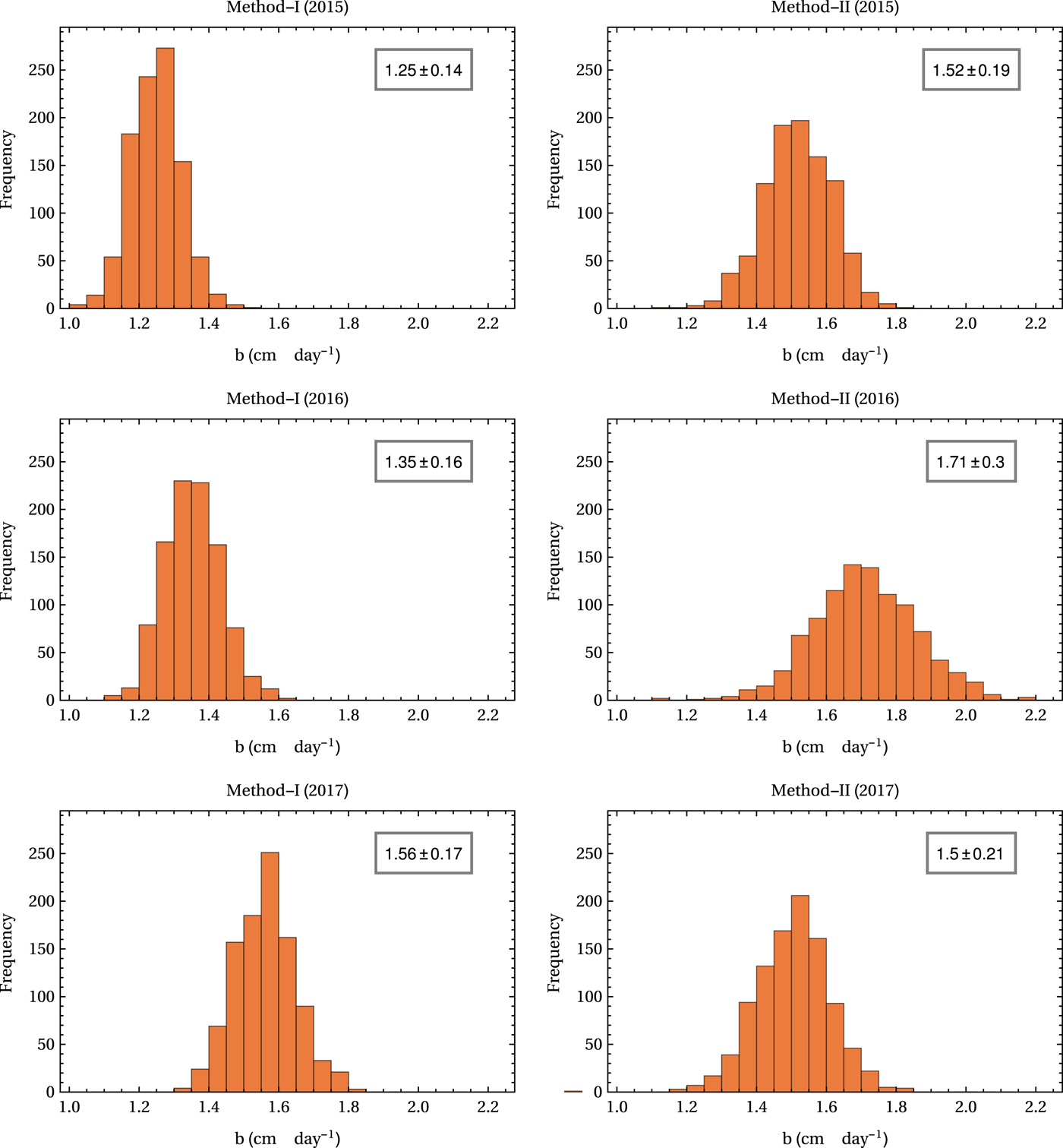
Fig. 5. The distribution of mean specific ablation rates over the debris-covered ablation zone generated in the Monte Carlo simulations for method-I and method-II. The mean and 2σ error bars are given in the insets.
Despite the tighter fits obtained with the debris-dependent interpolation scheme used in method-II, the differences between the estimates obtained in the two methods are not significant when the uncertainties in the corresponding values are considered (Table 1). For the ablation seasons of 2015 and 2016, the estimated values of b I are ~20–25% smaller than the corresponding estimates of b II, while for 2017, b I is a few per cent higher than b II. However, none of these differences are significant given the uncertainties present in the estimates. The interannual variability of mean sub-debris ablation is also not significant given the uncertainties.
The above results imply that the empirical elevation-dependent quadratic smooth interpolating function does well in predicting the mean ablation in any elevation band, even though it does not capture the variability of ablation rate within that elevation band. This could be because of the relatively large number of stakes used in this study, so that within each elevation band a few stakes with different debris thicknesses are available (Fig. 3a, Supplementary Figs S3–S5). The arrangement of stakes along transverse lines (Fig. 1) also helps in sampling the debris distribution within an elevation band. If these arguments are correct, then discernible differences between estimates from the two methods may be present when data from only a few stakes are available. This is discussed in the next subsection.
We also note that despite the better fits to ablation data obtained in method-II, the relative uncertainties were somewhat higher in this method (13–18%) as compared to that in method-I (11–13%). This was likely related to possible large uncertainties in partitioning the debris-covered area into the subzones and the limited number of debris-thickness measurements (~30) that were available for each of the subzones. The uncertainties of the method-II estimates could be brought down further with more detailed measurements of the debris-thickness distribution in the ablation zone.
Accuracy of the estimates of mean sub-debris ablation as a function of the number of stakes used
The total number of stakes where some ablation data were available (N) varied from 55 to 83 in the 3 years (Table 1). We note that this included reinstalled stakes, and the actual number of stakes available for any given observation period was less with a mean number of stakes of ~30 (Table 1). In the numerical experiments, where only a fraction of available stakes were used for the ablation rate calculations, the estimated ablation for any given random subset of the data had biases for both the methods. Both positive and negative biases were observed depending on the chosen random subset, and the biases were systematically larger as the number of stakes used went down from N to N/4. For method-I and using 3N/4 stakes, the estimates were within the uncertainty band of ablation estimated with the full data set (Fig. 6) for 2015 and 2017. Only in 2016 did some of the random subsets underestimate the mean ablation significantly. The observed deviations in this method were significant for N/2 stakes. For method-II, the spread in the estimates from random subsets of the stakes was in general smaller compared to that in method-I (Fig. 6). Here, even the subsets with N/2 stakes produced estimates that were within the uncertainty band (except in 2016). Only with N/4 stakes significant underestimation of mean ablation was observed for method-II. Generally larger uncertainties in 2016 may be related to the two observation periods where data from only ~10 stakes are available (Supplementary Figs S4 and S7).
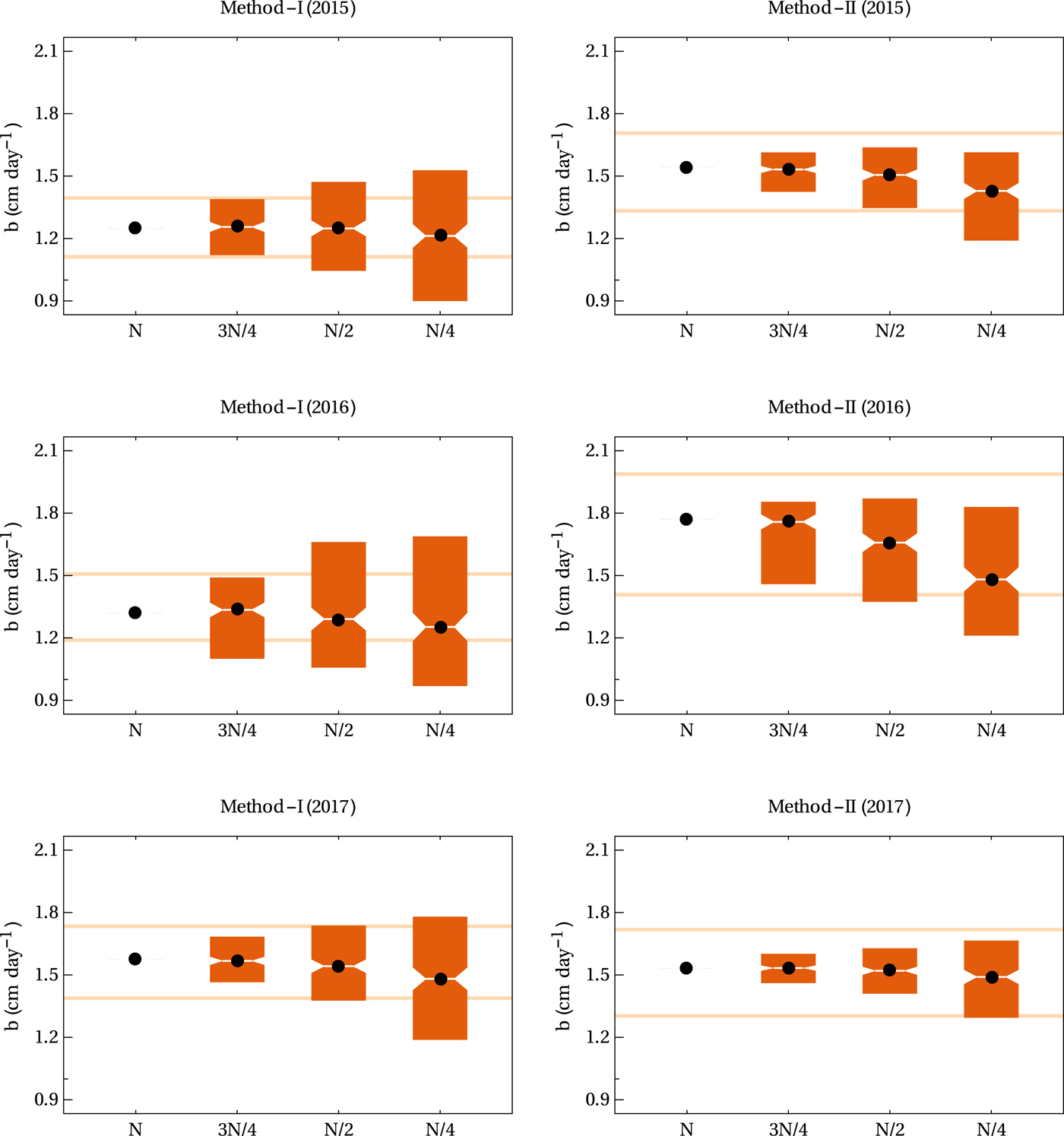
Fig. 6. The distribution of the estimated mean sub-debris specific ablation (b) over the ablation zone of Satopanth Glacier as computed using method-I and method-II for the 3 years with randomly selected subsets of the data. The horizontal axis denotes the number of stakes used in the calculations. Either all the N stakes, or 300 random subsets with 3N/4, N/2 and N/4 stakes each were used to compute the mean sub-debris ablation rate. Values of N were 55, 73 and 83 for 2015, 2016 and 2017, respectively. The vertical bars depict the spread of the distribution from 5 to 95 percentile. The black dots represent the median value. Horizontal orange lines show the 2σ confidence band for the estimated ablation rate (see Table 1) for reference.
As discussed in the previous subsection, debris-dependent fits work better than the corresponding elevation-dependent forms. However, that did not translate to any differences between the net balance estimates from the two methods beyond the limits of the corresponding uncertainties. In this context, the set of estimates using smaller subsets of the whole data as described above established a clear advantage of method-II over method-I. The method-II estimates were seen to be more robust when a reduction in the number of stakes was applied. This was likely a consequence of the tighter fits obtained with the debris-dependent parameterisation. In contrast, the elevation-dependent smoothing procedure was able to capture the mean ablation in any given elevation band accurately only when a relatively large number of data points were available. With a small number of stakes the fluctuation caused by the variability of debris thickness did not get averaged out, possibly resulting in large biases in the mean ablation estimated using method-I as compared to that from method-II.
Fountain and Vecchia (Reference Fountain and Vecchia1999) demonstrated that on a small (<10 km2) clean alpine glacier, 5–10 stakes are enough to obtain an accurate mass-balance estimate, when an elevation-dependent regression method is used. On Satopanth Glacier, when all the available N stakes were used, the mean number of available records for the observation period was ~30 (Table 1). Above analysis shows that while using method-II, accurate subdebris ablation could be obtained for Satopanth Glacier even with N/2 stakes. This may indicate that ~15 stakes may be sufficient to obtain accurate mass-balance estimates for the debris-covered ablation zone (~10 km2) of Satopanth glacier provided, (1) continuous measurements are carried out without any data gaps, (2) the stakes cover a range of debris thickness values, (3) a detailed measurement of the debris-thickness distribution is performed, and (4) a debris-thickness-dependent interpolation is used. Note that with a smaller sized debris-covered glacier, the total number of stakes cannot be reduced proportionately as sampling the range of debris-thickness values would become an issue. Also, an observation period with a large number of missing stakes can be detrimental to the accuracy of the estimate. Similar analysis with data from other debris-covered glaciers may be necessary to determine the optimal number of stakes to be used on this type of glacier.
Conclusions
We measured surface ablation on debris-covered Satopanth Glacier (Central Himalaya) using a network of up to 56 stakes during the ablation seasons of 2015, 2016 and 2017. The debris-thickness distribution was obtained by direct field measurements at 191 pits. Using the extensive ablation data, we established that a debris-thickness-dependent smoothing curve performed better than an elevation-dependent regression, in describing the spatial variability of surface ablation at any given observation period. We utilised the debris-dependent smooth fits to the ablation data, averaged over the debris-thickness distribution over the glacier surface, to obtain mean sub-debris ablation rates on Satopanth Glacier of 1.52 ± 0.19, 1.71 ± 0.30 and 1.50 ± 0.20 cm d−1 during 2015, 2016 and 2017, respectively. In comparison, the standard glaciological method obtained ablation rates of 1.25 ± 0.14, 1.35 ± 0.16 and 1.56 ± 0.17 cm d−1 for the 3 years. While the above differences in estimates from the two methods are consistent with each other given the corresponding uncertainties, biases are not negligible if the number of stakes with data were low. It was seen that ~15–30 stakes are needed for an accurate mass-balance estimate on Satopanth Glacier. However, the debris thickness at the stakes must span a wide range. The accuracy of the estimates using a debris-dependent method may be improved further with more detailed measurement of the debris-thickness distribution.
The glaciological ablation data presented in the paper is accessible at https://osf.io/kr2q7/
Acknowledgments
We acknowledge the help from Gajendra Badwal, Surendra Badwal, Nepalese porters, Sourav Laha, Reshma Kumari, Aditya Mishra, Prabhat Semwal, Tushar Sharma and people from Mana village during the field work. The field measurements on Satopanth glacier were supported by The Institute of Mathematical Sciences, Chennai. We thank the anonymous reviewers, the editors Nicolas Cullen and Hester Jiskoot for useful comments and suggestions.
Supplementary Materials
The supplementary material for this article can be found at https://doi.org/10.1017/jog.2019.48.


 Open access