


Introduction
With water supplies and the hydroelectric power obtained from them in great demand, the water equivalent of snow packs represents an important resource on a world-wide basis. The effective management of water resources requires adequate knowledge of the snow-pack extent, depth, density, and wetness. At present, trained individuals traverse snow courses to obtain snow depth and weight using Mt Rose tubes at selected sites. Some additional information is obtained by the use of “pressure pillows” to weigh the snow at automatic stations; other systems involve the attenuation of gamma rays by absorption in snow layers.
The field methods in current use are of great value in providing information to permit forecasting of water run-off; “point” measurements are combined by statistical methods to yield a representative value for a basin. However, automatic stations and airborne systems for repetitive assessment of snow-pack depth, density, and wetness would have important applications in water-resource management and flood prediction, particularly at times of rapid change. Other applications involving airborne or satellite-based techniques include measurement of ice thickness on shipping lanes and in the polar regions, and snow cover on remote areas.
Remote-sensing systems are being developed by the scientific community, based on both passive and active electromagnetic (EM) techniques. Considerable literature is already available. Some of the references that are particularly relevant to this paper are Saxton (1950), Cumming (1952), Jiracek (1967), Evans and Smith (1969), and Waite and MacDonald (1969). A “swept-frequency” EM system for snow-pack measurements was described by Linlor (1973), for which the models analyzed in the present paper represent the theoretical basis. In a simple form, that system would consist of an antenna that transmits a set of sequential fixed frequencies (thus approximating a “swept-frequency” operation). A selected frequency would be transmitted within a pulse having sufficient duration to include between 10 and 100 cycles, thus nearly equivalent to “continuous-wave” (CW) operation. With the antenna on an aircraft having an altitude of 150 m or higher, the pulse having a duration of 1 μs or less would be completed before the specular reflection from the snow pack could reach the antenna. Hence, the same antenna could be used for transmission and reception. Amplitude and phase of the reflected signals would be recorded for the desired frequency range.
The present work is part of a broad program having many interdependent aspects. The ultimate goal is a remote-sensing system that can be flown in an aircraft or satellite to obtain repetitive, synoptic measurements of snow-pack areal extent, depth, density, and wetness. Combinations of passive and active EM instrumentation are envisaged, the latter including short-pulse as well as the pulsed swept-frequency measurements described above. For flight experiments, ground truth is needed, and suitable instrumentation to obtain such information is being developed. Snow wetness, which is one of the most important parameters determining the EM response, may be measured at the surface by electrical techniques described by Linlor and Smith (1974) and by Linlor and others (1974).
Our proposed active EM airborne remote-sensing system is a direct spin-off from some of the basic research in the NASA space exploration program. Prior to the Apollo 17 mission, theoretical analyses and computer codes were used to obtain the response of (hypothetical) plane layers on the moon, assuming incident plane EM waves, as described by Ward and others (1968) and by Linlor and others (1970).
During the manned lunar exploration program, consideration was given to application of the EM techniques to various layered models of snow, ice, water, and earth, and certain problems inherent in such applications were recognized. The electrical parameters of snow, in situ, are known to cover a wide range of values depending on the density, temperature, free-water content, and other variables such as sequences of rain, freezing, and thawing. There also are important practical considerations, such as the effects of earth roughness, snow surface roughness, reflection from inadvertent radiators (telephone or power lines in the vicinity of the reflection zone), and similar complications. A few remarks are made later in this paper concerning the limitations arising from practical applications.
As an initial step, this paper is a theoretical study only, and does not include consideration of the size, weight, cost, or performance characteristics of a working system. The basic objective is to present the results of calculations for a variety of models, directed toward such questions as:
-
1 For sets of earth conditions, how does the reflection coefficient depend on the dielectric constant, loss tangent, and thickness of the snow layers?
-
2 For various sets of snow layers, how does the reflection coefficient depend on the dielectric constant and loss tangent of the earth ?
-
3 For an invariant amount of water-equivalent in the totality of the layers, how does the reflection coefficient change when the individual layers of snow (or ice) are interchanged in various sequences?
Outline of Theory
The principle of the electromagnetic interactions on which the proposed system is based can be explained by the model shown in Figure 1. The model represents the simple case of a thin sheet separating two semi-infinite media. Stratton (1941) derives the following expression for the power reflection coefficient R at normal incidence assuming that the three media have zero conductivity and vacuum permeability:

Fig. 1. Three-layered model.
where the amplitude reflection coefficients at the interfaces are r 12 and r 23, d is the sheet thickness, and α2 = 2π/λ2 where λ2 is the wavelength within the sheet. The power reflection coefficient R is what an airborne instrument would measure and is given by
where r represents the amplitude reflection coefficient for the model. Unless explicitly stated otherwise, we use amplitude reflection coefficients in this paper.
The sequential minima for r occur at the frequencies
where f is the frequency in Hz and d is the thickness in meters. The permittivities of the three dielectrics are ε 1 ε 2 and ε 3 in F/m, and the relative permittivities are K 1 , K 2 and K 3 , dimensionless.
For the assumed lossless media, the maxima for r are equal to r 13, namely, the reflection coefficient with layer 2 effectively absent; these occur at the sequental frequencies
Letting K 1 = 1.0 for air, from Equations (4) and (7) we obtain

Fig. 2. Reflection amplitude versus thickness.
A solid ice layer over water is an example of a three-layer system. Let us make the simplifying assumptions that the ice and water are lossless, and have dielectric constants of 3.2 and 81 respectively, independent of frequency. A plot of Equation (1) is shown in Figure 2, with thickness d of medium 2 plotted in units of λ2, versus amplitude reflection coefficient of the model. For ice thickness equal to a quarter wavelength, the amplitude reflection coefficient for this model is equal to 0.47. If medium 2 had a dielectric constant of K 3½ (i.e. 9), the reflection amplitude of the system would be zero for odd multiples of the quarter-wavelength thickness
Figure 3 is a plot of Equation (1) for the amplitude reflection coefficient r versus frequency for an ice layer assumed to be 0.03 m thick. The first minimum in r occurs at the frequency f 1 = 1.40 × 10⁹ Hz; adjacent minima have a frequency difference of
It is obvious for this idealized example that the variation of the amplitude reflection coefficient with frequency shown in Figure 3 is sufficient to determine uniquely the relative dielectric permittivities of the ice and water from Equations (8) and (9), and the thickness of the ice layer from Equation (3) or (10).

Fig. 3. Ice (0.03 m) over water.
It should be noted that Figure 3 represents steady-state (CW) frequencies; that is, pulsing the incident wave is not necessary except for operational convenience. The effects that occur are “interferometric” in nature, and minima can be explained by considering a frequency such that the wavelength in the ice is four times the thickness of the ice. For this condition, the EM wave, in traversing the ice layer down and up, accumulates a time delay so that the phase of the wave emerging from the top surface of the ice is changed by 180° with respect to the surface-reflected wave. Because of the significant amount of reflection at the ice–water boundary, the amount of cancellation at the top surface is sufficiently great so that the net amplitude reflection coefficient is 0.47 at the frequency of 1.40 × 10⁹ Hz. This same type of phase relationship occurs at the odd multiples (1, 3, 5, 7, etc.) of this frequency, producing minima in the amplitude reflection coefficients at the frequencies of 1.40, 4.20, 7.00, … GHz.
At the even multiples (2, 4, 6, etc.) of the frequency 1.40 × 10⁹ Hz, the internally reflected wave emerging from the ice top surface is in phase with the surface-reflected wave, so constructive interference occurs. In other words, at these even multiples the amplitude reflection coefficient is the same as if the ice were absent—that is, equal to o.8o, which is obtainable directly from Equation (7) using the value of 81 for the dielectric constant of water and unity for air.
Let us now consider multi-layered models. The mathematical analysis has been published by Ward and others (1968) and is not repeated here. The same computer code was used for the calculations of this paper, modified to include as many as 48 separate layers, each of which can have permittivity and conductivity values that vary with frequency. Relations presented in Ward and others (1968) are used in this discussion as appropriate.
It is assumed that plane electromagnetic waves are incident normally on plane layers, each of which is homogeneous within its upper and lower surfaces. The permittivity ε' and conductivity σ' of each layer are real functions of frequency f; the magnetic permeability μ of all materials is the same as that for vacuum. The layers extend indefinitely in the horizontal plane, and the incident waves have sinusoidal time variations.
With the usual nomenclature, the complex permittivity is
The electrical conductivity is related to the loss factor ε” by the equation
The ratio of conduction current to displacement current in each layer is the loss tangent:
For a given model, the surface impedance is defined to be z a, which is equal at any selected frequency to the impedance of an equivalent homogeneous half-space. The plane-wave impedance of free space is z 0. The amplitude reflection coefficient for the multi-layered model is
The phase ϕ а and modulus |z a| of the complex impedance Za. are related by
Apparent values for conductivity and permittiviiy are defined for the model by
The phase ϕ a is zero for an EM wave incident on a loss-free dielectric half-space, and is 45° for an EM wave incident on a conductor in which dielectric displacement currents are negligible. For a lossy, layered model, the phase may range from negative through positive angles as the frequency is varied.
In the remainder of this paper, only the amplitude reflection coefficient r is examined as a function of frequency for illustrative models. The computer calculations cover the frequency range of 106 to 1010 Hz. Values of conductivity and relative dielectric permittivity are specified at the beginning of each decade, and interpolation is made by the computer as a power function within each decade.
Results are given in the form of curves of amplitude reflection coefficients r versus frequency f for selected models. A variety of earth types and snow-layer combinations has been chosen to illustrate the effect on the curve of r against f, and we have purposely prescribed a considerable range for snow and earth electrical parameters. The specifications of permittivity and conductivity for snow and earth types do not necessarily describe real specimens.
It should be noted that the “forward” solution, which calculates curves of r against f for a prescribed model, gives unique results. However, considering the “inverse” problem, if a certain curve of r against f is specified (or obtained by field measurements of the reflection as a function of frequency), the calculation of a model is, in general, not unique. Various mathematical techniques used for the inverse problem have been published; for example, see Colin (1972).
The basic objective of this paper is to present curves of r against f for a variety of models to show the sensitivity of EM reflection under different conditions. This heuristic approach can be useful in many ways. For example, it can serve as a guide, if other considerations are favorable, to selection of frequency ranges in a contemplated experiment. This is particularly important to avoid “data aliasing” produced by insufficient sampling, that is, by measurements too coarse in frequency. Conversely, unnecessarily fine steps in frequency can be identified and avoided for economic reasons. More generally, the curves of r against f are relevant lo all radio-echo sounding amplitudes, inasmuch as even short pulses can be Fourier analyzed into Steady-State frequency distributions. Passive microwave measurements may be affected by the layering of the target region, in which case inclusion of interference effects to be presented in the following material may be necessary for proper interpretation of the results.
Electrical Parameters
A relation for the relative dielectric permittivity K, density ρ in Mg/m3, and liquid-phase water (or wetness W) of snow (in volume per cent) is given by Ambach and Denoth (1972) as follows:
A slightly modified form of the preceding equation, which is based on our field tests of snow electrical properties; is used in this paper;
and is assumed to be independent of frequency in the range of 106 to 1010 Hz. In this frequency range, solid ice is assumed to have a dielectric constant of 3.2, independent of frequency.
Table I Electrical Parameter Values

To display the effects of various conductivities and dielectric constants, we have arbitrarily postulated seven types of snow, listed in Table I; values for ice are also included. These are intended to include the range of snow parameters likely to be encountered in field situations. For dry snow (A, B, and C, Table I ), we use the relation between loss tangent and frequency given by figure VII-8 of Melior (1964) ; for moisture-free ice, we use figure 7 ofEvans ( 1965), values given in Table 1.
The data given in figure 5 of Cumming ( 1952) are used for the effect of liquid-phase water in snow (D, E, F, and G, Table I ). Our computer calculations require only the values at the end frequencies 109 and 1010 Hz. For values within this range, linear interpolation on the logarithmic scale (i.e. a power function ) is done by the computer. Thus, for snow having volume percent wetness equal to or greater than 1%, we use the following relations:
The earth electrical values in Table I are quite arbitrary. Earths I , I*, Il, and III are assumed to have tan 8 values that are constant in the frequency range of 106 to IOIO Hz. Earths IV, V, VI, and VII are approximations to "real" earths, VI being more conductive. The ranges of electrical values, although arbitrary, are intended to include most of the commonly occurring earths.
It should be noted that the selected electrical parameters of snow, ice, and earth do not necessarily represent actual physical specimens. Rather the various types are assumed media, selected to encompass the range of electrical parameters that can be expected in reality. In a flight experiment, one would periodically take data over suitable sites prior to and immediately after the first significant snowfall to determine the conductivity and dielectric constant of the earth as functions of frequency.
Results
Results of calculations for illustrative models are presented to show how the frequency variation of the amplitude reflection coefficient is affected by layering combinations. Additional results for about 100 models are given by Linlor ( 1975).
The format for an individual model describes the snow type by a capital letter; earth type by a roman numeral; thickness in meters by a value in parentheses; and sequence by diagonal slashes, starting with the top layer. For example, a layer of snow D 1.0 m thick, over a layer of snow G 1.0 m thick, over a layer of ice 0.2 m thick, over earth type I would be designated: D( 1.0) IG ( 1.0) IIce( 0.2) 11. The phrase "amplitude reflection coefficient" or "reflection amplitude" is abbreviated as r value in the text.
Table II Six-Mile V Alley Model.

The first of the models is based on in situ measurements of the relative dielectric p ermittivity on an existing snow course, located in the Sierra Nevada Mountains, named "Six-Mile Valley". On 14 March 1973, vertical profiles of density and relative dielectric p ermittivity were taken, the latter with a capacitance meter operating at about 5 X 10⁶ Hz, whose plates were inserted into the side wall ofa hand-dug pit. The data are given in Table II. Apparently, a zone of wet snow was present in layers 3, 4, and 5. Similar layering, though not as pronounced, was noted on other snow courses in the vicinity. Most of the measured courses located in other areas displayed less variation in relative dielectric permittivity with depth compared to the Six-Mile Valley data.

Fig. 4. Six-Mile Valley, layering on earth VI.

Fig. 5. Six-Mile Valley, original layering on earths IV, VI, and VII.
Three models are based on the data given in Table II. The " original" layering is that shown. The " reversed" layering model has the following sequence of relative dielectric permittivities starting at the top : 1.96, 1.90, 1.78, 1.78, 2,3 1, 2.38, 2,44, 1.66, 1.54, 1.96; ea ch of the nine " reversed" layers is 0.2 m thick. The " interspersed" layering model has the following sequence of relative dielectric permittivities starting at the top: 1.54, 1.96, 1.66, 1.90,2.44, 1.78, 2. 38, 1.78, 2. 31, 1.96 ; each of the nine " interspersed" layers is 0.2 m thick. All three models have earth type VI.
The frequency variation in r values for these three models is shown in Figure 4. The first minimum is essentially unchanged by the layering interchanges; however, higher-order minima vary. The d ep endence of the r values on the earth characteristics is shown in Figure 5. H ere the original layering (Table II) is assumed to have earth types IV, VI, and VII. The curves have essentially the same shape for all three earth types . Results for the remaining models are described in Figures 6 through 12 as outlined below.
Figure 6: Snows D , G, and ice over earth I, 107 to 108 Hz.
Figure 7: Snow C and ice over earth I, 107 to 108 Hz.
Figure 8: Snow C and ice over earth Ill, 107 to 108 Hz.
Figure 9: Snows A, B, C, D, E, and ice over earth Ill, 107 to 108 H z.
Figure 10: Relative dielectric permittivity of snow proportional to depth, 107 to 108 Hz.
Figure 11 : Snow G over earth VI, 0 to 1010 Hz.
Figure 12 : Snow G over earth VI, 1.0 to 2.0 X 10⁸ Hz.

Fig. 6. Snow D ( 1.0 Ill), snow G ( 1.0 Ill), and ice (0.2 m) over earth I.
Figure 6 shows three curves of r values against frequency for models that represent a layer of ice, 0.2 m thick, in various positions with r egard to a layer of snow D and snow G, ea ch 1 .0 m thick, over earth 1. The frequency at which the first minimum occurs is essentially the same for all three models.
Figures 7 and 8 show how the relative location of an ice layer, 0.2 m thick, affects the r va lues, when earth I or earth III is assumed to be present. The six curves correspond to the ice layer being next to the ear th initially, then moved upward in 0.2 m increments, and finally being on top of the snow layer s.

Fig. 7. Snow C (1.0 m) and ice (0.2 m) over earth I .

Fig. 8. Snow C (1.0 m) alld ice (0.2 m) over earth III.
Figure 9 shows a greater variety of snows, each 0.2 m thick, with the ice layer in successively higher positions within the assembly. The effect of removal of the ice layer is a lso shown; in this case, the total snow thickness is 0.2 m less than for other models in Figure 9 as is evident by the displacement of the minimum to a higher frequency.
The effect of a gradual increase in dielectric p ermittivity with d epth is analyzed in Figure 10. A total depth of snow of 2 -4 m is assumed; the rela tive di electric permittivity varies uniformly from the value 1.0 at the top (y = 0) to the value 5.0 at the bottom (y = 2-4). For the computer calculations, the model is divided into 24 layers, each o. I m thick. The dielectric constant for each layer is taken to be the value at the middle ; mathematically,

Fig. 9. Snows A, B, C, D, E, and ice over earth Ill.
and Y1 = 0.05, Y2 = 0. 15, Y3 = 0.25, etc., so the relative dielectric permittivities for the 24 successive layers (starting with the top one) are: 1.08, 1.25, 1.42, 1.58, 1.75, 1.92, 2.08,2.25, 2.42 , 2.58, 2.75, 2.92, 3.08,3.25,3.42,3.58,3.75, 3.92, 4.08, 4.25, 4.42,4.58, 4.75, and 4.92. The relative dielectric permittivity of earth is taken to be 15.0. The snow and the earth are assumed to have values of tan S equal to 10-5 for the frequency being investigated .
The second model for Figure 10 is the more unlikely "inverted" snow sequence; the relative p ermittivity is assumed to be 1.0 just above the earth, and varies uniformly to the value 5.0 at the top of the snow. The third model for Figure IQ employs the same set of dielectric permittivities as for the preceding two models, but the layers are assumed to be interspersed. Starting with the top layer and proceeding downward, the relative permittivities of the successive layers are: 2.92 ,3.08,2.75,3.25,2.58,3.42 , 2.42,3.58,2.25, 3.75, 2.08, 3.92, 1.92, 4.08, 1.75, 4.25, 1.58, 4 .42, 1.42, 4.58, 1.25, 475, 1.08, and 4.92, with the relative dielectric permittivity of the earth being 15.0.

Fig. 10. Relative dielectric permittivity of snow proportional to depth.
Although the three models for Figure 10 r epresent quite h ypothetical cases of extreme gradational layering, the frequencies at which the first minima in r values occur are not widely spaced ; the actual values are: 1.5, 1.8, and 2.4 X 10⁷ Hz, the average being 1.90 X 10⁷ Hz.
The effect of measurable attenuation in a snow layer is shown in Figure 11 for a model consisting of a layer of snow G 3 cm thick on earth VI. The first minimum in r values occurs at 1.20 X 10⁹ Hz, in good agreement with the value obtained from Equation (3) , which is 1.23 X 10⁹ Hz. For the second minimum, the curve and Equation (3) both yield the value of 3.69 X 10⁹ Hz. Thus, even though the snow is lossy, reasonable estimates of the relative dielectric permi ttivity based on loss-free assumptions can be made. This is also evident for a thicker, lossy snow layer as illustrated in Figure 12 for I m of snow G over earth VI.
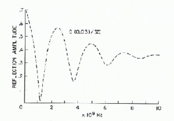
Fig. 11. Snow G (0.03 m) overeart" VI .

Fig. 12. SI/OW G (1.0 m) over earth VI.
Figure 12 shows that the difference in frequency for adjacent minima in r values is 7.4 X 10⁷ Hz, in good agreement with the value obtained from Equation (10), which is 7.38 X 10⁷ Hz. The effect of attenuation in the snow is evident from the change in values of the minima.
Discussion
The illustrative models presented in this paper indicate that snow layering affects the reflection magnitudes of EM waves as follows:
1. For the first minimum, the magnitude and frequency are substantially independent of the layer sequence, or the introduction of measureable loss in the snow.
2. Higher-order minima are quite d ependent on the d etails of the model.
The calculation of the parameters of an unknown model from the frequency variation of the r values (i.e. the "inverse problem") is not within the scope of the present paper, which is limited to the presentation of curves of r against] for illustrative models.
A few comments may be appropriate regarding limitations arising from practical matters. In this context, target characteristics such as size and smoothness may be of concern.
For specular reflection, most of the returned wave comes from the first Fresnel zone, whose area is
where H is the aircraft altitude and λ. is the transmitted wavelength. For a single homogeneous snow layer, the first dip in the plot of r against] plot occurs at a wavelength that is four times the snow thickness multiplied by the square root of the relative dielectric permittivity. For given layered media, one may use an effective dielectric permittivity given by
where hi and Ki are the layer thicknesses and relative dielectric permittivities, respectively.
As an example, if we assume that a h elicopter is at an altitude H of ISO m, and that the snow has a depth of 2 m with an effective relative dielectric permittivity of 2, the Fresnel zone area is about 2 500 m2. The free-space wavelength for the first minimum in this case is 11.3 m . If we employ the criterion that the roughness should be less than 0.1 λ., then underbrush, boulders, etc., sh ould have a characteristic dimen sion of about I m or less. Even in mountainous regions, there appear to be many locations that satisfY these requirements.
In a practical system, the matter of target characteristics must be analyzed more completely than given in this order-of-magnitude evaluation. For example, the slopes inherent in the various objects contributing to the roughness may be more important than the amplitude of the scatterers.
The remote sensing of snow-pack characteristics, with a surface-located automatic electromagnetic station may provide information regarding depth, density (from the relative dielectric permittivity) , and wetness of the snow. The target area can , of course, be properly prepared with regard to smoothness and the electrical p arameters for the earth measured directly when the snow data are being obtained. Such a system would have the important advantage that the snow pack could be monitored as often as desired , without disturba nce to the snow itself.


