


Introduction
Boundary conditions at the base of an ice mass are a subject of much interest and intense debate among glaciologists and glacial geologists. Much of the debate is centered around the velocity at the bed of a temperate glacier – whether it is a clean sliding surface or active subsole drift – and the relation of this velocity to conditions of stress and water pressure. There is generally little debate about the velocity at the bed of an ice mass whose basal temperature is below freezing – it is zero, debris or no debris.
In the present paper we describe observations made in a tunnel at the base of sub-polar Urumqi Glacier No. 1, China. In this tunnel, we have observed directly the sliding of ice over a rock surface and the enhanced deformation of an ice-laden debris layer at the base of the glacier, both occurring at sub-freezing temperatures. Two modes of deformation in the basal drift were observed, one being the deformation of the ice-laden drift as a coherent continuum, and the other being slip across shear planes both in the drift and at the contact with clean ice above. These results indicate that the assumption of a zero basal velocity at subfreezing temperatures is not valid, and that, on the contrary, the majority of the overall motion of a glacier or ice sheet can be accommodated at the bed.
Background ideas
Most theoretical treatments of glacier sliding – for both temperate ice (Reference WeertmanWeertman, 1957; Reference LliboutryLliboutry, 1968; Kamb, 1979; Reference NyeNye, 1970) and of sub-freezing ice (Reference ShreveShreve, 1984) – treat the glacier bed as a clean, rigid bedrock surface. Such a glacier bed has been observed at a few localities, generally beneath ice falls (Reference Kamb and LaChapelleKamb and LaChapelle, 1964; Reference Vivian and BocquetVivian and Bocquet, 1973). However, the more commonly observed condition at the base of a temperate glacier consists of a till-like layer containing boulders, pebbles, sand, and clay (Reference Engelhardt, Engelhardt, Harrison and KambEngelhardt and others, 1978, Reference Engelhardt, Engelhardt, Kamb, Raymond and Harrison1979; Reference BoultonBoulton, 1979; Reference Boulton and JonesBoulton and Jones, 1979; Reference BrugmanBrugman, unpublished). This subglacial drift is active, as evidenced by rolling of stones in bore-hole photographs and by relatively recent fracture surfaces on angular pebbles in the drift. Generally, water is present in this drift. Reference Boulton and JonesBoulton and Jones (1979) showed that this pore water can lead to enhanced deformation of the basal layer, providing a major contribution to the overall flow of a temperate glacier. At the base of Shoestring Glacier, Mount St. Helens, Washington, Reference BrugmanBrugman (unpublished) found that an ice-laden subglacial debris layer deforms so easily that nearly all the observed surface motion is due to deformation of this layer.
Ice-laden drift has also been observed under sub-freezing conditions at the base of several deep core holes in Antarctica and Greenland, and in a tunnel at the base of Meserve Glacier, Antarctica. Reference Gow, Gow, Epstein and SheehyGow and others (1979) stated that drilling proceeded to a depth of 1.3 m below the ice–rock interface, but all attempts to retrieve the core were unsuccessful. These authors suggested that the material was unconsolidated till or gravel, possibly 5 m thick, and contained abundant clay, sand, and pebbles which could be easily incorporated into the overlying ice, Reference Herron and LangwayHerron and Langway (1979) and Reference Hansen and LangwayHansen and Langway (1966) described the dirty basal ice zone of the Camp Century core as being underlain by several meters of an ice-laden “till-like subice material”. At the base of Meserve Glacier, Reference Holdsworth and BullHoldsworth and Bull (1970) and Reference HoldsworthHoldsworth (1974) described the glacier bed as being composed of “ice-cemented rock debris, ranging in size from clay and silt to boulders one or two meters long, projecting 20 cm or more above the general level of the tunnel floor”. Reference Koerner and FisherKoerner and Fisher (1979) presented a photograph of the base of a core hole into the Ellesmere Island Ice Cap which shows “bedrock composed of loose, angular rock fragments” with 31% rock debris by weight – clearly not solid bedrock!
Thus, while clean ice–bedrock surfaces at which sliding may occur do exist, it seems that we must often accept a glacier bed beneath both temperate and polar glaciers which is composed of drift. This drift may be ice-laden or water-saturated. In the case of temperate glaciers, Reference Boulton and JonesBoulton and Jones (1979) and Reference BrugmanBrugman (unpublished) showed that pore water in this drift plays an important role in its deformation. At sub-freezing temperatures, this basal drift cannot contain significant quantities of pore water. If results on the viscosity of dilute suspensions can be extrapolated to the relatively concentrated suspensions (such as 50–70% silicates by weight in an ice matrix) found beneath glaciers, then one would predict that the effective viscosity of frozen subglacial drift would be one to several orders of magnitude higher than clean ice and, therefore, the drift would be unimportant in the flow of ice sheets and other polar (and sub-polar) ice masses. Measurements performed on ice containing fine sand substantiate this increase in effective viscosity for relatively low solids concentrations (Reference Hooke, Hooke, Dahlin and KauperHooke and others, 1972). Surface motion studies on rock glaciers by Reference HaeberliHaeberli (1985) appear to indicate that high-solid concentration ice mixtures also have a higher viscosity than pure ice.
If, on the other hand, this ice-laden basal drift deforms more easily than the overlying glacier ice, either as a continuum (in a manner similar to the enhanced deformation of the supra-bed “amber ice” layer of Reference Holdsworth and BullHoldsworth and Bull (1970) or the structured frozen soil of Reference Thompson and SaylesThompson and Sayles (1972), which appears to be softer than ice) or along discrete planes (similar to those observed by Reference BrugmanBrugman (unpublished) at 0°C in a basal debris layer), then it could play an important role in the dynamics and stability of a cold-based ice sheet or glacier. And, as pointed at by Reference HaeberliHaeberli (1981), it is likely that Pleistocene ice sheets rested on permafrost or ice-laden drift near their margins, leading to a strong dependence of their surface profiles and stability on the rheological properties of this substratum.
Direct observation at the base of glaciers has demonstrated that basal sliding at a relatively clean ice–rock interface (where it exists) can provide a major contribution to the overall motion of many temperate glaciers (Reference Kamb and LaChapelleKamb and LaChapelle, 1964; Reference Vivian and BocquetVivian and Bocquet, 1973; Reference Engelhardt, Engelhardt, Harrison and KambEngelhardt and others, 1978). One of the two key mechanisms involved in this sliding is regelation of ice past small-scale roughness in the clean bedrock surface (Reference WeertmanWeertman, 1957; Reference KambKamb, 1970; Reference NyeNye, 1970). Because this process involves melting at points of increased pressure on the bed, it has (until recently) been unanimously assumed that sliding is not possible at sub-freezing temperatures (Reference WeertmanWeertman, 1979; Reference PatersonPaterson, 1981). Observations made in tunnels at the base of cold glaciers in Greenland (Reference GoldthwaitGoldthwait, 1960; T = −11°C) and in Antarctica (Reference Holdsworth and BullHoldsworth and Bull, 1970; Reference HoldsworthHoldsworth, 1974; T = −18°C) tend to support this idea.
There are, however, two observations which indicate the possibility of sliding at a clean ice–rock interface at sub-freezing temperatures. The first is the demonstration of regelation around wires down to temperatures of −35°C by Reference Telford and TurnerTelford and Turner (1963), and Reference GilpinGilpin (1979). The second is the observation of the development of a “sliding plane” in ice samples undergoing torsion at −2.5° to −4°C in the ice-deformation experiments of Reference Kamb, Heard, Heard, Borg, Carter and RaleighKamb (1972). This sliding surface appeared as a sharp planar boundary adjacent to the toothed grips which were applying torsional shear to the sample. A marked increase in the rate of motion was observed when this “plane” was present.
Reference GilpinGilpin (1979) has explained regelation at low temperatures in terms of a liquid-like layer adjacent to a solid foreign particle in the ice, similar to that proposed by Reference FaradayFaraday (1850) at a free ice surface and present in frozen soils (Reference Anderson and MorgensternAnderson and Morgenstern, 1973). In a recent paper, Reference ShreveShreve (1984) has used the ideas of Gilpin to show that sliding of glacier ice over a bedrock surface is possible at low temperatures. Taking water flow in the viscous liquid layer into account, Shreve predicted sliding rates of 10−1 to 10−3ma−1 at temperatures of about 10−2 to 10 deg below nominal pressure melting-point. The liquid layer at the interface is predicted to be thin, 1–10 nm (although in frozen soils it has been measured to be in the order of 100 nm (Reference Anderson and MorgensternAnderson and Morgenstern, 1973)), and thus would be virtually undetectable in a macroscopic sample. In applying this theory, Shreve has assumed bedrock roughness as measured by Reference NyeNye (1970). However, since Nye measured roughness of deglaciated bedrock at relatively long wavelengths (greater than a few tens of centimeters) using a running mean over large distances, and the wavelengths controlling sliding at sub-freezing temperatures are in the order of 0.1–10 mm (Reference ShreveShreve, 1984), it is likely that the computed sliding rates may be in error. At temperatures close to melting (−2° to −5°C), this basal sliding at a clean ice–rock interface could be an important and observable contribution to the motion of a polar ice sheet and would enhance the erosive capability of such an ice mass.
So we see that a better understanding of both basal sliding and the deformation of subglacial material at cold temperatures is required for a complete description of the motion of a polar ice mass. Important to this understanding is the direct observation of processes at the base of a cold glacier.
General Description of Field Site
The glacier
Urumqi Glacier No. 1 is situated in the Tianshan Xinjiang Uygur Autonomous Region in north-western China. The glacier is the largest of several glaciers located at the headwaters of the Urumqi River, which is a major water supply for the city of Urumqi and nearby villages. Because of its hydrologic importance and relative ease of access, this glacier has seen extensive glaciological research by members of the Lanzhou Institute of Glaciology and Geocryology (LIGG). These studies include thickness measurements, mass balance, ice temperature, surface climatology, and surface velocity.
The glacier consists of two streams flowing in separate valleys which join near the terminus (Fig. 1). The smaller western glacier extends 1.9 km from its head at 4480 m to its terminus at 3800 m and is approximately 475 m wide. Maximum thickness is 139 m with a mean thickness of 80 m (Reference Songlin, Songlin, Xiansong and GuocaiQian and others, 1982). Surface slopes are generally high, with a mean slope of 19.6° and steep (30–50 °) regions near the terminus and near its head. As is commonly observed in small polar glaciers, the margin of the glacier is cliff-like. Along the center line, annual surface velocity ranges from 2.7 m a−1 to 8.9 m a−1 and summer-time speeds are slightly larger by a few per cent (Reference Zuoche, Zuoche, Yaowu and ZhangSun and others, 1982). Ice temperature at 10 m depth varies from –1° to –10°C along the center line, with the minimum occurring near the equilibrium line (Reference JiawenRen, 1982). Extrapolation of temperature profiles to the bed indicates that a small number of localized regions may be at the melting point. Winter accumulation in this cold, continental climate is small – less than 0.5 m water equivalent per year (Reference Zhang and XiaojunZhang and Wang, 1982). During the summer there is substantial melt at the lower altitudes, leading to a sub-polar type classification for this glacier.

Fig. 1. Surface-elevation map of Urumqi Glacier No. 1 in meters above sea-level, showing the position of the tunnel.
The ice tunnel
Near the terminus of the western glacier, at an elevation of 3820 m, a 70 m long ice tunnel was excavated close to the bed by members of the Tianshan Glaciological Station (Reference Zhongxiang, Zhongxiang, Wenti, Gang and GenhaiWang and others, 1982). The tunnel is 2 m high and 1.6 m wide, with a nearly horizontal floor. Since the bed of the glacier slopes inward along the axis of the tunnel, the depth of the bed below the tunnel floor increases from zero at the entrance to nearly 6 m at the tunnel head. Ice thickness above the roof also increases along the tunnel, from 10 m to 28 m. Ablation has shortened the tunnel since its original excavation. The tunnel, as it was mapped in September 1984, is shown in plan view and in vertical cross-section in Figure 2. A vertical shaft was excavated at a point about 30 m into the tunnel. This vertical shaft extends nearly 11 m from the glacier bed upward.

Fig. 2. Plan view and vertical cross-section of the tunnel in Urumqi Glacier No. 1. Locations of numbered surface and tunnel markers are shown together with the positions of deformation studies (lettered).
Ice along the tunnel ranges from clear, nearly bubble-free at a distance of about 1.5 m above the tunnel floor to ice with several thin dirt layers (~1 mm thick) composed of silt and clay, and planes of air bubbles near the bed. Although the content of fine debris in the ice increases near the bed, there does not appear to be a distinct “amber” ice layer as was found by Reference HoldsworthHoldsworth (1974) at the base of Meserve Glacier, Antarctica. The thin layers of fine debris and bubbles are generally inclined upward towards the margins at angles ranging from 6° to 18° from the horizontal, with a few inclined at angles exceeding 30°. The slope of a layer tends to steepen as the glacier margin is approached, and in many cases the inclination is greater than that of the glacier bed (which is approximately 6° upward). Many of the fine layers appear to originate at the bed of the glacier where the debris is entrained, and they extend upward into the ice with overall lengths of several meters. Smaller bubbles (≤0.5 mm) are spherical (due to surface tension effects, a finding similar to that of Reference Hudleston, Saxena and BhattacharjiHudleston (1977)), while the larger ones are elongated along the trace of the layers (approximately in the direction of maximum shear) with elongation ratios of nearly 3:1. In some layers, the larger air bubbles have axes of 1–3 mm, while other bubble trains contain cavities up to 24 mm × 10 mm × 1 mm.
Small angular stones with axes of up to 15 cm are found sparsely scattered in the ice, including a few up to 10 m above the bed. The long axes of those stones and pebbles in the lower 1.5 m of ice are generally oriented along the flow direction, parallel to bubble and fine debris bands. The ice nearest the basal debris layer contains more angular rock fragments than ice higher up but the concentration is still small. A more complete description of the ice along the tunnel, as well as a description of previous ice deformation measurements at various points in the tunnel, has been given by Reference ZhongxiangWang (1983).
There is a relatively sharp contact between the clear glacier ice above (which has a debris content of at most 1% by weight) and that material which we term the glacier bed. This contact is interrupted in places by large boulders projecting upward from the bed. Inclination of the contact is about 3–6° upward towards the margin from the horizontal. In some regions there is a definite gap (1–10 mm wide) between the basal ice and the material comprising the bed. The significance of this gap is discussed later in the paper. Behind (in the sense of ice flow) some of the larger boulders projecting into the ice, there are cavities similar to those observed by Reference HoldsworthHoldsworth (1974). However, so-called “ropy” ice is absent within these cavities.
The glacier bed
Beneath Urumqi Glacier No. 1 the bed consists of active ice-laden drift several meters thick. A solid bedrock surface was never observed along the tunnel. Samples of this ice-laden drift contain 21–39% ice by weight. The solid material has an average density of 3.25 Mg/m3 and ranges in size from boulders several tens of centimeters in diameter to clay-size particles. Figure 3 shows the results of particle-size analysis from these samples of basal drift (from Reference Zhongxiang, Zhongxiang, Wenti, Gang and GenhaiWang and others, 1982). Ice content averaged 31% by weight for these samples. The bimodal distribution is similar to that found for some glacier till and to that found by Reference BrugmanBrugman (unpublished) in her studies of a similar subglacial drift layer on the active Mount St. Helens volcano. This distribution is not characteristic of fluvial deposits and implies that the drift has its origin in glacier abrasion and internal degradation of the debris layer. Rock fragments were generally aligned with long axes sub-parallel to the ice–subglacial drift contact and direction of flow. Within the drift, ice can occur in clear lenses up to 10 cm thick and up to 1 m long, but generally it occurs as thin (<1 cm) discontinuous layers, smaller lenses, and interspersed in the rock debris, leading to a densely packed structure in which the debris fragments are in close mechanical contact with each other, as there would be if there were no interstitial ice (Fig. 4). The bed material is well consolidated with the ice acting as a cementing matrix. There appears to be no sorting within the debris (Fig. 4) and the ice content decreased only slightly with depth in the first meter. The exact depth of this basal debris layer is not known but observations in front of the glacier indicate it is greater than 2 m. There is a fairly sharp contact between clean glacier ice and the bed.

Fig. 3. Particle-size distribution of debris in ice-laden drift. Values represent averages from several different samples. Ice content 25–37% by weight.

Fig. 4. Example of ice-laden drift from location D. Ice content is 34% by weight. Note ice lenses and change in size of solid material.
Ice Movement at the Surface and in the Tunnel
The motion of markers implanted in the surface of the glacier above the tunnel (II‒VI in Figure 2) and of points in the ceiling of the tunnel (1–6 in Figure 2) was determined using standard triangulation techniques. In horizontal projection, the surface markers were generally located within 1 m of the corresponding tunnei marker. Horizontal velocity, u, taken as the average over the period 20 September–11 November 1984, is shown in Figure 5 and Table I. Probable errors are 0.3 mm/d. The direction of flow is 10–30° from the tunnel axis and the mean flow direction corresponds roughly to the direction of maximum surface slope above the tunnel. The direction of surface flow and that of the tunnel markers are generally within 5° of each other, but the differences are believed to be real, implying a change in flow azimuth with depth. As shown in column 5 of Table I, there is a decrease in velocity with depth at all points corresponding to internal deformation of the ice. However, if the magnitude of this internal deformation is compared with that obtained from a simple model for flow in an ice mass with a no-slip boundary condition at the glacier bed, and assuming a power-law-type fluid with exponent n, no longitudinal stress gradients, and a total depth corresponding to depth to the observed (or assumed) ice-drift interface, then the predicted value of the flow-law exponent is 9.0 ± 1.0. This value is much higher than seems reasonable. Although a complex stress field may be expected near the cliff-like margin, we suggest that much of the apparent error in n is due to two factors. First, the effective depth of the glacier is greater than the depth to the ice–drift contact. This would be true if the bed was deforming through some depth on the order of 1–3 m. Secondly, if there is a layer at depth which is weak (i.e. has a low viscosity factor) relative to the ice in the column above it, then the effective value of n as obtained above would be too high, as shown by Reference EchelmeyerEchelmeyer (unpublished). As will be shown in later sections, the bed is deforming through a non-zero thickness and it is relatively weak, both of which lead to the erroneous value of n found above.

Fig. 5. Ice velocity at surface (dashed vectors) and at the tunnel roof (solid vectors). Surface-strain net with axes is also shown. Velocities shown represent early September-early November average.
Table 1. Horizontal Velocity on Surface (u S), and at Tunnel Roof (u T)

In the last column of Table I, the change in surface velocity from the first month of observaiton (20 September– 20 October) to the second (20 October–11 November) is given. A similar (possibly larger) decrease was observed at the tunnel markers. There was a net accumulation of approximately 0.1 m water equivalent during the field season, hence the decrease in velocity shown in Table I would not be expected in terms of a thickness change. We believe that the negative value of Δu S is due, in part, to a decrease in air and ice temperature observed in the tunnel as described below.
In addition to the markers II–VI, a 28 m square array of four markers centered at IV was emplanted in the surface of the glacier for the purpose of determining the surface strain field following the usual method of Reference NyeNye (1959). One diagonal of the diamond (the ξ-axis) was oriented at 104°, approximately in the direction of flow, as shown in Figure 5. The components of the planar rate-of-deformation tensor,

where negative values refer to compression.
Below we require the component of

Below we will use this result together with results from the deformation of small circular marker arrays at D to define
The vertical velocity at the surface was not well resolved by the measurements. At IV, the velocity normal to the surface, v, was approximately 4.0 mm d−1 upward and
Ice Temperature
Temperature was measured in the ice and ice-laden drift at several points in the tunnel. At the locations labeled A and c in Figure 2, thermocouple junctions were placed within 5 cm horizontally and 1 cm vertically from the precise location where motion studies were conducted, and generally at a distance of 15–20 cm into the ice from the tunnel wall. At the vertical rise, D, temperature was measured at seven points along a vertical profile extending from ~0.5 m into the subglacial drift to a point 8.5 m above the ice–drift interface. Three thermistors in this vertical profile were monitored daily, together with the air temperature near marker 3 in the tunnel. All other temperature probes were monitored at 14–30 d intervals. Accuracy of the calibrated thermistor measurements was 0.04°C, while the thermocouple junctions were read to approximately 0.2°C.
The following temperatures were observed at A (in clear ice 1 cm above the clean contact with a large boulder) and at c (in ice 1 cm above the ice–drift interface):T A = −4.6°C,T C = −4.1°C.
Temperatures varied by ±0.7 deg at these sites (and at D as well). This variation was due, in part, to changes in air temperature in the tunnel. Several cold spells (−15° to −20°C) caused the air temperature to drop in the tunnel by a few degrees, as well as causing significant external cooling of the glacier.
Results of temperature measurements at D are shown in Figures 6 and 7a. Temperatures determined with a precision thermometer at several points near those in Figure 7a agree well with those shown. The profile in Figure 7a suggests that non-steady-state conditions were present in the ice near the tunnel walls. Circulation of air in the tunnel and its connection with the outside air could lead to air temperatures in the tunnel which would differ from the bulk ice temperature. With the depth of penetration of these air-temperature fluctuations, given approximately by (2k/ω)1/2 where k is the thermal diffusivity of ice and ω/2π the frequency of oscillation, daily fluctuations would be felt Strongly at a depth of 18 cm into the walls, near the depth of our measurements. It is interesting, however, that the vertical structure of this profile was maintained throughout the period of observation, as shown in Figure 6.

Fig. 6. Ice temperature at D and air temperature in tunnel near c. Location of points c and D are shown in Figure 2.

Fig. 7. Measurements made in the ice of D profile. Depth below surface and approximate shear stress are shown. (a) Temperature (lowest point is in drift). (b) Longitudinal and (c) transverse rates of deformation from strain circles. (d) Transverse shear rate and (e) shear rate in plane of tunnel wall. The x-axis is taken parallel to the mean surface along the direction of the tunnel axis and y is positive downward. Open circles in (e) are values derived from strain circles and the crosses represent averages between several markers over a shorter time period than the solid dots.
The vertical gradient near the ice–debris interface at D was 0.5 K m−1 (over 0.6 m), while the gradient over the lower 2.5 m of the profile was 0.3 K m−1. These gradients are more than an order of magnitude greater than those expected due to the geothermal heat flux (
At no location was the temperature ever greater than −1.75°C. This is well below the pressure-equilibrium temperature of pure ice and water under the pressure of 20 m of ice, and, thus, we may accurately assume that all ice and ice-laden drift discussed in the sections to follow were at a temperature below freezing and that the amount of liquid water present in the ice was insignificant (Reference HarrisonHarrison, 1972).
Temporal fluctuations of temperature are shown in Figure 6. As indicated above, there is a general decrease in temperature, apparently in response to a drop in outside air temperature. Although these variations may be local in nature due to the presence of the tunnel, it is interesting to note that the surface velocity appears to respond to this decrease in local ice temperature. One would expect the velocity to be related to the bulk ice properties rather than local conditions in the tunnel. Similar anomalous results were found by Reference HoldsworthHoldsworth (1974) in the Meserve Glacier tunnel, where, at a point 40 m into the tunnel, a 12% decrease in speed appeared to be related to a 7 deg drop in outside air temperature.
Observation of Sliding at an Ice–Rock Interface
Few locations along the tunnel were amenable to the direct measurement of the sliding of clear glacier ice over a relatively clean rock surface as is assumed in the theoretical treatment of Reference ShreveShreve (1984). One such location was approximately 5.2 m into the tunnel (designated A in Figure 2), where the thickness of ice above the tunnel floor was approximately 14 m and the mean ice temperature at the point of measurement was −4.6°C during the period of observation. A large boulder (~35 cm along the plane of flow, 22 cm thick at the tunnel wall, increasing to ~50 cm thick at a point in from the tunnel wall, and at least 100 cm in length) extended inward from the tunnel wall approximately transverse to the flow direction. The boulder was embedded in the ice-laden drift below and protruded up to 15 cm into the ice above (see Fig. 8). On the down-stream side of the boulder there was a cavity.

Fig. 8. Sliding interface and instrumental set up at sliding point A. (a) Overall view of boulder, bubble, and debris trains in ice and dial gauge on marker in ice. Displacement transducer was attached below the gauge on the same anchor. (b) The sliding interface at the surface of the boulder. The actual interface was much cleaner than that shown. The transducer core was attached to the boulder directly below the marker in the ice.
The composition of the boulder was gneissic, and the edges were rounded and surfaces smooth. A few thin bands of fine debris appeared to originate at the surface of the boulder, where the rock flour was entrained, and they extended 1–2 m upward into the ice at 14–18°. On a macroscopic scale, the glacier ice did not appear to vary from the tunnel roof to the ice–rock interface, except for the slight increase in debris and bubble content found elsewhere along the tunnel.
The sliding measurements described here are relative measurements between the boulder and the ice. The boulder itself was not fixed in space but rather embedded in the sub-glacier drift, which was itself in motion. Absolute velocity of the boulder was about 5 mm d−1 and surface velocity above A was about 10 mm d−1 during the same period. The boulder did not rotate measurably during the time of observation.
A small wooden stake, designated AI and 6 mm in cross-section, was driven into a hole drilled into the ice just above the ice–rock interface. The lower face of the stake was less than 1 mm above the rock at the tunnel wall and was in direct contact with the boulder in from the wall at a distance of about 9 cm. Abrasion of the lower surface of this marker was observed at the end of the experiment, indicating that there was indeed relative motion between marker and rock.
Displacement of the marker was measured daily using precision dial gauges. Results indicate that the motion was directed out from the tunnel wall at this point (128°). The stand holding the dial gauge was anchored to the ice-laden drift approximately 30 cm below the stake. Because of the deformable nature of the drift, this stand also had a small (1.5mm d−1) component of motion as well.
Motion of the boulder (AR) was determined by two means. The method used initially, and the least accurate, involved measuring the distance between two points, one on the rock just below AI, and the other on a peg driven into the drift near the base of the stand holding the dial gauges. A comparison of speeds determined by this same method for the marker in the ice, AI, shows good agreement with the dial-gauge results averaged over the same time periods.
The second method employed a 24 V displacement transducer affixed to the same stand as the dial gauges. The movable core of the transducer was attached to the boulder just below the ice–rock interface via a short length of fine cable fixed in place by epoxy resin. Both excitation and signal voltage were measured with a resulting accuracy of ±0.01 mm. Since the sliding measurements were to be based on a comparison between dial gauge and displacement transducer, comparative calibrations were made during the observation period by using both methods to measure the displacement of AI.
The results of the sliding measurements are shown in Figure 9. The marker in the ice (AI) moves at a speed consistently greater than the boulder (AR). The two points show roughly the same temporal fluctuations. There is an overall drop in speed in November, similar in timing and relative magnitude to those observed at the surface and tunnel roof as described above and, again, corresponding to a drop in air temperature. The ice temperature at A was −3.9°C on 22 October and dropped to −5.1°C on 4 November, about the time of the drop in speed at AI.

Fig. 9. Observed motion at sliding point A. AI signifies the ice, AR the boulder. The difference in speed is interpreted as sliding along the interface. Representative error bars are shown together with periods of calibration.
The difference in velocity between the ice and the boulder is interpreted as a sliding velocity. Based on the earlier method of measurement, the mean sliding speed is 0.45 ± 0.11 mm d−1, while that obtained using the transducer is 0.48 ± 0.17 mm d−1. (The plus/minus values indicate the standard deviation of the velocity about the mean and not an estimate of standard error in the sliding speed which is, formally, 0.22 mm d−1 and 0.05 mm d−1 for the initial and transducer methods, respectively.)
The sliding speed of 0.5 mm d−1 is roughly 5% of the surface speed and thus represents only a small fraction of the overall motion. However, over a period of many years this sliding motion can amount to several meters and thus contribute to glacier abrasion. A similar relative contribution of sliding to the overall motion of some temperate glaciers has been observed (e.g. Reference EchelmeyerEchelmeyer, unpublished).
A comparison of the observed sliding speed with that predicted by Reference ShreveShreve (1984) may be made. The approximate sliding speed is given by

(Reference ShreveShreve, 1984, equation (14)) where, following the notation of Reference NyeNye (1970), a is a measure of surface roughness, k 0 is a critical wave number, ƞ i is the viscosity of the basal ice, and ˂τ xy ˃ the basal drag (taken equal to the basal shear stress), Using the values of the fundamental parameters listed by Shreve, computing k 0 by his equation (11) and using the value of a = 0.022 as measured by Reference NyeNye (1970), we determine a sliding velocity of 0.002−0.01 mm d−1 at −4°C under shear-stress conditions appropriate to the base of the glacier at A (shear stress 40–70 kPa (0.4–0.7 bar)).
These predicted sliding speeds are nearly two orders of magnitude below those observed. The treatment of Reference ShreveShreve (1984) allows for the presence of dissolved impurities in the thin (a few nm thick) liquid layer but these solutes (even at concentrations of up to 104 ppm) do not increase the sliding speeds a great deal at these temperatures (a doubling at most). The sliding velocity calculated above assumes a flow-law exponent equal to 3 in determining the effective viscosity. This value and the corresponding viscosity factor are not well constrained but, again, changing the value of n does not change the sliding speed significantly.
The parameter in Equation (2), which is the least well-known, is the roughness parameter, a. Its value was determined by Reference NyeNye (1970) from recently degtaciated bedrock in Norway. Nye used simple running means over 61–122 m along a profile 244 mm in length. Although not stated explicitly in Nye’s paper, it is unlikely that measurements were made on a small enough scale that the computed value of a can be considered applicable to wavelengths on the order of 1 cm. On the other hand, Reference ShreveShreve (1984) showed that knowledge of the roughness at wavelengths 0.1–10mm is required at sub-freezing temperatures, since 90% of the drag comes from bedrock roughness at these wavelengths.
We have measured the roughness of a sample which is similar in roughness to the boulder at A (the sample was taken from a nearby location at the bed). The amplitude of surface topography was determined using a precision dial gauge moving across the surface (read every 0.25 mm across a 70 mm profile). The observed topography was smoothed using a simple centered mean and the root-mean-square deviation from this smoothed surface was computed using several averaging lengths, X av, leading to several values of the “roughness” r = r.m.s. deviation/X av; Reference NyeNye, 1970, equation (7)). The parameter a (= 4πr 2/0. 148; Reference NyeNye, 1970, equation (13)) is given below for representative X av :

These different values of a were determined over the same sample length. If, as assumed by Nye, “the glacier bed looks the same when viewed on different scales”, then one would expect a to be independent of scale x av. Nye found this to be true for deglaciated bedrock at large scales (100 m) but, as is shown above, it appears that this assumption is not valid at the shorter wavelengths important in sliding at cold temperatures. In order to describe more accurately sliding at low temperatures, it would be best to use the more complete sliding theory using spectral information at each wavelength (Reference KambKamb, 1970; Reference NyeNye, 1970). However, this is not done in the present paper. Instead, we take the mean value of a as listed above to be a representative value for shorter wavelengths. This mean is
Using the mean value of a (assumed constant), we find predicted sliding speeds of 0.01–0.06 mm d−1 from Equation (2). Although closer to the observed values, these speeds are still low by an order of magnitude.
Following the motion studies at A, a column of ice was removed for ice texture and qualitative fabric analysis, and inspection of the sliding interface. The ice was firmly frozen to the boulder’s surface and was extremely difficult to remove, even with application of some heat. This indicates that any liquid regelation layer present must be very thin and refreeze rapidly and solidly upon release of the overburden.
The physical properties of the ice column will be described in detail below but we note here that over much of the surface of the boulder there appears to be a thin (˂1–2 mm) layer of fine rock flour and small oriented rock fragments interbedded with thin ice layers forming five to six thin laminae as shown in Figure 19. The presence of this 1 mm layer may effectively smooth the ice–rock interface and, in addition, the layer itself may be significantly more deformable than the bulk ice. The properties of this thin layer at the interface may therefore be important in determining the sliding speed.

Fig. 19. (a) Vertical thin section taken near the sliding interface at A showing the thin debris layer at the interface. The debris layer was nearly continuous along the interface below this sample. (b) Detailed view of the interfacial debris layer showing thin, alternating laminae of debris-rich ice and relatively clean ice. Division of scales is in mm. Ice motion is in the plane from left to right.
Deformation of Ice-Laden Subglacial Drift as a Continuum
A profile of 30 markers over vertical extent of approximately 11 m allowed the rheological properties of the ice and ice-laden subglacial drift to be investigated at location D, approximately 40 m into the tunnel. The vertical profile extended from nearly 0.5 m into the debris upward through approximately one-half of the total thickness of the glacier at this point. In order to reach the glacier bed, the vertical shaft dropped 3.5 m below the tunnel floor. The entire shaft was excavated by members of LIGG in 1983 and 1984. The wall of the shaft was oriented at approximately 20° from the observed flow direction.
Wooden markers (2 cm diameter) were driven into holes drilled in the shaft wall at about 0.5 m spacing from the top of the shaft down a distance of approximately 10 m. These markers are designated D0 (top) to D19 (at 9.75 m). Points D20 to D23 were smaller-diameter (7 mm) wooden markers placed at a reduced spacing, with D23 3 cm below the ice–drift contact (see Fig. 7).
Deformation of the originally vertical profile, D0–D23, was determined over a period of about 2 months using plumb lines. (The deformation of the profile defined by the upper 15 markers was also determined over a longer time period.) In addition, five initially circular arrays of markers were placed in the wall at D in the upper 6.5 m, designated DI to Dv from top to bottom, respectively. Deformation of these circular arrays over a period of nearly 11 months allowed determination of strain ellipses in the plane of the tunnel wall at various depths.
The remaining markers (DA–Df) were small wooden pegs or nails placed within or just above the subglacial drift (Figs 11 and 12). Displacement of these markers was accurately determined over daily intervals using precision dial gauges and displacement transducers. Space limitations did not allow the motion of all markers DA–DF to be followed at one time, but there is sufficient overlap to allow a complete description of the deformation field. As with the sliding measurements at A, the base of the platform holding the gauges and transducers was possibly within the active part of the subglacial debris and, therefore, only relative motion could be determined.

Fig. 11. Photograph showing markers in ice-laden drift at D. Motion is roughly in the plane of the photograph from right to left. The upper pencil marker is D22, the lower D23, the upper nail is DA, and the lower one is DB.

Fig. 12. Diagrams of marker placement above and in the ice-laden drift at the base of D profile. D22 and D23 are the lowermost points of the deformation profile extending up into the ice (Fig. 7), Distance shown is that below ice/drift (I/D) contact. The anchoring point for displacement transducers was re-set from the location shown in (a) to a greater depth in the drift (b) on 8 October. Ice motion was from right to left in the figure.
We will discuss the deformation of the bulk ice (D0 to D23 and the strain circles) first. This then allows a comparison with results from the markers in the ice-laden drift.
Principal strain-rates and directions were obtained by semi-graphical means for the circular arrays. These are given in Table II. The rate of deformation,
Table II. Principal Axes of Strain Ellipses

There is a linear variation of
The gradient of
The linear variation of
for a depth below 10 m. This result is similar in sign to that found by Reference HarrisonHarrison (1975) and Reference PatersonPaterson (1976) but, as found with
If plane-strain conditions existed at D, then incompressibility would require

obtained by integration of the general equation for bore-hole tilt (Reference RaymondRaymond, 197l[b], equation (9)) over the finite time interval [0,t 1] and assuming an initially straight profile,
In order to estimate the rheological properties of the ice from these deformation measurements, we require the shear stress,
where ρ is the density at ice, g the acceleration of gravity, f a channel-shape factor, and ˂fHsin α˃ represents an appropriate average of f, ice thickness H, and surface slope α (see Reference Kamb and EchelmeyerKamb and Echelmeyer, 1986). This linear relation will be only approximate in the vicinity of the ice cliff and away from the channel center line (Reference EchelmeyerEchelmeyer, unpublished). A more accurate estimate of shear stress would be obtained by making a finite-element analysis of the stress field within the complex glacier geometry, but in the present calculations we use Equation (6), with f = 1. This approximation will still allow an accurate assessment of the relative rheology between the ice and the underlying drift.
The rate-of-deformation component
We require an estimate of the ice-flow properties as a function of depth for comparison with those of the basal layers. This is obtained from Figure 10 which shows a logarithmic plot of

Fig. 10. Logarithmic plot of
The placement of markers DA–DF in the layer of basal drift is shown in Figures 11 and 12. Locally, the ice–drift interface dipped steeply (42°) to the south (174°), while the dip along the wall direction (100°) was 12°. This local topography may give rise to a divergence of the flow direction relative to the azimuth observed at the surface. At a distance of 1–1½ m above the bed there were thin layers of fine debris sloping upward towards the east at 50°. The ice-laden drift at DB and DD contained 38% ice by weight. There were no observable planes of discontinuity in the vertical deformation profile, either at the ice–drift contact or within the drift itself. Therefore, we treat the drift as a continuous medium.
Displacement at the points in and just above the debris is shown in Figure 13. These displacements are relative to the anchoring point of the instruments which was itself in motion before being re-set to a deeper position in the drift. The large increase in speed, of DB and D23 following 8 October was caused by a re-setting of the anchor point some 215 mm lower, from a depth where the drift was deforming to a depth where it appeared inactive. The resetting on 30 October had little effect on the measured speeds, indicating that the absolute motion of the anchor at its lower positions was nearly zero.
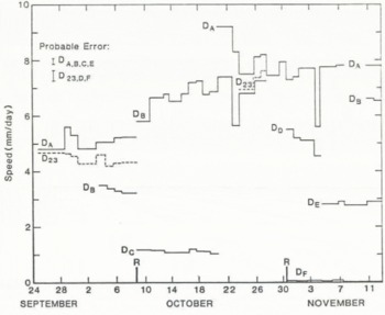
Fig. 13. Motion of markers in and just above the drift at d. Re-setting of the anchor point is shown by r.
There are significant fluctuations in speed at all points. In some cases, these variations are synchronous among the different markers, while in other cases there is little correlation, especially over shorter (~1 d) time intervals when the probable errors are larger.
The motion of DA was approximately 8 mm d−1 relative to the base. This speed is seen to be approximately 60% of the surface speed, showing that most of the motion of the glacier at this point is contributed by deformation of the ice-laden glacier bed which has an active layer thickness of about 0.35 m – or less than 2% of the total thickness of the glacier.
The shear-deformation rate was calculated from the data shown in Figure 13 using
It was found that the resulting values of
Results based on this position of the effective bed are shown in Figure 14. Comparison of Figures 7e and 14 shows two things: (1) the rate of shear deformation in the drift is much larger than that in the overlying ice, and (2) the increase in

where

Fig. 14.
The internal deformation of the drift itself shows a strong variation with depth. The effective value of the stress exponent, n, in a power-law type constitutive relation is much greater in the drift than in the ice.
While we do not feel that the actual flow law of the subglacial drift can be determined from the above results because of the complex geometry of the local stress field and the small variation in overall shear stress, we do believe that the observations definitely show a marked decrease (on the order of 100-fold or more) in the creep strength (ηeff) of the drift relative to pure ice at a similar temperature under an equivalent stress level. Even if higher shear stress occurs near the margin of the glacier because of the (possible) presence of warm ice and water-saturated drift under the deeper central glacier (Reference HaeberliHaeberli, 1981), it is highly unlikely that the shear stress in the drift and that in the adjacent clean ice at D will differ substantially. Thus, the relative viscosity of these two media as determined here should remain valid even if there are zones of weaker substrata.
The finding that the effective viscosity of the frozen subglacial drift is much lower than that of the overlying ice has profound implications in the flow of major cold-based ice sheets. But how do we explain these results? If free pore water were present, then deformation mechanisms similar to those described for saturated deformable media would apply and a decrease in viscosity would be expected. This is the basis of the results described by Reference Boulton and JonesBoulton and Jones (1979) and Reference BrugmanBrugman (unpublished). Temperatures in the present case preclude liquid pore water in large quantities and we must therefore appeal to other mechanisms.
The ice-laden drift could be considered as a suspension of particles in a viscous fluid. Most theoretical and observational rheological studies of dilute to moderately concentrated suspensions of rigid particles in a viscous fluid (Reference EinsteinEinstein, 1906; Reference RoscoeRoscoe, 1952; Reference ChongChong and others, 1971) show that the viscosity of a suspension is greater than the pure fluid and increases with the volume concentration of particles. This is a direct consequence of the disturbed flow created by the particles, which leads to an increase in energy dissipation. If the particles are of uniform size, the viscosity of the suspension is higher than if there is a distribution of particle sizes (such as found in the subglacial drift), but for all particle-size distributions the viscosity is greater than that of the ambient fluid. There is some critical volume concentration (~0.6) at which the suspended particles form an interlocking structure and the material no longer behaves as a fluid of finite viscosity. Theoretical studies generally assume that there is a no-slip boundary condition at the solid inclusion–liquid interface. If, however, there is slip, then the flow disturbance will be less and there will be a lower rate of energy dissipation than in the no-slip case. Such slip could occur by regelation sliding in ice at temperatures near melting (T ˃ −3°C). This will lead to decrease in the ratio of the effective viscosity of the suspension to the ambient ice, although one would still expect the ratio to be greater than one, and thus the drift would be stiffer than pure ice.
Deformable solids with dispersed solid inclusions show similar increases in effective viscosity. The solid inclusions can act as pinning points for dislocations, inhibiting their propagation. Silicate inclusions in ice at sub-freezing temperatures lead to dispersion hardening when the fraction of inclusions is small (Reference Hooke, Hooke, Dahlin and KauperHooke and others, 1972; Reference Baker and GerberichBaker and Gerberich, 1979), giving a substantial increase in creep activation energy and a large increase in effective viscosity at cold temperatures.
The above results are generally found for relatively low concentrations of solids. When the volume concentration of solid inclusions exceeds about 0.6 (as is the case for the drift) the solid–solid interactions in the medium must be taken into account. Observations indicate that the properties of granular materials are useful in describing the deformation of these dense suspensions (as summarized by Reference Cheng and RichmondCheng and Richmond (1978)). Examples of this granulo-viscous behavior include dilitation, liquefaction, flocculation, and the development of “slip planes”. Since the ice-laden drift contains a large volume concentration of rock particles which range in size from clay to boulders, it is likely that some of these granuloviscous effects are important in its deformation. Indeed, slip planes do occur in the drift at some locations (as described in the following section) but macroscopic slip planes were not observed at D.
In many respects, the ice-laden drift is similar to permafrost or the interior of a rock glacier. Several experimental studies on the rheological properties of permafrost have been undertaken and, based on these results, it is often stated that frozen ground is less deformable than ice itself under similar conditions (although there have been few in-situ comparisons). For purposes of comparison, we have taken the power-law type flow relation obtained by Reference HaynesHaynes (1978) with n ≈ 3 from compression experiments on frozen silt at rates of deformation exceeding 10−4s−1 at −2° C and extrapolated to the stress–temperature conditions within the drift at D. With a shear stress of 57.5 kPa, we find a predicted rate of deformation equal to 45 × 10−9s−2 Considering the large range of extrapolation in stress (and creep rate), this agrees quite favorably with the observed value of
In-situ creep measurements in frozen structured soil (low volume concentration of ice) performed by Reference Thompson and SaylesThompson and Sayles (1972) also indicate a power-law constitutive relation. They found that permafrost may deform at a faster rate than polycrystalline ice at an equivalent stress level and temperature.
Reference HaeberliHaeberli (1985) has given a thorough discussion of the motion of rock glaciers. Except for the near-surface layer of boulders and the presence of several large ice lenses, the general characteristics of the material comprising the rock glaciers studied are similar to those of the drift under Urumqi Glacier – both in ice content and solid-particle size distribution. In contrast to the results presented here and to those of Reference Thompson and SaylesThompson and Sayles (1972), Haeberli found that the creep rate of these rock glaciers (at T = −1°C) was at least one order of magnitude less than that expected for pure ice. However, the shear stress used in that study may have been overestimated. In any case, no direct observational comparison was made with clear ice under similar conditions.
The mechanisms of deformation for permafrost, rock glaciers, and the subglacial drift will be similar. Important to these mechanisms is the presence of a thin (6–10 Å) layer of liquid water surrounding each soil particle down to low temperatures (–100°C). This layer has been described by Reference Anderson and MorgensternAnderton and Morgenstern (1973). Nearly perfect slip could occur at ice–particle and particle–particle interfaces if this layer were continuous enough. This could then lead to a significant decrease in effective viscosity of the bulk material. Intergranular friction between soil grains, and between soil and ice grains, may also be important as a granulo-viscous effect (Reference Sayles and HainesSayles and Haines, 1974). This internal friction may allow failure of the Mohr–Coulomb type to occur within the drift and, possibly, lead to the development of the shear planes described in the next section.
Motion Across Discrete Slip Planes
In addition to the spatially continuous deformation of ice and ice-laden drift described in the previous section, we have also observed discontinuous profiles of deformation at two other locations, designated B and c in Figure 2. Significant slip was measured across well-defined “shear planes” or “slip planes”, with little deformation of the medium between planes. One “plane” was along the ice-drift contact, while others were observed within the ice-laden drift.
The photographs in Figure 15 show the ice–drift contact at location c and the instrumental set up. The interface between clean ice and the underlying debris (32% ice by weight) was sharp and, for the most part, there was intimate contact between the two media. At a few points along the interface there were slight air gaps 1–5 mm in breath, but in a neighborhood of length 40 cm or more about the point of measurement no such gap existed. The overburden stress at the contact was about 142 kPa (above atmospheric) and the shear stress was about 46 kPa.

Fig. 15. (a) Instrumental set-up at the base of the tunnel at c showing the displacement transducer attached to a marker at the shear plane. Large peg (c4) is about 17 cm above the shear plane, (b) Close-up of the shear plane showing the sharp boundary between clean ice and drift. The furthest above the plane is c5, that below the plane is c7. The nail head is about 5 mm in diameter.
The motion of the large peg c4 (set in clean ice 180 mm above the contact) was measured using one or, at times, an orthogonal pair of dial gauges. c5 through c8 (see Figure 16a) were small-diameter (1.5 mm) nails whose displacement was determined using a displacement transducer. Along the tunnel wall above c4, three additional markers with 0.5 m spacing allowed deformation within the bulk ice to be determined.

Fig. 16. Location of markers relative to the ice-drift contact (a) at c (depth below surface), and (b) at b, b1 is approximately 12 m below the surface.
Absolute motion of c4 was approximately 10 mm d−1 during the period of observation, while the anchoring point for the instruments, which was about 170 mm below the ice–debris contact, was moving at a speed of nearly 6 mm d−1.
Results of the displacement measurements at c4 to c8 are shown in Figure 17. Effective rates of shear are shown in Table III for the deformation across the plane and in the overlying ice. These shear rates are extremely high (up to 40 a−1 or 1.3 × 10⁻⁶ s −1), while those in the ice are similar to those observed in the ice at D.

Fig. 17. Motion of markers at c near the shear plane (see inset in Figure 16a). Representative error bars are shown. The anchor was re-set to a slightly greater depth at the time denoted r.
The ice-drift contact between c6 and c7,8 appeared to be a definite slip plane when viewed over a period of a few days and the velocity results shown in Figure 17 and Table III support this observation. A slip rate of approximately 1.25 mm d−1 occurred across this plane, amounting to 10% of the surface motion. Much of the remaining motion was contributed by deformation of the drift below the contact. No other definite shear planes were observed in the debris below the ice contact.
Table III. Effective
Another vertical profile of markers was established at location B (Fig. 2), extending from 20 cm above the ice–drift interface downward to a depth of 70 cm into the debris, as shown in Figures 16b and 18. Within the drift there were several relatively ice-rich layers overlying a debris-rich substratum. Approximately 20 cm below the uppermost point (B1) there was a 2–4 cm thick debris band which appeared to contain little ice (Fig. 18b). A slip rate of up to 2.5 mm d−1 was measured across this layer (25% of the surface motion). Above and below this region, the ice and ice-laden drift appeared to deform more or less continuously except for a zone in the lower 15 cm of the profile where one other shear band or plane developed in the ice-depleted drift. Quantitative measurements were not made across this lower zone but its presence is apparent in the large value of the effective rate of shear deformation from B5 to B6 shown in Table III.

Fig. 18. (a) Deformation profile at B showing interlayering of ice-laden drift and relatively debris-poor ice. The profile was originally vertical. Plumb line is attached to B1. (b) Close-up of debris in shear zone between B2 (peg) and B3 (small rock). Shear zone is approximately 4 cm across.
The zones of intense shear at B were not as narrow as that found at C. We term the 10–25 mm wide zones at B “shear bands”, while the discontinuity found at the ice–drift contact at C is a “shear plane”. Shear bands appear to be layers of ice-poor debris separating regions of clean ice and/or debris-rich ice.
Shear bands consisting of water-saturated debris up to 10 cm thick have been observed by Reference BrugmanBrugman (unpublished) within Shoestring Glacier, Washington, and by one of the present authors along the surge front of Variegated Glacier, Alaska. In both cases, there was a large relative displacement between upper and lower faces of the band due to intense deformation of the debris layer. Reference BrugmanBrugman (unpublished) has given further discussion of the properties of these shear bands, where high pore-water content (and pressures) in the debris is found to be important in their development on the temperate Shoestring Glacier. Such liquid water is not present in the shear bands described here but, as shown in the previous section, ice-laden debris could form a layer of reduced creep strength relative to the surrounding ice, leading to a shear band.
The shear bands and planes observed here and elsewhere allow 10–25% of the total ice motion to occur over 0.01–0.1% of the total ice thickness and, as seen at B, more than one such band may occur. Combination of these shear planes or bands with the enhanced deformation of a basal continuum of drift may well account for 80% of the motion of a cold glacier – all in less than a few per cent of the total thickness!
Fabric and Texture Analysis
Samples of ice were removed from the tunnel wall near A, B, and D in order to investigate crystallographic properties at the sites where different types of motion were observed. About 44 thin sections were made on which crystal-size measurements and qualitative fabric analyses were performed. In this section we briefly describe the overall results and then give a detailed description of the ice directly adjacent to the sliding interface at A and the shear plane at C.
Mean crystal size (as determined by grain-boundary counts across the sample) generally shows a gradual decrease with depth from 1.5–2.0cm at 10 m above the bed down to 0.3–0.4 cm near the ice–drift interface. A fabric with a strong single maximum in c-axis orientation normal to the plane of maximum shear develops as the bed is approached (the stress level increases and grain-size decreases). These findings are similar to those observed in polar ice by Reference AndertonAnderton (1974), Reference Hooke and HudlestonHooke and Hudleston (1980), and Reference HudlestonHudleston (1980). Some studies on temperate glaciers (Reference QuintanaQuintana, unpublished) have found a similar relation with shear stress but with coarser-grained ice showing the stronger fabric at higher stress levels. Several extremely strong single-maximum fabrics were observed within 5 cm of the boulder at A and the ice–drift contact at C, but at other nearby locations the fabric did not show a strong preferred orientation. It therefore appears that, in the vicinity of the uneven bed, flow perturbations cause local changes in fabric and texture, similar to the findings of Reference AndertonAnderton (1974).
It is generally believed that strong simple shear rates produce a fabric with a single maximum, where the c-axis is normal to the local shear plane (Reference Hooke and HudlestonHooke and Hudleston, 1980; Reference HudlestonHudleston, 1980; Reference QuintanaQuintana, unpublished). With the observed deformation profiles described in earlier sections of this paper, one might not expect the development of such strong fabrics at locations such as A and C because much of the shear strain is concentrated at and beneath the ice–drift interface, with relatively little ice deformation above it. It may be, however, that sufficient strain above the interface is accumulated over a period of time. On the other hand, the presence of these strong fabrics may indicate that there are zones of concentrated ice deformation at some locations up-glacier of the tunnel and further away from the margin. These fabrics may then be relics carried in to the tunnel region.
With some difficulty, ice samples were obtained directly from the sliding interface on the boulder at A. The grain-size in these samples showed no consistent trend over the lowermost 5 cm. However, detailed observation of the actual ice–rock contact often revealed a thin debris-laden zone which ranged from 0.5 to 4 mm in thickness. This zone (shown in Figure 19) consisted of laminae of fine clay and silt and small elongated rock fragments aligned parallel to the rock surface. These debris-laden bands were interlayered with clear ice bands, forming a laminated structure with approximately four laminae per millimeter, all of which were parallel to the interface. Above this zone there was sometimes a 1–2 mm thick band of very fine-grained ice (<½ mm grain-size), while in other places nearby the larger grains of the ice above would extend up to and, at times, into the debris–ice laminations. The parallelism of these laminae with the surface of the boulder indicates that they may have an origin associated with sliding at the interface.
From the results of several sections above, we see that the creep strength of this thin, debris-laden interfacial layer could be significantly reduced from that of clean ice. Since the effective viscosity of this layer will govern the sliding speed, the calculations based on Equation (4) are likely to be in error. From the above, we may take a viscosity 100 times smaller for the interfacial layer. This would lead to an increase in predicted speed of about 22 times, which greatly improves the agreement with the observed rate of sliding.
Additional ice samples were taken directly from the point-of-deformation measurement at C, extending into the drift. Thin sections parallel to the shear plane (Fig. 20) and 2–5 cm above it show (qualitatively) a strong single-maximum fabric normal to the interface. At the ice–drift contact, there was commonly a thin (4–10 mm) band of very fine-grained ice (<½ mm), as shown in Figure 20, but such a layer was not universal. This layer often had a high bubble content and thus it may have had its origin as fractured ice contained in a small gap at the shear plane. The ice–drift contact itself was sharp and well defined with no penetration of clean ice into the ice-laden drift. This clearly defines a plane of discontinuity between the ice and the underlying drift.

Fig. 20. Thin section taken vertically just above the shear plane at c showing the fine-grained ice layer near the interface. The upper boundary of this layer was distinct and non-gradational. The base of this sample corresponds to the position of c5–c6. Ice motion was roughly in the plane from left to right.
Within the drift itself, ice was found in two different types of structure, the first being small, coherent ice lenses up to 2 cm wide and 20 cm long, and the other being within very debris-rich material, where ice was often found distributed in fine laminae (at most a few millimeters thick) or in the intergranular spaces of the debris matrix. Ice in the lenses was fairly coarse (2–6 mm) and no strongly preferred orientation of the grains was observed. Mean grain-size within the thin laminae was approximately 0.5 mm. The ice lenses were aligned in the flow direction but were highly discontinuous. It appears from these results that most of the deformation of the drift was occurring within the regions of high debris content and not in the ice lenses, although no fabric analyses were made on the ice in the thin debris-rich bands.
Conclusions
Direct observation in a tunnel at the base of sub-polar Urumqi Glacier No. 1 has shown that there are three mechanisms of flow which, either singly or in combination, can contribute nearly all (70% or more) of the overall motion of a cold-based glacier. These three mechanisms act in the lowermost 1 or 2% of the effective glacier thickness. All three have previously been considered to be negligible or non-existent in the motion of cold ice masses.
The three modes of flow are basal sliding, deformation of subglacial debris, and motion across shear planes or shear bands within the subglacial drift.
Basal sliding at sub-freezing temperatures has only recently been discussed theoretically (Reference ShreveShreve, 1984). The findings of this theoretical work are that sliding rates, while significant in terms of long-term glacier erosion, are quite small and that the rate of sliding by regelation in a thin water film is governed by roughness at wavelengths of 0.1–10 mm. Roughness measurements at these short wavelengths did not previously exist for accurate predictions of sliding speed but estimates of speed were about 0.01 mm d−1 at temperatures of 5 deg below freezing.
We have measured sliding rates of 0.5 mm d−1 over a solid rock surface at a temperature of −4.6°C under a shear stress of approximately 60 kPa. While small, this rate is much greater than that predicted by Reference ShreveShreve (1984) using a measure of roughness made at long wavelengths. Measurement of the actual roughness at the shorter wavelengths on the actual sliding surface indicates that a glaciated bedrock surface can be five to ten times smoother than it is at longer wavelengths. This smooth surface allows increased sliding but predicted values still fall short of those observed. The presence of a thin (1–2 mm) layer of low-viscosity, fine debris-laden ice at the sliding interface may contribute to the observed increase in sliding speed above that derived from the sliding theory. Errors in the effective shear stress at the bed may also contribute to this discrepancy.
As many cold-based glaciers are underlain not by a clean bedrock surface but instead by a layer of ice-laden subglacial drift, the question of basal sliding may not be as important as that concerning the deformation of this subglacial drift. Observation of the deformation of the glacier bed at a temperature of about −2°C indicates that ice-laden drift forms a weak substratum beneath the glacier. A significant contribution (60%) of the overall surface motion is provided by deformation of a layer of basal drift 35 cm in depth (<2% of the total thickness). The effective viscosity of this subglacial drift is more than two orders of magnitude less than the overlying ice and it appears to be very non-linear in its rheologic properties. The presence of a liquid-like layer surrounding each solid particle in the drift and granulo-viscous effects may be important in this reduction in viscosity, but further detailed studies are required to answer this question in full.
Slip along shear planes at the ice–basal drift interface and at shear bands in the drift was found to provide an additional contribution to the overall flow. 10–20% of the surface speed can be obtained across a single shear plane or band and multiple bands are possibly in the debris. Thin, discontinuous shear bands may possibly contribute to the reduced effective viscosity of the bulk subglacial drift, since this is a common phenomenon in other granulo-viscous materials.
Because of their significant contribution to the flow of a cold glacier, these three modes of flow must be incorporated into any realistic discussion of ice-sheet dynamics and discussions of glacier abrasion at sub-freezing temperatures. A similar statement regarding the deformation of subglacial debris and the development of shear bands in temperate glaciers has been made by Reference BoultonBoulton (1979), Reference Boulton and JonesBoulton and Jones (1979), and Reference BrugmanBrugman (unpublished), and it is important that any future work includes the effects of this motion near and within the bed of a glacier, whether it be temperate or sub-freezing.
Acknowledgements
Several members of the Lanzhou Institute of Glaciology and Geocryology and the Tianshan Glacier Research Station have contributed greatly to the field program. Special thanks are given to You Genxiang for his excellent field surveying, Li Xixi for her help in bridging the language problems, and Mr Tau and Xiao Die for their logistic support. Dr Huang Machuan provided many helpful comments. One of the authors (K.A.E.) thanks the U.S. National Academy of Sciences’ Committee for Scholarly Communication with the People’s Republic of China for their financial and moral support, especially R. Geyer and J. Felsik, and the Chinese government for their permission to work in the Tianshan.
Note Added in Proof
A recent paper by Reference FowlerFowler (1986) discusses basal sliding at cold temperatures based on a solid–friction type of sliding relation. The rates predicted by this theory are again 1 lower than those observed.


