Introduction
Glaciers act as reservoirs, storing and releasing water with changes in local, regional and global climate. As such, tracking a glacier’s change in shape and volume with time can provide valuable information about current climatic conditions and the response to previous changes in climate on time-scales of years to centuries (e.g. Meier. 1965; Reference Jóhannesson, Raymond and WaddingtonJóhannesson and others, 1989). The classic link between a glacier and its climate has been the net mass balance (e.g. Reference Meier, Wright and FreyMeier, 1965), but there are other approaches and key components to monitoring glacier fluctuations. Some parameters used for monitoring, such as glacier tongue position, length, area and elevation, are easy to measure or easy to determine from maps, air photos and satellite images. Many other characteristics, such as the activity index, mass balance and their associated components, are not as easy to determine. Measuring these parameters can be an expensive and laborious task (Reference Østrem and BrugmanØstrem and Brugman, 1991).
Several alternative approaches for regional and global glacier monitoring have been developed recently. The theoretical background and some practical recommendations for these new techniques are given in Reference Krenke and MenshutinKrenke and Menshutin (1987), Reference DyurgerovDyurgerov (1988, 1993), Reference Jóhannesson, Raymond and WaddingtonJóhannesson and others (1989), Reference Meier and PeltierMeier (1993), Reference HaeberliHaeberli (1995) and Reference Fountain and TrabantFountain and others (1997). However, many of these new techniques are based on studies using small datasets or even modeled results. More appropriate monitoring strategies could be devised by using a worldwide compilation of all the available data on glacier lengths, areas, activity indices, mass balances, and so forth. Towards this goal, we have used a substantially larger dataset to analyze the relations between a number of commonly monitored characteristics of glaciers: surface area (S), length (x), maximum elevation (Z up, at the glacier head), mean elevation (Z m), minimum elevation (Z t, at the terminus), equilibrium-line altitude (ELA), activity index (E), net or annual mass balances (b n), and mass balances at the glacier’s tongue (b t) and head (b up). (The data for this analysis have been compiled primarily from volumes of Fluctuations of Glaciers (Reference KasserKasser, 1973; Reference MüllerMüller, 1977; Reference HaeberliHaeberli, 1985; Reference HaeberliHaeberli and Müller, 1988; Reference HaeberliHaeberli and Hoelzle, 1993; we refer to them as FOG, 1973, 1977, 1985, 1988, 1993), from Glacier Mass Balance Bulletins (Reference HaeberliHaeberli and Herren, 1991; Reference HaeberliHaeberli and others, 1993, 1994,1996; abbreviated GMB, 1991, 1993, 1994, 1996) and from many other published and unpublished sources with data spanning the period 1961–90 (for details, see Reference Dyurgerov and MeierDyurgerov and Meier, 1997).
Special attention is focused here on the terminus balance, b t. This is because b t may be a key parameter in studies of the response time of glaciers to climate change (Reference Jóhannesson, Raymond and WaddingtonJóhannesson and others, 1989). It has also been suggested that measurements of the mass balance at the terminus and at one or two stakes in the vicinity of the ELA may provide a reasonable estimate of the mass balance of an entire glacier, b n (Reference HaeberliHaeberli, 1995). This has been recommended as part of a future strategy for mass-balance measurements (Reference HaeberliHaeberli, 1995). However, even though b t is easier to measure than b n, there are few terminus balance data available at present. To estimate b t, measurements of mass balance vs altitude are needed. Of all the glaciers with mass-balance measurements (around 260; see Reference Dyurgerov and MeierDyurgerov and Meier, 1997) we found only 80 glaciers worldwide with published data on annual balance vs altitude. Thus, our study has been bounded by this sample (Table 1). (To facilitate future studies, we strongly encourage the publication of annual, winter and summer balance profiles in appropriate media (e.g. issues of GMB). These data will have already been collected by anyone measuring net mass balances.)
In the following sections we divide the 80 glaciers into five subsamples based on their general morphological characteristics (e.g. valley glacier vs mountain ice cap). For each subsample, a variety of variables which could be used For monitoring glaciers (S, x, Z up, Z m, Z t, ELA, E, b n, b t and b up) are correlated with each other. Based on these correlations (which come from a comparatively large possible selection), we suggest what parameters and combinations of parameters might be most useful in monitoring the response of glaciers to changes in climate.
Data Processing
Country codes and geographical locations have been taken from FOG volumes without changes. In order to reduce errors, the periods of mass-balance study, the elevations (Z up, Z m, Z t) and the area (S) have been taken from FOG s and compared with primary sources when possible. The mean specific mass balance (b n) of a mountain glacier has been calculated as a function of altitude:
The sum is taken over the entire glacier, where b is the measured or calculated mass balance centered in altitude increments h i (the index i refers to the altitude range), and where s(h i ) is the area–altitude distribution. The same approach has been used to calculate winter and summer balances (b w, and b s). Data for these have been compiled from FOGs and from other sources of original information (see sources in Table 1). The data on vertical variations in annual balance have been used to estimate b up and b t. We also recalculated b n from the seasonal mass-balance components (b n = b w – b s) in order to identify and, where possible, correct errors in previous publications. Thus, the data presented in Table 1, all of which are averages over the period of record shown in column G, are somewhat different, in many cases, from those published in the FOGs.
For many glaciers, the curves describing the vertical distribution of annual mass balance have complicated shapes. To estimate these profiles, data for vertical profiles of b n on a given glacier have been averaged through time and approximated by power-law, exponential or logarithmic best-fit curves. From these curves, values for the activity index E and ELA have been determined (see Table 1). For the ELAs we tried to use only directly measured values, but in cases where obvious inconsistencies were found, we substituted approximations from the b n profiles.
Each glacier was assigned to one of five groups (l–5 in Table 1) depending on their basic type. Group 1 contains 31 mountain or outlet glaciers, usually of simple valley-glacier form, with a single accumulation basin and a single lobe (clean or only partly covered by debris). Group 2 consists of 29 glaciers, similar to group 1, but with two or more separate accumulation basins; these glaciers have more complex shapes and larger surface areas. Group 3 comprises ten cirque glaciers, or other small glaciers with a single accumulation basin and lobe. Group 4 includes six dome-shaped ice fields or ice caps (mountain and subpolar). Group 5 contains four glaciers that calve into sea, a lake or land. We placed these glaciers in a separate group because their length and other morphometric characteristics may be altered by the caking discharge (Reference Meier and PostMeier and Post, 1987).
For consistency, in making this division into five groups we have used the classification scheme (and three digit codes) introduced in FOG (see FOG, 1985, p. 100–103 and table A). In reality, the differences between groups 1 and 2 are slight and occasionally ambiguous. Dzhankuat and Marukh glaciers (central and western Caucasus), for example, might have been included in group 1, but following the internationally recognized classification (FOG, 1985, table A), we include them in group 2. Also, although group 5 contains all calving glaciers, the differences between them can be profound. The tongues of some of these glaciers do not calve substantial amounts of ice, or they calve on land rather than in water (e.g. the Rhonegletscher, Griesgletscher and Bridge Glacier). Each of these might have been included in group 1 or 2. On the other hand, Columbia Glacier (Chugach Mountains, Alaska) in group 5 is a very large but otherwise typical tidewater glacier which loses most of its ice by calving (Reference Meier and PostMeier and Post, 1987). Average properties summarizing each of the five groups are given at the bottom of Table 1.
Due to the morphological differences which distinguish groups 1–5, we might expert some pairs of variables to be correlated differently from one group to another. However, correlations between glacier properties are not possible for the small numbers of glaciers in groups 3–5, so an analysis of the differences in correlations between groups is necessarily preliminary (see below). Instead, we have combined the five distinct groups into five different “samples” that each have enough glaciers to derive meaningful correlations between properties. Sample 1 consists of the 31 simple valley glaciers from group 1. Sample 2 contains the 29 compound valley-glaciers from group 2. Sample 3 comprises the 60 glaciers of groups 1 and 2 (i.e. all valley glaciers). Sample 4 has 70 glaciers (including groups 1, 2 and 3; or all the valley and cirque glaciers). Sample 5 contains all 80 glaciers.
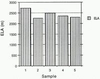
As expected, the mean surface area and the length are smallest for the simple valley glaciers in sample 1 (Fig. 1). At the same time, b up and b t are less positive and more negative, respectively, for sample 1 compared with the Other samples (Fig. 2). The elevations (Z up, Z t Z m) and the ELA are higher and E is larger in sample 1 than in other samples (Figs 3 and 4 and bottom lines in Table 1). For each of the samples, the next section explores correlations between the various glacier parameters.
Results
Within a given sample, two properties (such as terminus balance and length) were selected for each glacier. Both linear and power-law correlations were calculated between these two parameters. Similar linear and power-law correlations were determined for all other pairs of parameters commonly used in monitoring glaciers (i.e. the previously-mentioned S, x, Z up, Z m, Z t, ELA, E, b n, b t, and b up). Correlations were also performed between each of these parameters and potentially useful combinations of parameters, such as the total range in elevation (Z up, – Z t) and the range in mass balance (b up – b t). We emphasize that all of these correlations are spatial (between many glaciers) and not temporal; each glacier is assigned only one value for each parameter, for example an average ELA and an average net mass balance over the period of observation (Table 1). The correlations for each pair of parameters in each of the Eve samples are listed in Table 2.

Fig. 1. Histogram of surface area, S, and length, x (along center line), averaged by sample.

Fig. 2. Histograms of mass balance at the head of the glacier (bup), annual or net mass balance (bn) and mass balance at the tongue (bt), averaged by sample.
The glaciers in each sample are different in shape and type and reside in many different geographical regions. Thus, correlations between properties apply to all glaciers globally rather than to any individual glacier or mountain range. For example, for individual glaciers, a strong correlation between interannual variations in b n and the ELA is widely recognized (see, e.g., GMB, 1991, 1993, 1993, 1996). However, for all 80 glaciers considered simultaneously (using the temporal mean values of b n and ELA for each glacier), the correlation between b n and the ELA is almost non-existent (see Table 2).
For all live samples we have calculated about 130 correlation coefficients (r) for both linear and power-law regressions. In many cases the coefficients of correlation are very weak, but we report them for two reasons. First, our dataset is larger than any other previously analyzed, and it is useful to know that larger datasets do not improve the correlations found in previous analyses with smaller datasets. Second, in addition to recommending strong relationships, we can also note which correlations are not useful for global monitoring programs. Some of these poor correlations may seem obvious, bill many others are not. The most important of the possible correlations between combinations of parameters listed in Table 2 are noted here and discussed in the next section.
-
1. Net or annual specific mass balance (for simplicity we do not distinguish between these two balances). The correlation between b n and b t is weak, with r = 0.4 for simple valley glaciers and 0.44 for compound valley glaciers. Correlations between b n and E, ELA and all elevations (Z m, Z t, Z up) are also very weak. The correlation between b n and b up is poor for most samples, although significant (r = –0.72) for simple valley glaciers (sample 1). On the other hand, a good linear correlation (r = 0.6–0.8) occurs between (b n –b t) and other properties, such as length x and differences in elevation (Z m – Z t), (ELA – Z t) and (Z up – Z t).
-
2. Terminus balance. b t is well correlated with the length of glaciers, especially in sample 1 (r = 0.75). The correlation coefficient for b t, vs b up is 0.65 for simple valley glaciers (sample 1) but is very weak for all other samples, especially for relatively large compound glaciers (sample 2; r = 0.2). The correlation coefficients for b t vs (ELA – Z t) and (Z m – Z t) are large for all samples (r = 0.7–0.8).
-
3. Mass balance at the head of the glacier. b up correlates best with length x (r = 0.76). In general, b up correlates well (around 0.6) with all measures of elevation (Z m, (Z m – Z t) and (Z up – Z t)).
-
4. ELA. The ELA is best correlated with the mean elevation Z m (r = 0.99). The correlation between the ELA and Z t and Z up is also > 0.95 for all samples.
-
5. Surface area. S is strongly correlated with many parameters, especially the length x (r = 0.82–0.95 for all samples) and various mass balances such as b t, b up, (b up – b t), and (b n –b t) (with r around 0.8 for sample 1). S is somewhat correlated with elevations (e.g. (Z up – Z t) and (Z m – Z t)), and is more weakly correlated with the ELA and Z m (r ≈ 0.4). The correlation of S with the activity index E is very weak.
-
6. Length. x is well correlated with many parameters, particularly Z t and differences in elevation such as (Z up – Z t). This is expected since x is well correlated with the surface area, which is also well con-elated with many other parameters.
Table 1. Characteristics of glaciers used for correlations

Table 2. Correlation coefficients between glacier properties. In each column the linear correlation coefficients are given first and power-law correlations second


Fig. 3. Glacier minimum (Zt) average (Zm) and maximum (Zup) elevations, averaged by sample.

Fig. 4. Equilibrium-line altitude (ELA), averaged by sample.
Discussion
Based on experience, simple physical arguments and previous analyses, many of the strong correlations are expected. For example, the correlations between many morphological properties (such as upper and lower elevations, the range in elevation, length and surface area) have obvious physical explanations: the larger a glacier’s area the greater its length (Reference BahrBahr, 1997); and the higher Z up (the higher the mountains), the larger the size and length of glaciers. Nevertheless these strong correlations may be helpful for global monitoring because only one of the three parameters (area, length or elevation) is available in many cases.
A similarly reasonable and strong correlation between the ELA and the mean elevation has been suggested (personal communication from A. Ruddel, 1997). When averaged over long time-spans, the EEA is always close to Z m and will also have a strong correlation with Z t. Likewise, longer glaciers are expected to be strongly correlated with b up and b t, because the greater length implies a greater range in altitude and a greater span in climate conditions. An obvious reason for some of the weak correlations between the net mass balance and other parameters, such as elevation and area, is that b n ≈ 0 for all glaciers that are in or nearly in a steady state, regardless of the size of the glacier.
However, many of the correlations are not expected or do not have an immediate physical explanation. For example, the correlations between differences in mass balance (b up – b t, b n – b t, b n – b up) and any other properties are consistently better than the correlations between simple mass-balance measurements (b up, b t, b n) and these other properties. In fact, the good correlation between these differences in mass balance and glacier length, surface area and range in altitude (Z up – Z t) suggests that these parameters would be good for global glacier monitoring.
On the other hand, there is a very weak correlation between the ELA and glacier mass balance for all samples. On individual glaciers, the ELA is known to correlate very strongly with b n (GMB, 1991, 1993, 1994, 1996). However, the global spatial correlation between net mass balances is very poor (Reference DyurgerovDyurgerov, 1994; Reference Cogley, Adams, Ecclestone, Jung-Rothenhäusler and OmmanneyCogley and others, 1995) because glaciers occur in a wide variety of climatic zones from polar to temperate. We expect, therefore, that the ELA would also have a poor spatial correlation, and it is not too surprising that the correlation between the net mass balance and the ELA is poor.
Similar arguments suggest that the activity index, E, would be a poor tool for global glacier monitoring. Likewise, the very weak correlation between b n and b t for all samples prevents the net balance from being replaced by simpler measurements of the balance at the terminus. Measuring b t (and one or two stakes in the vicinity of the ELA) is not a good strategy for global mass-balance monitoring (Reference HaeberliHaeberli, 1995).
The simple valley glaciers (sample 1) frequently have stronger correlations than other samples. The reasons for this are unclear, although sample 1 is the most homogeneous in size and type. However, in several cases, the correlations in sample 5 (all glaciers) are at least as large as the correlations in other samples. This is true, in particular, for power-law correlations and for parameters that are common in routine glaciological work (e.g. surface area, length, ranges in elevation and ranges in mass balance such as b up – b n and b n – b t). The global properties of such parameters may be observed and studied without differentiation by groups or samples.
Conclusions and Recommendations
Net mass balance is typically used to monitor, understand and predict fluctuations in glacier volume, size and length. This relatively difficult-to-measure property (b n) might be replaced by other parameters (e.g. S, x, Z up, Z m, Z t, ELA, E, b t and b up), as long as the new parameters are well correlated with b n. Using a substantially larger dataset than in previous studies, we have calculated a large number of correlations to demonstrate which glacier properties might be useful as substitutes and which other properties would be less helpful (Table 2).
Most notably, correlations between net mass balance b n and the terminus balance b t are poor. Likewise the correlation between b n and b up is poor. Thus, despite previous suggestions, neither b t nor b up should be used as a replacement for b n in global monitoring strategies. On the other hand, the terminus balance is well correlated with (Z m – Z t). Because b t, Z m and Z t are easy to measure in the field and to derive from maps or remotely acquired images (in contrast to b n or the ELA), this relationship could be helpful in estimating the maximum ablation rate and total meltwater production over large regions. Ranges in mass balance (e.g. b up – b n, b n – b t and b up – b t) are also well correlated with many other parameters (e.g. ranges in elevation) and are usually better correlated than b up, b n or b t. Thus, the ranges in mass balance could be particularly useful in any of the global monitoring programs which have previously used only the direct measurements of mass balance (b up, b n or b t).
The correlations between the activity index and mass balances (b up, b n and b t) are weak. This implies that the activity index is a unique properly of individual glaciers and most likely reflects local and/or regional climate and topography, rather than global climate. Similarly, the correlations between ELAs and glacier mass balances (b up, b n and b t) are very weak. If necessary, though, the ELA may be replaced by Z m, Z t or Z up, as it is strongly correlated with each of these. This gives a nice technique for replacing a harder-to-measure climatically sensitive parameter with an easily measured altitude
Although, in many cases, the correlations between different glacier parameters are poor (Table 2), there are enough strong relationships to suggest that global mass-balance monitoring can be based on a relatively small subset of glacier properties. Some of these parameters (e.g. Z m, Z t, Z up, S, x) may be extracted from glacier inventories or determined from remotely sensed images (e.g. the difference between the ELA and Z m, Z t, Z up). Other properties (e.g. b t, b up, b n) have to be measured in the field on benchmark glaciers or calculated in models (e.g. Reference TangbornTangborn, 1980; Reference Oerlemans and PeltierOerlemans, 1993). The relationships (suggested by the strong correlations in Table 2) between these easy- and hard-to-measure parameters can help estimate glacier mass balances in entire mountain ranges or on a global scale.
Acknowledgements
We thank M. F. Meier, R. LeB. Hooke, and W. Tangborn for clarification of many points in the text. This study was supported by U.S. National Science Foundation grants OPP-9530782 and OPP-9634289.