


1. Introduction
The McMurdo Dry Valleys is one of the few ice-free regions in Antarctica. Consequently, it is one of the few places the glacially modified landscape can be used to infer past changes of the Antarctic ice sheet (Reference Denton and HallDenton and Hall, 2000). Large changes in ice-sheet extent, relative to the scale of the dry valleys, have been documented (Reference Hall, Denton and HendyHall and others, 2000; Reference Higgins, Denton and HendyHiggins and others, 2000). In contrast, the extent of the local alpine glaciers has changed little since the Pliocene (Reference Hall, Denton, Lux and BockheimHall and others, 1993; Reference Wilch, Lux, Denton and McIntoshWilch and others, 1993). Yet the small changes in the alpine glaciers are important to the maintenance of the enclosed ice-covered lakes in the dry valleys and, in turn, to the ecosystems that inhabit the valleys (Reference Fountain, Dana, Lewis, Vaughn, McKnight and PriscuFountain and others, 1999). We use repeat photography to quantify the change in extent of several glaciers over the past 20 years. To interpret these changes, we developed a numerical model to examine possible processes controlling the observed changes. Results from this study are important to several glaciological issues. First, the results bear on the possibility of using glacially modified terrain around these glaciers for paleoclimatic reconstruction. This is particularly apt in view of the climatic results obtained from the Taylor Dome ice core located about 100km away (Reference SteigSteig and others, 2000). Second, a history of glacier advance and retreat will help define the history of ice-dammed lake formation and drainage, a subject important to ecological evolution within the valleys (Reference Fountain, Dana, Lewis, Vaughn, McKnight and PriscuFountain and others, 1999). Third, we use our model to explore the response of polar alpine glaciers to climatic variations, a subject that has not been as thoroughly explored as for their temperate counterparts.
2. Site Description
The McMurdo Dry Valleys are located in southern Victoria Land on the edge of the Antarctic continent (Fig. 1). They are named the ‘dry valleys’ (Reference ScottScott, 1905) because the Trans-antarctic mountain range blocks the seaward expansion of the East Antarctic ice sheet (EAIS) and the valleys are largely empty of ice. A few outlet glaciers from the ice sheet terminate in the western ends of the valleys. Alpine glaciers populate the mountains, the largest of which reach the valley floor. Average annual air temperatures in the valleys vary between –30 and –178C, and summer air temperatures typically reach only a few degrees above freezing (Reference DoranDoran and others, 2002b). Consequently, the glaciers in the valleys are polar and are frozen to the substrate (Reference CuffeyCuffey and others, 2000). Melting is restricted to the glacier surface and to the 20 m high vertical cliffs which define the glacier margin in the ablation zone (Reference ChinnChinn, 1985; Reference Fountain, Dana, Lewis, Vaughn, McKnight and PriscuFountain and others, 1998). Streams originate at the glacier termini and flow for perhaps 10 weeks during the austral summer (Reference McKnight, Niyogi, Alger, Bomblies, Conovitz and TateMcKnight and others, 1999). Some of the streams discharge into perennially ice-covered lakes, which are present in every valley.
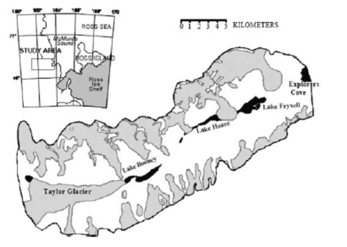
Fig. 1. Map of Taylor Valley, McMurdo Dry Valleys, Antarctica.
The annual mass exchange of these polar glaciers is relatively small compared to temperate glaciers. About 0.1m of snow accumulates in the upper zones and about 0.1–0.2m of ice is lost from the ablation zone (Reference Bull and CarneinBull and Carnein, 1970; Reference ChinnChinn, 1980; Fountain, unpublished data). Ablation in the accumulation zones is limited to sublimation and wind erosion. In the ablation zone, about 40–80% of the mass loss occurs through sublimation and the remainder is lost by melting (Reference Lewis, Fountain and DanaLewis and others, 1998).
The glacial history of the valleys is dominated by the activity of the EAIS. Taylor Glacier advanced almost to the eastern end of Taylor Valley about 70–100 kyr BP (Reference Hendy, Healy, Rayner, Shaw and WilsonHendy and others, 1979; Reference Higgins, Denton and HendyHiggins and others, 2000). During the Last Glacial Maximum, lowered sea levels caused the Ross Ice Shelf to advance. A lobe of the Ross Ice Shelf entered Taylor Valley about 23.8 kyr BP (Reference Hall, Denton and HendyHall and others, 2000) and blocked the seaward opening of Taylor Valley. A large ice-dammed lake formed, Lake Washburn, which persisted until about 6 kyr BP (Reference Hall and DentonHall and Denton, 1995). In contrast to these dramatic changes, geologic evidence indicates that the alpine glaciers of the valley have not significantly advanced from their present position since the Pliocene (Reference Hall, Denton, Lux and BockheimHall and others, 1993; Reference Wilch, Lux, Denton and McIntoshWilch and others, 1993). Reference Denton, Bockheim, Wilson and StuiverDenton and others (1989) suggested that the glaciers are currently in their most extended position within the past 12–14 kyr.
No long-term records of historic glacier change exist for the dry valleys. R.F. Scott’s expedition first visited Taylor Valley in 1903 (Reference ScottScott, 1905) and again in 1913 (Reference TaylorTaylor, 1916). Their photographs were used (Pe´we´ and Church, 1962) to assess changes in glacier extent. The results were inconclusive, partly because of the poor perspective of the photographs and partly because of the relatively small change in glacier extent. In the 1970s the New Zealand Antarctic Programme initiated a course of glaciological measurements in the valleys, which included photographs of the glacier termini (Reference Chinn and CummingChinn and Cumming, 1983). In anticipation of future photography, small cairns were erected at each camera location and identified by a metal stake. Some of these cairns were also used as a fixed reference to directly measure changes in glacier extent by using a steel tape to determine the distance to the glacier face. Reference ChinnChinn (1998) found that half the glaciers in valleys were advancing and the others were retreating. No measurements were made in Taylor Valley
Our study area is Taylor Valley, a 34 km long valley blocked in the west by Taylor Glacier, an outlet glacier from the EAIS (Fig. 1). To the east, the valley is open to McMurdo Sound. The Asgard Range, which rises to 2000 m, borders the valley to the north, and the Kukri Hills, rising to 1000 m, define the valley’s southern edge. The equilibrium-line altitude of the glaciers rises steeply to the west because of the sharp gradient in snow accumulation and sublimation (Reference FountainFountain and others, 1999).
3. Glacier Photography
3.1. Methods
During the austral summers of 1972/73 and 1977/78, three glaciers in Taylor Valley were photographed (Fig. 2) using a tripod-mounted camera with a 50 mm focal-length lens (Reference Chinn and CummingChinn and Cumming, 1983). The three glaciers are Canada Glacier, an alpine glacier 33.8 km2 in area; Suess Glacier, 12.2 km2 in area, which abuts against a large hill and spreads along the valley axis in two small lobes; and Taylor Glacier, an outlet glacier of the EAIS. We located the cairns established in the 1970s and, using the original photographs to capture the same scenes, we rephotographed (1995–97) the glaciers using a hand-held camera in a level position. The same-sized focal length lens (50 mm) was used as in the earlier photography. Small differences in vertical angle between the tripod and hand-held methods do not significantly affect the apparent glacier outline in the photographs. The fixed objects in the background (boulders, mountain peaks) of the photographs were used as reference points against which the position of the glacier outline was compared. We calculated the differences between the current and past glacier positions by measuring the true distances in the field and apparent distances from the photographs between the cairns, reference points and glaciers (see Appendix).
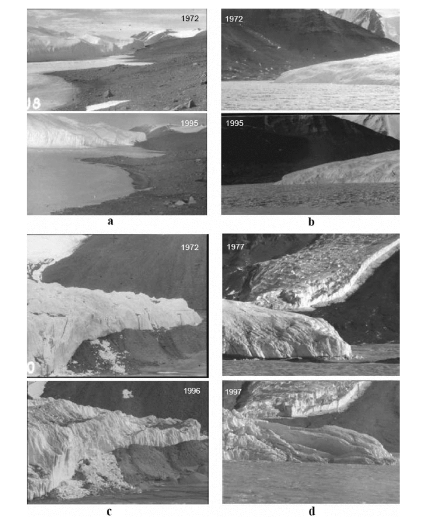
Fig. 2. Original photographs of glacier change: (a) Canada Glacier looking east, 1972–95; (b) Canada Glacier looking Reference DoranDoran and others, 2002b; north, 1972 –95; (c) Suess Glacier looking Doran and others, 2002bnorth, 1972–96; and (d) Taylor Glacier looking Reference DoranDoran and others, 2002b, north, 1977 –97. In (a) note the lake level rise with respect to the rocks in the foreground. In (d) the glacier in the background is Rhone Glacier.
3.2 Results and discussion
The approach seems to work well in that the estimated errors are substantially smaller, in most cases, than the magnitude of the change (Table 1). Two of the three glaciers measured advanced substantially. The change (advance) in Taylor Glacier is at least an order of magnitude greater than the observed changes of the other two glaciers. This might be expected because Taylor Glacier is an outlet glacier of the EAIS and is much larger than the alpine glaciers. In terms of fractional change in length relative to total length, the changes in Taylor and Canada Glaciers are quite similar, 0.11% and 0.17%, respectively.
Table 1. Changes in terminus position and glacier surface elevation determined from photographic analysis

Suess Glacier, on the other hand, is retreating. However, the retreat is probably due to local effects rather than a dynamic response of the glacier. Rock debris avalanches from the adjacent valley wall and mantles much of the east lobe of the glacier (Fig. 2c). The rock enhances ablation by reducing the albedo. In contrast, the west lobe of the glacier is free of rock debris, and its bulbous front with an ice cliff (not shown) seems to be advancing. A similar line of reasoning applies to Canada Glacier. The northwestern margin of the glacier (Fig. 2b) advanced 17m and coincides with relatively clean ice. The southwestern margin (Fig. 2a) is affected by debris and advanced about 2 m.
Note that all glaciers observed in Taylor Valley are thinning. This is expected for the retreating lobe of Suess Glacier, but it is unusual for advancing glaciers. If the geometry of a glacier front is thought of as a wedge, then as the glacier advances past a fixed point in space the surface elevation will increase at that point. The thinning is probably due to increasing air temperatures, causing increased melting, as inferred from lake-level rise and thinning lakeice covers (Wharton and others, 1992).
Changes in glacier length are slow compared to changes in surface energy balance due to the relatively long response time of glaciers to changes in ice mass (Jo´han-Doran and others, 2002bnesson and others, 1989). For Canada Glacier, given current climatic conditions, the dynamic response time is about 103 years. Thus, the glacier advance observed today is a response to conditions over the past 1000 years. Reference DoranDoran and others, 2002b; Reference Lyons, Tyler, Wharton, McKnight and VaughnLyons and others (1998) infer a drawdown 1200 years ago of the lakes in Taylor Valley. Conditions were colder then by about 38C, based on temperature reconstruction from measurements in boreholes drilled into the valley floor (personal communication from G. Reference DoranDoran and others, 2002b; Clow, 1998). Presumably, colder temperatures reduced meltwater production and inflow to the lakes, and lake levels dropped as the ice covers sublimated. Without meltwater inflow to the lakes, which compensates for the mass loss to sublimation, lake volume decreases. Air temperatures warmed following the drawdown, and increased melt from the glaciers refilled the lakes. Perhaps the current trend of increasing lake levels and warmer air temperatures is a continuation of this long-term trend.
If air temperatures increased and glacial melt increased, then we might expect a glacier recession rather than the glacier advances that we observe today. One possible explanation is that with warmer temperatures snowfall increased in the upper reaches of the glaciers, more than compensating for the ablation due to increased melt. Although that is a possibility, there is no evidence linking increased snowfall and warmer temperatures. Also, no evidence exists for an increase in snow accumulation, based on the Taylor Dome ice core, located about 100 km away (Reference SteigSteig and others, 2000). We hypothesize that the warming air temperatures caused the glacier advance by warming the ice and decreasing its viscosity (Reference WhillansWhillans, 1981). To test this hypothesis a numerical model was developed to determine whether the current glacial advance could occur under constant mass-balance conditions with a climatic warming starting ~1000years ago. We also test how large an increase in snow accumulation could explain the same result.
4. Ice-Flow Modeling
4.1. Model description
We use a finite-difference, time-dependent flowband model of a valley glacier similar to other glacier flow models (Reference BindschadlerBindschadler, 1982; Reference WaddingtonWaddington, 1982; Reference MacGregor, Anderson, Anderson and WaddingtonMacGregor and others, 2000). The model is defined in a coordinate system such that x is the direction of ice flow, y is transverse to ice flow, and z is vertical, positive upwards. S denotes the glacier surface elevation, B denotes the bed elevation, and H = S — B is the ice thickness. Ice flow in the downstream direction is calculated in a flowband of variable width W (x), which parameterizes converging or diverging flow in the y direction. The flowband is essentially bounded by two parallel streamlines across which mass does not flow. The incorporation of ay dimension allows the model to conserve mass within the body of the glacier and it exchanges mass at the surface through the surface mass balance. Glacier thickness changes are calculated by solving the mass continuity equation:
where Q is the ice flux and b is the surface specific mass balance. Ice flux is calculated as:
where us is the surface velocity on the center line, W H is the flowband cross-sectional area and f*(x) is the shape factor, the ratio of velocity averaged over W H to the surface velocity along the center line (Reference NyeNye, 1965). Surface ice velocity along the center line us is calculated assuming ice deformation follows a Glen-type flow law (Reference GlenGlen, 1958).
where n =3 is the flow exponent, ρ is the ice density, g is the gravitational acceleration, E is an enhancement factor and A is the temperature-independent softness parameter. We assume a no-slip basal boundary. Because drag along the valley walls supports some of the weight of the glacier, a shape factor, 0 < f < 1, is used to reduce the basal shear stress (Reference NyeNye, 1965; Reference BindschadlerBindschadler, 1982).
The typical expression for the softness parameter, A (T (z)) = A 0 exp (—Q/RT’(z)), is a function of temperature, where T is the ice temperature, Q is the activation energy for creep, and R is the gas constant (Reference PatersonPaterson, 1994). To simplify the calculations, we use a temperature-independent softness parameter A which generates the same surface velocity as the temperature-dependent softness parameter A(T(z)). To determine A, we calculate the temperature profile T(z) using a one-dimensional (vertical) steady-state temperature model (Reference Firestone, Waddington and CunninghamFirestone and others, 1990). In this advective-diffusive model of heat flow, the bed is assumed to be below the pressure-melting point, and the surface mass balance, surface temperature and geothermal heat flux are the boundary conditions. The resulting temperature profile, T(z), is used in a temperature-dependent Glen flow law to calculate the surface velocity us by integrating from the bedrock B to the surface S:
We equate the surface velocity using a temperature-dependent softness parameter (Equation (4)) to the surface velocity calculated using a temperature-independent softness parameter (Equation (3)) and solve for A~:

We recalculate the flow parameter A~ any time the ice thickness changes by >20 m, because ice-thickness changes cause changes in T (z) and corresponding changes in A~. The value of 20 m is chosen because we neglect the temperature changes in the upper 20m of the glacier due to the seasonal cycle (which we do not model), and focus on longer-term temperature changes which propagate deeper into the glacier and determine ice viscosity.
Historically, the shape factor, f*, has been applied to temperate (isothermal) glaciers and relates the measured surface velocity on the center line to the velocity averaged over the glacier cross-section (Reference NyeNye, 1965). Polar glaciers, like those in the dry valleys, have warmer (and consequently softer) ice near the bed than near the surface. Furthermore, since ice thickness varies along the cross-section, the basal temperature also varies. Thinner ice at the margins of a polar glacier is colder and stiffer relative to the basal ice in the center. Therefore, the shape factor as applied to polar glaciers incorporates two separate effects: channel shape and temperature. The model does not distinguish between these two effects.
4.2. Model application and results
We cannot apply the model to Canada, Suess or Taylor Glacier because of the lack of measurements that define glacier depth, surface speed or mass balance. Instead, we examine Commonwealth Glacier, the neighboring glacier to the east of Canada Glacier, where a set of fundamental measurements exists. Commonwealth and Canada Glaciers are similar in that they both flow from the Asgard Range to the floor of Taylor Valley where they form broad fans of ice. Commonwealth Glacier is larger (51.5 km2) than Canada Glacier (33.8 km2), but not much longer, 13km vs 11.5 km.
Commonwealth Glacier also appears to be advancing, based on the morphology of the cliffs and position against its moraine (Reference ChinnChinn, 1985). Therefore, Commonwealth Glacier seems a reasonable proxy for the behavior for Canada Glacier.
Our application of the ice-flow model uses measurements of Commonwealth Glacier acquired during the 1995-98 field seasons. Surface elevation S was measured by global positioning system (GPS) surveys; ice thickness H was measured by radio-echo sounding from which bed elevation B was calculated. These data, including mass balance (Fountain, unpublished data), were measured at 20 marker poles drilled into the glacier. Surface velocity was determined through repeat GPS surveying of the marker poles in 1995 and 1997. For the temperature model, we use a geothermal flux of 77 mWm–2 (personal communication from G. Reference DoranDoran and others, 2002b; Clow, 1998) and a single value for the surface temperature of the glacier, T surface = -188C. Generally, W(x) can be interpolated from the surface velocity field. Since there are relatively few surface velocity measurements on Commonwealth Glacier, we estimate W(x) based on surface topography, and vary W(x) to match the model predictions to measured velocity. We also use an enhancement factor E(x) in Equation (3) to help the model match observations. Grid spacing (in x) is variable and gradually decreases from 200m in the accumulation area to a minimum of 25 m at the terminus.
The initial geometry used in the model was based on our observations of glacier length, ice thickness, mass balance and flowband width based on the surface velocity field. The initial model used a constant mass-balance gradient with time. The model was run for 15 000 years at annual time-steps, and the glacier geometry evolved until an equilibrium length and ice-thickness profile was reached (about 5000 years). Predictions of modern glacier length, surface velocity and ice thickness did not simultaneously match observations in spite of our attempts to adjust the model. Using measured values of b(x) and an enhancement factor E (x) = 1, we were able to match the glacier length and ice-thickness profile by adjusting W(x), but calculated surface velocities in the ‘neck’ (Fig. 3) were a factor of 3 too small. To match the measurements of length, surface velocity and ice thickness, we needed to adjust E(x), W(x) and the gradient of mass balance. Ice in the accumulation area needed to be softer than calculated (E (x) > 1) and stiffer than calculated in the ablation zone (E (x)<1). The difference may be due to the insulating effect of snow. Model results of heat transfer show that basal ice under the accumulation area is about 1 8C warmer than when the insulating effect of snow is neglected. A 18C warming reduces the initial estimate of ice stiffness by about 50%, close to our reduction of 40% used to improve the model fit. The mass-balance gradient used was steeper than observed, with accumulation rate 40% higher than measured in the accumulation area, and 350% greater mass loss in the ablation area. Because our interest is the dynamic response time of the glacier (Reference NyeNye, 1963), we chose to match the observed pattern of u s (x), at the expense of the mass-balance values, the implications of which will be discussed later. The resulting model creates a modern Commonwealth Glacier about 75 m longer than observed (0.6% error), with a similar ice-thickness profile, and similar surface velocities along the center line (Fig. 3). We use this glacier in subsequent perturbation experiments.

Fig. 3. Comparison of model results and field measurements. The modeled glacier thickness (a) is greater in the ablation zone than the observations, but matches well in the accumulation zone. The velocity profile (b) predicts a localized region of higher velocity than the measurements suggest. Since the overall flow field is not known, it is possible that the measurements were not collected along the central flowline of the glacier. In this case, we expect the true velocities to be somewhat larger than our modeled velocities. The terminus initially retreats as the model reaches equilibrium (c), and then advances to a steady-state position after 4000 years. Our modeled glacier is 75m longer than the measured flowline.
4.3. Glacier response to temperature changes
To investigate the dynamic response to a change in air temperature alone, we apply a step change to the surface temperature while holding the mass balance constant. A time-dependent advective-diffusive model of heat flow (Reference PatankarPatankar, 1980) tracks temperature changes in the ice. The temperature profile of the glacier T(x, z) is recalculated every 25 years, and the flow parameter A(x, z) is updated accordingly. Results show that the terminus position of the glacier responds modestly to temperature perturbations of 1, 2 and 38C (warming and cooling). Over a 4000year time interval, the terminus advances by 50 m for a 38C warming, 25 m for a 28C warming and is stable for a 1 8C warming. It is possible that a finer grid resolution might capture more details of terminus movement, but we believe that finer grid spacing is not warranted, given the limitations of the model, and relatively sparse surface data. Figure 4 shows the changes in the softness parameter A, ice flux Q and ice thickness H at a point in the ‘neck’ of the glacier (x = 8800 m) as a result of a 28C warming. The softness parameter (Fig. 4a) changes exponentially, with a characteristic time τ of 2000years. As the ice warms and softens, ice flux Q (and ice velocity) initially increases and reaches a maximum after 750years (Fig. 4b). As a result of mass continuity (Equation (1)) ice thickness H decreases (Fig. 4c). Following the initial maximum in Q, both Q and H decrease exponentially, with similar characteristic times of 1800 years.
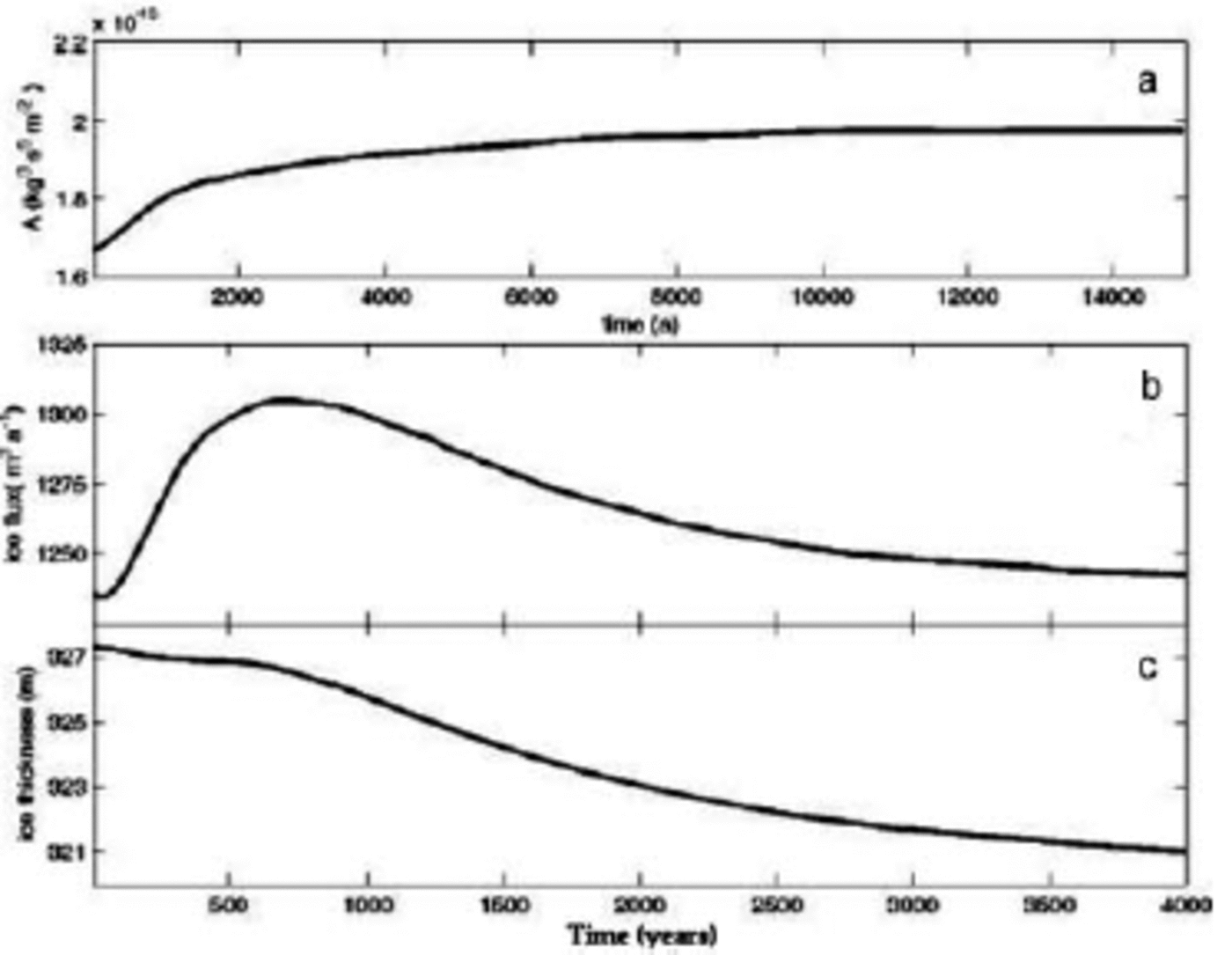
Fig. 4. Responses of softness parameter, ice flux and ice thickness at a point in the neck of the glacier (x = 8800 m) to a 28C warming at the glacier surface. The softness parameter (a) changes exponentially between the initial and final values as the warming penetrates the ice with a characteristic time-scale r of 2000 years. The changes of both the ice flux (b) and ice thickness (c) reach a maximum value after ~600years. Both ice flux and thickness approach final values asymptotically (τ ≈ 2000 years).
Glacier length does not change significantly after step decreases in surface temperature of up to 38C. Figure 5 shows the changes in A, Q and H due to a 28C cooling evaluated in the neck of the glacier (x = 8800 m) as in Figure 4. The softness parameter decreases exponentially with the same time constant (Fig. 5a) as in the warming case (r = 2000 years) and leads to a decrease in Q (Fig. 5b). Ice flux reaches a minimum about 750years after the step change in surface temperature. As a result of the reduction in Q, H (Fig. 5c) begins to increase after about 600 years. The gradual increase in H causes in a gradual increase in Q to pre-cooling levels after about 5000years due to the relationship between ice flux and ice thickness (Equation (2)).

Fig. 5. Responses of softness parameter, ice flux and ice thickness to a 28C cooling at the glacier surface. The softness parameter (a) changes exponentially between the initial and final values as the cooling penetrates the ice (τ = 2000 years). The ice flux (b) reaches a minimum after 750 years as a result of the decrease in softness. This reduction in ice flux leads to a gradual increase in thickness (c). As thickness increases, ice flux increases, reaching pre-cooling levels after 7000years. This balance between thickness and ice flux prevents any advance or retreat of the terminus in response to cooling.
4.4. Glacier response to mass-balance changes
To investigate the dynamic response to a change in mass balance, we apply a step change to the mass balance. We use a time-dependent advective-diffusive model of heat flow (Reference PatankarPatankar, 1980) to track temperature and viscosity changes resulting from ice-thickness changes, but we keep the surface temperature fixed at -180C.
We find that increasing the accumulation rate in the accumulation area by 7.5 mm a-1 (~10% increase over currently measured values) produces a 25 m advance, the same as predicted for a 28C warming. Ice thickness and ice flux reach new steady-state values after about 2000 years. In the neck of the glacier, the model predicts that the ice thickness will increase by about 3 m, somewhat less than the thickness increase caused by a 28C cooling. This time-scale is similar to the time required for kinematic wave propagation from the accumulation zone described by Reference NyeNye (1963). The time required for thermal equilibration is much longer than the kinematic time-scale. Consequently, the glacier geometry reaches a new steady state faster after an accumulation rate perturbation than after a thermal perturbation.
5. Discussion
The mismatch between the model results and the measured thickness, length, speed and mass-balance gradient on the glacier is curious. To explain the mismatch, we consider three contributing factors. First, shape factors were used to distribute the stress along the glacier cross-section (Reference NyeNye, 1965); these factors were developed for temperate (iso-thermal) glaciers. Polar glaciers are not isothermal, and have temperature gradients vertically through the ice column and horizontally along the bed. The stress distribution may be different in polar glaciers compared to isothermal glaciers as a result of non-uniform ice temperature, such that the shape factors should be revised for use in polar glaciers. We have relatively little information about the channel shape, ice-flow velocity or surface temperature at Commonwealth Glacier, so we do not attempt to revise the shape factors.
Second, the mass-balance gradient required to achieve a realistic glacier length is significantly larger than the measured gradient. The accumulation zone requires a 40% increase in net balance, and the ablation zone requires a 350% decrease. In absolute terms, the difference is not large, only 2.25 cm (from 5.50cm to 7.75 cm) and -25 cm (from -8cm to -31 cm), respectively. This result indicates that current mass-balance conditions may be insufficient to maintain the present length of the glacier. The required mass-balance gradient results in a greater ablation rate in the ablation zone and greater melting because the ablation due to sublimation weakly varies with temperature in comparison to melting (Reference Clow, McKay, Simmons and WhartonClow and others, 1988). The notion of a greater balance gradient in the past is partly supported by the observation that our measurements were made in the 1990s during a period of cooling air temperature, reduced meltwater runoff and dropping lake levels (Reference DoranDoran and others, 2002b; Reference DoranDoran and others, 2002a). This contrasts with previous decades of rising lake levels and the inferred rise since Scott’s expedition in 1903 and since modern observations began in the 1970s (Reference DoranDoran and others, 2002b; Reference Chinn, Green and FriedmannChinn, 1993).
Finally, there is uncertainty in both the flow velocity and depth of Commonwealth Glacier. A total of 20 point values of velocity and ice thickness at the mass-balance stakes does not provide the spatial density required to accurately resolve either glacier depth or flow speed. Given these limitations, the model results may not produce a numerically precise prediction of glacier change with temperature but will provide a reasonable representation of glacier behavior.
The model shows a 25 m advance for an increase in ice temperature of 2°C, at the limit of the model’s resolution. If there was a temperature increase about 1200years ago, according to Figure 4, ice flux in the ‘neck’ should have reached a maximum after ~750years, and should now be declining slowly. The ice viscosity should have achieved about half the total anticipated reduction by now as well. Based on this model, we expect another few meters of drawdown in the ‘neck’ and an associated gradual reduction in ice flux. This model also predicts thinning over the entire ablation zone. The ice thickness in the ablation zone initially increases, reaching a maximum after ~800years. The thickness increase is followed by a thinning of approximately 4 m over the next few thousand years.
Our model also predicts a 25 m advance for an accumulation rate increase of 7.5 mm in the accumulation area. If there was an accumulation rate increase 1200years ago, the ice flux and ice thickness in both the ‘neck’ and ablation area should still be increasing slowly. The model predicts a total ice-thickness increase of approximately 7 m in the ablation area, half of which is yet to come over the next 2500years. This result contrasts with the predictions of the warming-driven advance described above. Our photographic work suggests that the glacier termini are thinning, rather than thickening. This supports a temperature-driven advance rather than an accumulation rate-driven advance. Future measurements should be able to distinguish between these two possibilities.
Although the total predicted advance is small relative to changes in temperate glaciers and to changes in the outlet glaciers of the EAIS, this small advance can play a major role in the hydrology and ecology of Taylor Valley. If Canada Glacier retreats about 10m, Lake Hoare will flow into Lake Fryxell, thus eliminating one of the three major lakes in the valley. In addition to the disappearance of a lake ecosystem, a long stream channel, passing through the former lake basin, will be created. Water losses to evaporation and to the hyporheic zone (Reference Gooseff, McKnight, Runkel and VaughnGooseff and others, 2003) will alter the water, chemistry and nutrient fluxes to Lake Fryxell (Reference McKnight, Niyogi, Alger, Bomblies, Conovitz and TateMcKnight and others, 1999).
The flowband model illustrates the sluggish response of polar glaciers to relatively large changes in air temperature and supports similar results by Reference WhillansWhillans (1981). These results, perhaps, are expected from polar glaciers where the ice temperature is well below freezing and mass exchange is small. A 28C warming results in a 25 m advance of the glacier over a period of about 2000 years. In contrast, a 28C cooling does not result in a retreat, but rather a thickening of the glacier. These dynamic responses contrast with those of temperate glaciers. Also our work demonstrates that polar glaciers can readily advance but retreat slowly. Certainly, we ignore any possible effects of the change in air temperature on mass balance, but there is no clear linkage between the two for temperatures well below freezing. Only if the summer air temperature rises above freezing does ablation dramatically increase. Also, for glaciers that flow onto the relatively flat valley floors, changes in lateral extent are not accompanied by significant changes in elevation.
Previous work indicates that about 50% of the glaciers in the McMurdo Dry Valleys are advancing (Reference ChinnChinn, 1998). Most likely the differences can be explained by differences in glacier size (thickness). For example, smaller thinner glaciers in the valleys have a shorter response time and temperature-induced advance may have occurred some time in the past. Conversely, for very large glaciers, the advance might just be starting. A more complete answer to this question will require detailed study of both the small and large glaciers in the region.
6. Conclusions
Combining ground-based photography with field-based survey measurements allows us to calculate changes in glacier extent with known precision. In so doing we take advantage of archived photographs acquired decades ago to reveal slow changes inherent to the polar glaciers of the McMurdo Dry Valleys. While all glaciers are observed to be thinning, two of the three glaciers photographed have advanced. While these advances seem to indicate cooler conditions in this part of Antarctica compared to other areas of Antarctica (Reference DoranDoran and others, 2002b; Reference DoranDoran and others, 2002a) and contradict global trends of glacier shrinkage (Reference Dyurgerov and MeierDyurgerov and Meier, 2000), we propose that the advancing glaciers are caused by long-term climate warming.
We hypothesize that a reduction in ice viscosity, due to warmer temperatures, results in glacier expansion and thinning. To test this hypothesis we developed a flowband model of glacier movement, which incorporates a temperature-dependent softness parameter. Results show that an increase in air temperature eventually softens the ice as the temperature change is conducted through the glacier. Consequently, the glacier thins and advances about 25m for a 28C temperature increase. However, the response is not symmetric for a temperature decrease; the glacier remains in its extended position and thickens to a new equilibrium condition. This behavior is unique to polar glaciers. Furthermore, the modeling indicates that current glacier advance could be the result of a warming 1200 years ago, inferred from other studies (Reference Lyons, Tyler, Wharton, McKnight and VaughnLyons and others, 1998; G. Clow, unpublished information), with the maximum rate of advance peaking roughly 450 years ago. An accumulation rate increase could also be responsible for the advance. However, the model predicts glacier thickening as a result of an accumulation rate increase, in contrast to the thinning observed in the photography.
Perhaps equally intriguing is the difficulty in matching the model results with the observed values of mass balance, velocity, glacier extent and flow speed. Although the sparse dataset of field measurements and the formulation of the shape factor may contribute to the mismatch, different climatic conditions during the measurement period compared to previous decades to centuries cannot be excluded. Support for this notion is provided by the recent decline in air temperatures and lake levels during the measurement period in contrast to previous decades. Taken together, our findings indicate that the dynamic behavior of temperate glaciers in response to temperature changes cannot be directly applied to polar glaciers. The impressively sluggish behavior of polar glaciers is a consequence of the ice temperature and the small magnitude of mass exchange. These conditions mask an intriguing and complex response to temperature change that should be more thoroughly investigated.
Acknowledgements
Discussions with E. Waddington and H. Conway were valuable to our conception and treatment of this topic. P. Langevin took the photographs in the 1990s and made the enlargements. Reviews by J. Walder and K. Cuffey helped to clarify the manuscript. This work was supported by the US National Science Foundation (NSF) Office of Polar Programs (OPP 9211773 and OPP 0096250).
Appendix
To quantify the magnitude of glacier change, we needed to know the position of the fixed features in the background against which the terminus change is compared. For Taylor and Suess Glaciers and one view of Canada Glacier, the fixed features were boulders on the valley wall. In each scene, three boulders were identified on the image, and the distance and orientation from the camera location to each boulder was measured using a total station theodolite. For the eastern view of Canada Glacier (Fig. 2b), three peaks in the background were taken as the fixed points, the distance was estimated from a map, and orientation from the camera location was measured using the theodolite. For all images the distance to the glacier needs to be defined. An imaginary plane, parallel to the photographic (film) plane of the camera, was set equal to the distance from the camera focal point to the glacier horizon observed in the photograph. That distance was also measured by the total station. We assume that the distance does not change during the time intervals between photographs.
Each set of photograph pairs was enlarged to the same photographic scale, approximately equal in real terms to a 200 mm χ 250 mm print. To equalize the scale within each pair, the enlargement was adjusted so the apparent distance between the fixed features in the photos was the same. We assume that during the two-decade interval between photographs the ‘fixed’ features did not move. While this is certainly true for the mountain peaks, it is possible that the boulders may have moved. To account for this possibility, we compared the geometric relations between boulders on each image pair. In no case did any of the boulders change position during the interval between photographs.
To estimate vertical and horizontal changes in the glacier surface, the position of the fixed features was transformed from their true spatial position to their apparent position in the glacial plane as depicted within the image. The vertical angle to the fixed features is referenced to true horizontal. The angles in the horizontal plane (azimuth) were measured relative to an arbitrary origin (0°) set to the first feature measured. Because the reference angle from the plane of the film in the camera to the first feature was not measured in the field, it had to be determined from the field measurements and photographs. The measured azimuth angles between the fixed features and their apparent horizontal position within the photographic plane (parallel to the camera plane) were used in an iterative procedure to define the reference angle. From the reference angle and measured distances on the photograph, true horizontal distances were calculated using basic geometric relations for similar triangles and the true distances to each feature and to the glacial plane. Vertical elevations were then calculated based on the horizontal distances. The apparent heights of the fixed features above the glacier surface were then determined, and changes in glacier altitude between images were calculated. Numerous values of surface elevation change were calculated along the entire length of the glacier observed in the photograph. These values were averaged and presented as a single number in Table 1.
Photographs flatten perspective (depth of field), so one of the primary sources of error was the precise determination of the glacial plane in the field and the true distance to it. In the field we determined the range of possible distances to the plane. On the photograph the precision to which the distances between features could be measured was about 0.4 mm. Both of these known errors were included in the estimated error in the results. The unknown errors include uncertainty in the depiction of the glacial plane in the image and in possible distortions in the camera lens. We assume that the vector of glacier flow is parallel to the glacial plane, and we believe deviations from this are small. For changes in height of the ice surface, measurements on the photograph were made to the uppermost surface. However, it is clearly possible on a rough glacier surface such elements may be outside the glacier plane.


