


Background
Ice streams are responsible for discharging the majority of ice from ice sheets into the ocean (Rignot and others, Reference Rignot2008). As the ice approaches the ocean the speed of ice flow increases by 2–3 orders of magnitude relative to the ice-sheet interior and forms distinct bands of (~50–200 km) wide fast-flowing ice. Most modern and historically documented ice streams tend to be located in modest topographic depressions, form low-angle surfaces (e.g. < 1 × 10⁻³ grade) and are flanked and separated from slower moving ice by extensive shear deformation zones (Bentley, Reference Bentley1987).
Ice streams flow fast despite their relatively flat surface slopes due to slip at the ice–bed interface, which occurs by regelation or enhanced plastic creep (Cuffey and Paterson, Reference Cuffey and Paterson2010), or through pervasive deformation of the underlying till (Engelhardt and others, Reference Engelhardt, Humphrey, Kamb and Fahnestock1990; Kamb, Reference Kamb1991; Hermann and Barclay, Reference Hermann and Barclay1998; Tulaczyk and others, Reference Tulaczyk, Kamb and Engelhardt2000, Reference Tulaczyk, Scherer and Clark2001; Bindschadler and others, Reference Bindschadler, Bamber, Anandakrishnan, Alley and Bindschadler2001; Cuffey and Paterson, Reference Cuffey and Paterson2010; Zoet and Iverson, Reference Zoet and Iverson2018). The processes by which ice stream slip occurs are influenced by a complex interaction of factors including basal topography, subglacial drainage networks, water pressure, debris entrained in basal ice, substrate material properties, overburden pressure, driving stress and heat flow. The dynamic interaction of these factors on the small to medium scale gives rise to the macroscopic velocity field of all glaciers, and can result in transient phenomena such as kinematic waves (Weertman, Reference Weertman1962; Van de Wal and Oerlemans, Reference Van de Wal and Oerlemans1995), surging glaciers (Clarke, Reference Clarke1987; Sharp, Reference Sharp1988), drainage network reorganization (Nienow and others, Reference Nienow, Sharp and Willis1998), basal water pressure fluctuations (Stearns and others, Reference Stearns, Smith and Hamilton2008) and outburst floods (Walder and Costa, Reference Walder and Costa1996). Long-term macroscopic evolutionary trends, such as thinning and thickening of the ice, or the growth and stagnation of entire ice streams (Alley and others, Reference Alley, Anandakrishnan, Bentley and Lord1994), are on the whole driven by dynamic interaction of many small-scale components.
Though the beds of ice streams are difficult to access directly, geophysical methods find that ice stream beds are heterogeneous in strength and generally composed of deformable units of till (Blankenship and others, Reference Blankenship, Bentley, Rooney and Alley1986). Past observations have found that till thicknesses vary considerably beneath ice streams, and that bedrock highs may protrude through the till layer into the glacial sole (Muto and others, Reference Muto2019), affecting basal slip and basal seismicity (Zoet and others, Reference Zoet, Anandakrishnan, Alley, Nyblade and Wiens2012). Stronger portions of the bed which resist steady slip and produce elevated rates of basal seismicity are often referred to as ‘sticky spots’ (Alley, Reference Alley1993), and have been widely observed on many glaciers (Anandakrishnan and Bentley, Reference Anandakrishnan and Bentley1993; Stuart and others, Reference Stuart, Murray, Brisbourne, Styles and Toon2005; Smith, Reference Smith2006; Zoet and others, Reference Zoet, Anandakrishnan, Alley, Nyblade and Wiens2012; Allstadt and Malone, Reference Allstadt and Malone2014; Helmstetter and others, Reference Helmstetter, Nicolas, Comon and Gay2015; Smith and others, Reference Smith, Smith, White, Brisbourne and Pritchard2015; Barcheck and others, Reference Barcheck, Tulaczyk, Schwartz, Walter and Winberry2018). Sticky spots may occur at bed-rock highs protruding into the sole of the ice or at unusually competent till surrounded by more compliant till. Often, individual sticky spots have been identified as sources of repeating earthquake (or icequake) families, that may cluster in space or time and correlate with other observables such as basal water pressure, overburden pressure, solid Earth tides or temperature (Podolskiy and Walter, Reference Podolskiy and Walter2016).
Microseismic basal earthquakes (defined as dynamic slip events occurring faster than the steady-flow speed of the glacier) observed by seismic networks deployed on ice typically share several key characteristics: oftentimes waveforms are impulsive, of short-duration (e.g. < 0.5 s), have broadband frequency content (e.g. 5–250 Hz), and the magnitudes of sources are small (e.g. <M1). Waveforms of microseismic basal earthquakes are generally of short duration because the path effects that distort the source signal as it moves through the glacial ice are minimal. A possible source mechanism for basal earthquakes is the slip of debris-laden ice over bedrock highs protruding through the till (or large clasts embedded in the till) (Zoet and others, Reference Zoet, Anandakrishnan, Alley, Nyblade and Wiens2012; Lipovsky and others, Reference Lipovsky2019), though hydraulic fracturing (Zoet and others, Reference Zoet, Carpenter, Scuderi, Alley, Anandakrishnan, Marone and Jackson2013b), tensile failures (Walter and others, Reference Walter2009, Reference Walter, Dreger, Clinton, Deichmann and Funk2010), and shear events in the till have also been proposed as possible sources. Detection of these events automatically is often done by comparing a running short-term average to a long-term average (STA/LTA) of the seismic energy (Allen, Reference Allen1978), which becomes large when impulsive signals occur. Other commonly used techniques for detection are template matching (e.g. Allstadt and Malone, Reference Allstadt and Malone2014; Helmstetter and others, Reference Helmstetter, Nicolas, Comon and Gay2015) or visual inspection (e.g. Barcheck and others, Reference Barcheck, Tulaczyk, Schwartz, Walter and Winberry2018).
In contrast to observations of distinct stick-slip earthquakes, glaciers also produce sustained seismic tremors (MacAyeal and others, Reference MacAyeal, Okal, Aster and Bassis2008; Winberry and others, Reference Winberry, Anandakrishnan, Wiens and Alley2013; Lipovsky and Dunham, Reference Lipovsky and Dunham2016; Roeoesli and others, Reference Roeoesli, Walter, Ampuero and Kissling2016; Barcheck and others, Reference Barcheck, Tulaczyk, Schwartz, Walter and Winberry2018; Vore and others, Reference Vore, Bartholomaus, Winberry, Walter and Amundson2019). Seismic tremors are characterized by sustained, elevated seismic energy (e.g. minutes to days), harmonic resonances and overtones and emergent arrivals (Obara, Reference Obara2002; Shelly and others, Reference Shelly, Beroza, Ide and Nakamula2006). In the glacial setting, tremor originating from the bed has been linked to migrating fluids (Bartholomaus and others, Reference Bartholomaus2015; Vore and others, Reference Vore, Bartholomaus, Winberry, Walter and Amundson2019) and slow-slip earthquakes (Winberry and others, Reference Winberry, Anandakrishnan, Wiens and Alley2013; Lipovsky and Dunham, Reference Lipovsky and Dunham2017). Some types of basal tremors may represent rapidly repeating sequences of earthquakes, with a dominant resonant frequency equal to the average rate of distinct failures (Lipovsky and Dunham, Reference Lipovsky and Dunham2016). Generally, determining the precise source location of tremor can be difficult due to the lack of impulsive arrivals, though energy-based attenuation and beamforming methods have been used with some success (Larmat and others, Reference Larmat, Tromp, Liu and Montagner2008; Jones and others, Reference Jones, Kulessa, Doyle, Dow and Hubbard2013; Rösli and others, Reference Rösli, Walter, Husen, Andrews, Lüthi, Catania and Kissling2014).
In this study we report findings from passive seismic data recorded during a field campaign to the Greenland ice sheet (GIS) on the Northeast Greenland Ice Stream (NEGIS). The campaign occurred over several weeks during the summer of 2012 in central northeast Greenland and included the use of many geophysical analyses such as ground penetrating radar (Keisling and others, Reference Keisling2014), seismic reflection surveys (Christianson and others, Reference Christianson2014), shallow ice coring (Vallelonga and others, Reference Vallelonga2014), and geodetic monitoring (Riverman, Reference Riverman2017). In our analysis of the local seismicity we observe a range of seismic phenomena including: (a) basal microseismic earthquakes, (b) repeating earthquakes and the (c) occurrence of glacial tremor originating from the bed.
Setting
NEGIS extends 700 km into the interior of the GIS, nearly reaching the ice divide, and increases in velocity from 60 m a−1 at its initiation to >500 m a−1 at its terminus (Fig. 1), and drains ~11% of GIS land ice (Rignot and Mouginot, Reference Rignot and Mouginot2012). Basal topography mapped with GPR data indicate a relatively smooth, though non-uniform basal profile with ~200 m of bedrock relief between either side of the ice stream, and an average ice thickness of ~2700 m near its initiation zone (Vallelonga and others, Reference Vallelonga2014). Amplitude-vs-offset seismic analysis at NEGIS provided estimates that the bed was underlain by 7–12 m thick till with ~35% porosity. Outside the trunk of the ice stream, till with less porosity was inferred to be present (Christianson and others, Reference Christianson2014). In addition, Christianson and others (Reference Christianson2014) found evidence for dry (and hence strong) basal till directly beneath the southern shear margin of the ice stream. In agreement with this finding, Keisling and others (Reference Keisling2014) showed that the internal ice above the southern shear margin had highly deformed stratigraphy, which likely originated from anomalously high stress near the bed at the margin.

Fig. 1. Surface ice velocities of the GIS, and the spatial locations of seismometers used in this study. (a) Average surface ice velocities of GIS as measured by the Sentinel-1 satellite (Nagler and others, Reference Nagler, Rott, Hetzenecker, Wuite and Potin2015). Data are shown in polar stereographic projection with central meridian at 45° W and standard parallel at 70° N. To improve color contrast, ice velocities above 400 m yr−1 are displayed at a constant color value. (b) The local seismic array of six stations used in this study. Locations are shown in a local Cartesian frame, with the x and y axes aligned with geographic east and north, respectively. Approximate ice flow direction is shown by the blue arrow.
The existence of an ice stream penetrating deep into northeast Greenland has raised a number of questions, as it does not lie in a topographic depression along much of its length, and also does not show significant contrasts in bed material across the shear margins of the glacier (Fahnestock and others, Reference Fahnestock2001; Christianson and others, Reference Christianson2014). Elsewhere, these characteristics have largely been regarded as important for ice stream formation (Cuffey and Paterson, Reference Cuffey and Paterson2010). However, throughout central Greenland a pervasive geothermal heat anomaly is present (Fahnestock and others, Reference Fahnestock2001; Petrunin and others, Reference Petrunin2013; MacGregor and others, Reference MacGregor2016), perhaps resulting from crustal thinning caused by the passing of a hot spot beneath Greenland sometime during the late Cenozoic (Mordret, Reference Mordret2018; Rysgaard and others, Reference Rysgaard, Bendtsen, Mortensen and Sejr2018). Hence, there is a strong possibility that over geologic time the high geothermal heat flux induced basal melting and the subsequent development of fast ice flow.
Data
Seismic data were collected on six broadband seismometers in the interior of Greenland, centered at [75.62° N, 35.90° W]. The instruments were deployed from 15 June to 8 July 2012, with an average of 17.6 days of data collected from each (Table 1). The network was composed of four Nanometrics Trillium seismometers, with Taurus Digitizers sampling at 200 Hz, and two Nanometrics Trillium seismometers, with Reftek 130 Digitizers sampling at 250 Hz. Seismic stations were buried 1 m below the surface, leveled and aligned (to within 0.5° horizontal and 2° N–S). The aperture of the network was ~15 km, with average inter-station distances of ~8 km. The stations were spatially distributed on an irregular grid with the long axis pointing along the ice stream flow direction (Fig. 1). We label all stations (ST1, ST2, ST3, ST4, ST7 and ST8) with indices (1, 2, 3, 4, 5 and 6), respectively, in this paper.
Table 1. Summary of the discrete earthquake detections

Number of detections, event rates, number of repeating earthquake families and time range active of all stations.
All collected data were processed with an anti-aliasing lowpass filter and resampled to a common sampling rate of 200 Hz and bandpassed between 5 and 80 Hz. This band was chosen to suppress low-frequency microseism noise and teleseismic arrivals while highlighting local impulsive events that would occupy that frequency band. The data used in this study are available from the XW seismic network hosted on IRIS DMC, and are also archived at https://uwmadison.box.com/s/hvjlu5fo7rk038l7dk2y5oykq8cmljz7.
Methods
Several processing steps were used to detect and characterize local earthquakes and glacial tremor. For discrete events, we describe our approach for arrival picking, arrival characterization and repeating earthquake grouping (clustering). For the seismic tremor, we define a continuous statistical proxy to help identify its occurrence, as well as describe our approach for estimating tremor migration directions and speeds across the network. We also describe a method for reconstructing tremor as a superposition of many rapidly occurring discrete events, using an empirical Green's function approach. A summary of key notation used in the work is given in Table 2.
Table 2. Notation and definitions

Waveform arrival picking
Single-station features such as the STA/LTA metric are commonly used to detect impulsive arrivals in continuous seismograms (Allen, Reference Allen1978). However, a shortcoming of the standard STA/LTA approach is that it is sensitive to changing noise levels and generally requires adaptively varying the triggering threshold if the background energy levels are non-stationary, which is common in the glacial environment. In many cases kurtosis-based arrival picking methods appear more robust to statistical fluctuations in the noise level (e.g. Galiana-Merino and others, Reference Galiana-Merino, Rosa-Herranz and Parolai2008; Baillard and others, Reference Baillard, Crawford, Ballu, Hibert and Mangeney2013). Hence, we chose to use a kurtosis phase picker in our work, which was effective at detecting microseismic earthquakes and produced very few false arrival picks, even when energy levels changed dramatically during tremor sequences.
We define our picking algorithm as simply a moving, centered-window estimate of the empirical kurtosis, where at each time step the maximum kurtosis value between the horizontal components is measured. For each ith station we compute


where u ij(t) represents the ith station's jth component time-series, the shorthand u ij(t − w : t + w) represents the centered window around time t of half-width w, x i represents the ith entry of a vector x and $\bar {{\bi x}}$ is the mean of x. Components are ordered HHE, HHN and HHZ for j = 1, 2 and 3, respectively. We only consider horizontal components in our processing since the vertical channel shows higher noise levels than the horizontal components. The value 3 is subtracted from Eqn (1b) because a normally distributed vector has (unbiased) kurtosis exactly equal to 3, and by subtracting this value the resulting metric measures deviations from a standard normal distribution. Intuitively, when the kurtosis is large the distribution of the data is highly ‘tailed’, implying the presence of many outliers (DeCarlo, Reference DeCarlo1997); a short-duration impulsive arrival surrounded by noise is an example of such a case, however a sustained high energy tremor signal is not. An example detection from using Eqn (1a) is shown in Fig. 2, in which a short-duration impulsive signal (<0.2 s) causes a significant increase in the kurtosis.

Earthquake location with single stations
The large spatial separation of stations (on average ~8 km), low-magnitude sources and high anelastic attenuation of glacial ice (Peters and others, Reference Peters, Anandakrishnan, Alley and Voigt2012) resulted in a majority of events being detected on only one station at a time, and never more than two stations at a time. A single-station location approach based on waveform polarity and S–P lag times was followed (Magotra and others, Reference Magotra, Ahmed and Chael1989) to estimate locations for events with both discernible compressional (P-) and shear (S-) wave arrivals.
P-wave polarization direction
To implement the location method of Magotra and others (Reference Magotra, Ahmed and Chael1989), the maximum polarization direction of each P wave was used to estimate the propagation direction of the wavefront. This was achieved via eigenvector decomposition of the ground-motion data covariance matrix (following Vidale, Reference Vidale1986; Jurkevics, Reference Jurkevics1988). Specifically, for a three-component slice of data, X, of length n, where X ji represents the jth component and ith time step of X, the covariance matrix of X is given by

where xj represents the jth row of X, and 〈xi, xj〉 is the dot-product between xi and xj.
Because Eqn (2) is a symmetric positive semidefinite matrix it has three real, non-negative eigenvalues λ1 ≥ λ2 ≥ λ3 ≥ 0, with corresponding orthonormal eigenvectors v1, v2 and v3 that satisfy σ(X)vj = λjvj for j=1, 2 and 3. By construction, the eigenvector corresponding to the largest eigenvalue, v1, approximates the direction in 3-D Cartesian space in which the P wave, which vibrates longitudinally, is propagating. We constrain all v1 to point downward, by multiplying v1 by −1 when necessary (which occurs since the sign of the P-wave polarity can vary depending on the source). The incidence angle is estimated with respect to the glacial surface (we approximate the glacier surface as horizontal) for each vector as $\theta _{\rm inc} = \arccos \lpar {\bi v}_{1\comma 3}\rpar$ , where v1,3 is the third component of v1, and incidence angles of 0° and 90° represent wavefronts propagating perpendicularly and horizontally with respect the glacial surface, respectively.
Hypocentral estimation
Once P-wave propagation directions are estimated with eigenvector decomposition of Eqn (2), event hypocenters are estimated by combining the propagation direction with the inferred source–receiver radial distance. The estimated radial distance is computed from the S–P arrival time difference, t d. For a homogeneous velocity medium with P- and S-wave velocities V p and V s, respectively, the source-to-receiver radial distance Δ and source coordinate h are given by


where yi is the Cartesian location of the ith station and v1 is the first eigenvector of the P-wave data covariance matrix (Eqn (2)).
Equations (3a) and (3b) assume that the ice is homogeneous and isotropic. In reality, there are vertical velocity and density gradients due to firn compaction (Vallelonga and others, Reference Vallelonga2014). At NEGIS, there is a ~70 m thick firn layer in the uppermost portions of the glacier (Christianson and others, Reference Christianson2014; Riverman and others, Reference Riverman2019). To account for this we set V p as varying continuously from 1000 to 3840 m s−1 between 0 and 70 m, and model the continuously bending P-wave with standard finite difference ray tracing (Červenỳ and others, Reference Červenỳ, Molotkov, Molotkov and Pšenčík1977). This allows the trajectory of the P wave to bend away from normal as it goes deeper into the ice and refracts due to the changing velocity structure. The linearly increasing velocity profile we use to account for the firn layer is an approximation to the density structure found in Christianson and others (Reference Christianson2014); however, firn has a broad range of V p values over many glaciers (Podolskiy and Walter, Reference Podolskiy and Walter2016), and so without further information we select this as a simple first order representation of the increasing velocity profile. We also note that Eqn (3b) uses a simplification, in which free-surface corrections are ignored, however for rays within ~20° of normal incidence this approximation is sufficient (Neuberg and Pointer, Reference Neuberg and Pointer2000).
Lastly, the homogeneous velocity model of this region was somewhat unconstrained at the outset of this study. Christianson and others (Reference Christianson2014) measure an average homogeneous V p = 3840 m s−1 using data from active seismic surveys, but do not constrain V s with any additional observations. We follow Christianson and others (Reference Christianson2014) in setting V p = 3840 m s−1 and compute location estimates over a range of possible V s values to determine for which range of V s events locate near the bed. Given our assumptions, the V s value which localizes events near the bed the most is V s = 1990 m s−1. This V s value is very close to the 1930 m s−1 value that is obtained using V p = 3840 m s−1 and the nominal Poisson ratio of 0.33, and hence does appear to be a reasonable shear wave velocity value of glacial ice.
Clustering arrival waveforms into repeating event groups
Inspection of detected events revealed that many waveforms were nearly identical. In other studies, grouping arrivals into their respective families has been carried out using event templates in parallel with the detection of earthquakes using the template matching (or matched filter) method (Gibbons and Ringdal, Reference Gibbons and Ringdal2006; Allstadt and Malone, Reference Allstadt and Malone2014; Helmstetter and others, Reference Helmstetter, Nicolas, Comon and Gay2015). Without having templates a priori, however, these methods are not directly applicable and a more general approach was required. We used the graph-based Markov clustering algorithm (MCL) (Van Dongen, Reference Van Dongen2000), which is a tool from the wider community detection literature (Lancichinetti and Fortunato, Reference Lancichinetti and Fortunato2009), and which is able to identify non-overlapping group assignments for all events based on pairwise waveform similarity, and hence can be used to extract template waveforms and identify event families.
The MCL method identifies similar populations of events by treating all events as nodes on a mathematical graph and extracting information between the pairwise edge structure of the graph (or adjacency matrix) using an efficient method inspired by random walks on graphs. Between each two nodes in the graph the edge weight is defined as proportional to the maximum cross-correlation coefficient between the waveforms associated with both nodes. That is, the adjacency matrix is given by

where xi,1, and xi,2 denote the ith event's east and north waveform components, respectively, and ⭑ represents the cross-correlation operation. This matrix is calculated separately for each station, and encodes each similar event pair as a high value (maximum of 1), and all dissimilar events as low values (minimum of 0). The matrix (or graph) is additionally sparsified by truncating all entries in H below 0.5 to 0 to ensure that non-zero entries represent actual significant waveform similarities (rather than spurious non-zero correlations). Lastly, in Eqn (4), the column-wise scaling coefficients, c j, are chosen to ensure the sum over each column is equal to 1 (e.g. $\sum _i H_{ij} = 1$ for $\forall j$
 ). Because the sum over each column is 1, the matrix resembles a stochastic matrix, or in other words a matrix that can be interpreted as encoding discrete transition probabilities between all pairs of nodes, and hence which can be used to simulate random walks on the graph.
The theory behind the MCL method is that by simulating a particular type of oscillatory stochastic flow, which is carried out by iterating two simple matrix operations of ‘inflation’ (given by the pointwise power operation, Hr), and ‘expansion’ (given by matrix–matrix products, H × H), the stochastic flow quickly converges to a sparse, asymmetric matrix with several key properties. In particular, for each node in the resulting matrix there is one outgoing edge, which connects either to itself (i.e. a self-loop), or to a different node in the graph. The nodes with multiple incoming edges from other nodes in the graph are cluster centroids, and generally resemble the most quintessential element of the set of waveforms assigned to a given cluster. Similarly, all of the nodes assigned to a cluster relate to waveforms of high similarity to the other events in the cluster. The subset of nodes which only have self-loop assignments are typically unique or anomalous signals and hence do not appear to be coming from any repeating group.
After the construction of the adjacency matrix there is no other free parameters of the MCL method beyond the single parameter r, which is interpreted to control the granularity or ‘fineness’ of the resulting clusters, where increasing r is generally associated with increasing the number of independent clusters. Since r relates to the pointwise powering operation, Hr, it is usually taken to be small (e.g. within the range r ∈ (1, 10)) to avoid numerical instabilities. To automate the selection of r we scan over a range of r values between (1, 10) and calculate the graph modularity (Newman and Girvan, Reference Newman and Girvan2004), which is a metric that measures how well a clustering assignment naturally conforms to the adjacency matrix of the original graph. Typically, maximizing modularity reveals optimal cluster assignments of a graph (Newman and Girvan, Reference Newman and Girvan2004), however we find that the r value associated with maximum modularity (r max) has a tendency to create large clusters that combine several similar but distinct families into one. This likely occurs because waveform cross-correlation coefficients of short duration impulsive signals can often be high even for waveforms of different event families. Hence, we opt to set r as r max + 2, which by our inspection establishes a reasonable balance between revealing a realistic number of families and ensuring clusters do not group many obviously different families into one. The resulting modularity scores as a function of r are shown in Fig. S1, which highlight that the modularity scores obtain a distinct global maxima as r is varied over (1, 10), implying that this procedure for selecting r is stable.
A schematic example of how the clustering algorithm sorts waveforms into common groups from an initially unsorted set is shown in Fig. 3. Here, four earthquake families are present, and MCL reveals the underlying grouping from the initially unsorted pairwise cross-correlation matrix (Eqn (4)). Some strengths of the MCL algorithm are that it is computationally efficient, uses pairwise information between all detections simultaneously, and also automatically infers the number of cluster centroids directly from the data. Nevertheless, many other techniques exist in the field of community detection and may have also been applicable to this problem (for a review, see Lancichinetti and Fortunato, Reference Lancichinetti and Fortunato2009).

Fig. 3. Schematic example of the waveform clustering method. (a) A small number of initially unsorted waveforms in a dataset. The presence of repeating earthquakes is unknown, potentially present, or not present. (b) Upon clustering with MCL, the resulting edge structure of the new graph assigns each element to a template group (or no group). The new sets of waveforms, once grouped together show high inter-group similarity and low similarity between dissimilar groups. The median stack of the aligned waveforms from each family is taken, to represent the template waveform, as shown in red. For illustration purposes, values in matrices are displayed as binary, however in practice non-zero entries are taken from the continuous interval $[0.5\comma\; 1] \subset {\open R}$ .
.
Continuous tremor detection proxy
A defining characteristic of tremor is that energy levels remain elevated for a long duration (e.g. minutes, hours or days) (Obara, Reference Obara2002; Shelly and others, Reference Shelly, Beroza, Ide and Nakamula2006). As such, an effective proxy for the detection of tremor is to compute statistical measures of the continuous-waveform data distributions over moving time windows (Rouet-Leduc and others, Reference Rouet-Leduc, Hulbert and Johnson2019). If seismic energies are elevated for a sustained duration of time then the interquantile range of the data distribution will increase compared with quiescent intervals. We implement this method and compute the interquantile range of the data, over time t, using a variable window duration w. The metric is define by,

which records the maximum value between the interquantile estimates of both horizontal channels. Similar notation is used as in Eqn (1a), and q p(·) represents the pth quantile of its argument. We remark that the tremor detection proxy (Eqn (5)) is flexible, since short-term and long-term transients can be measured by simply changing w. This metric is not infallible, as impulsive events will also increase Ci′(t), however when the window size of Eqn (5) is much larger than the duration of the transient those contributions are largely suppressed.
Glacial tremor migration
An additional feature of the tremor is that it appears to show slowly migrating moveouts across the seismic network numerous times throughout the study. For example, the tremor proxy curves (Eqn (5)) have pronounced maxima, observed across all of the stations at differing lag times, which are sometimes quite large (e.g. ~300–1200 s). The typical migration speeds of these events are much slower than elastic wave velocities in glacial ice (e.g. ~10's of m s−1 rather than 1000's m s−1), and hence the simplest explanation is that the source of elastic energy is itself migrating across the network.
To parameterize and measure this phenomenon a simple beamforming method was employed to estimate the migration directions and speeds. The tremor source was assumed to migrate across the network as a horizontally oriented plane-wave with a fixed azimuth α and migration speed s. This parameterization is chosen as it is the simplest representation with only two free variables (α and s). Parameter estimates are obtained by minimizing the misfit of such a plane-wave with the observed relative arrival times, τ, of the migrating tremor record across the network, where τi is the ith stations relative arrival time of the tremor transient. Using least squares minimization, the solution is given by

where · is the dot-product, yi is the ith stations location and the relative observed and theoretical times are offset by the baseline station, i = 0 (or a different station, if station i = 0 does not have an observed tremor arrival for a given migration event). In a local Cartesian frame where x and y are parallel to the local east and north geographic directions, respectively, the migration direction is given by the vector [−sin(α), cos(α)], where the azimuth α is measured counter-clockwise from geographic north.
In the formulation of Eqn (6), the definition of tremor arrival time (τ) is not exact because the tremor waveforms are typically emergent in nature. Relative arrival times were estimated by visually identifying a characteristic time on the tremor proxy curves (Eqn (5)) that was easily correlated across the network; for example, the maximum amplitude or the onset of the transient was chosen. Observation values were only picked once, and we report source parameters calculated directly from these initial picks (to help minimize bias).
Waveform inversion of tremor
A common interpretation of some types of tectonic tremors is that quasi-continuous signals are emitted from rapidly occurring discrete failures at the source location (Obara, Reference Obara2002; Shelly and others, Reference Shelly, Beroza, Ide and Nakamula2006). When the discrete failures occur at a rate higher than the duration of a typical waveform recording (or support of the Green's function path effect), then the recordings represent an interference of many overlapping waveform arrivals that, if observed individually, would have been impulsive. In accordance, glacial tremor has also been suggested to result from a rapidly occurring set of discrete stick-slip failures at the bed (Winberry and others, Reference Winberry, Anandakrishnan, Wiens and Alley2013; Lipovsky and Dunham, Reference Lipovsky and Dunham2016).
In order to test this model at NEGIS we construct a direct optimization problem where an observed signal d is modeled as the convolution with a fixed Green's function g and an unknown source time function s, by the well-known elastic wave representation theorem (Aki and Richards, Reference Aki and Richards2002, Eqn (3.23)). This formulation is analogous to stacking a fixed template g at a series of (to be determined) time coordinates. The univariate optimization problem is then given by


and the multivariate formulation, with three independent components (i = 1, 2 and 3), by


where the * in Eqns (7) and (8) represents the convolution operation. The second terms in Eqns (7a) and (8b) are L1-norm penalties applied to s, weighted by the parameter λ, which is used to promote sparse source activations. Constraints (7b) and (8a) ensures that the source time function is non-negative.
Formulations (7–8) are equivalent to the point source representation of the elastic wave equation (Aki and Richards, Reference Aki and Richards2002, Eqn (3.23)), where the moment tensor is subsumed into the path effect term. This simplification is allowed so long as d is assumed to be produced (or can be approximated) by a single path effect, g, and that the moment tensor is constant for all of the source activations. We discuss this assumption more in the Results section, however note that for repeating earthquake groups this assumption is relatively safe. The source time function is forced to be non-negative in accordance with the assumption that all moment tensors are fixed, and also because empirically we expect more stable and sparse solutions for s when only positive copies of g are forced to stack to reconstruct d.
We minimize Eqn (7) using stochastic gradient descent (Kingma and Ba, Reference Kingma and Ba2014) implemented with automatic differentiation software (Paszke and others, Reference Paszke2017) to iteratively optimize an initial random guess, s0 ~ Uniform(0, 1), until it converges. We show with synthetic tests that when g is known (or approximately know) this type of inversion is typically stable for a range of λ values (Fig. S3) and accurate reconstructions can be obtained even when event rates are high (e.g. >10 events s−1) and randomly occurring in time. We also give insight into how to evaluate which path effect, g, from a collection of different path effects, {gi}, is most likely the source of a given tremor recording. In particular, using synthetic tests we show that when all templates are used to reconstruct a synthetic tremor interval the template used to generate the tremor is also recovered as the one with minimum reconstruction error (Fig. S4), indicating that relative reconstruction accuracy can be used to assess which templates are likely the source of a given tremor record.
Results
Earthquake detections
During the 28 days of the seismic deployment, the kurtosis-based arrival picking method (Eqn (1a)) detected 6187 impulsive arrivals across all stations of the network. Each station detected differing numbers of arrivals, ranging between 30 and 82 detections/day, with an average rate across the network of 58 events/day (Table 1). Detection rates were highly non-uniform in time, with a large proportion of the events being detected during apparent swarms of activity (Fig. S5). This behavior is highlighted in Figure S5, where the cumulative counts of event detections are plotted for each station. The dominant shape of these cumulative count functions was either flat (i.e. long intervals with few or no detections), or transiently steep (i.e. high event rates), producing the stairstep-like appearance of the functions. In Figure S5 it is apparent several hundred events cluster near times of station deployment, likely due to anthropogenic sources, however, this only occurs within ~2–3 h of when stations are deployed or recovered.
A large majority of all impulsive events were only detected on a single station, and typically only with a single dominant phase arrival. Figure 2 shows a typical example of the kurtosis-based detection of a small microseismic impulsive source; the waveform shown in Figure 2 is an S wave, and is recorded across all three components. We infer that the majority of detections were of S waves, since S waves are more energetic than P waves in the far field (Aki and Richards, Reference Aki and Richards2002, Eqn (4.92)), and are more likely to be detected when arrival amplitudes are near the noise level. It is possible some detections are of surface waves, however most of the visually identified surface waves we have seen have had slightly lower frequencies than the body waves and are more emergent, and are thus not preferentially detected by the kurtosis-based picking algorithm that we have tuned to detect impulsive events. The assertion that many of the waveforms detected are S waves is justified post hoc, in which we discover P waves preceding many S-wave arrivals after stacking waveforms across repeating earthquake families. Other features of the detected arrivals were that they had a broadband frequency content (5–85 Hz), and waveform durations were on average ~0.25 s or less (e.g. see Figs 2, 4–6).

Fig. 4. A summary of all 1681 earthquakes detected on station ST2. (a) The log of the Fourier transform of all normalized HHE traces. (b) The log of the Hilbert transform of all normalized HHE traces. In both panels (a, b) gray lines are plotted for each trace, red line is the median of the set and dashed black lines represent the 68% confidence intervals (±1 standard deviation) of the stack. The relatively broadband and short duration signals shown for ST2 are largely characteristic of the other stations as well.

Fig. 5. Example repeating earthquake families and the templates extracted from each. In each panel (a–f) gray traces show individual events and the red trace shows the template for each family, which is the median trace across the stack. The station name and number of events in each family are listed.

Fig. 6. Example earthquake templates that show both P and S waves. The S–P lag time and the station are listed for each template in panels (a–d).
By implementing the MCL clustering algorithm (Eqn (4)) to the pairwise matrix of waveform similarities (calculated for each station separately), 105 distinct event families were identified, with ~2/3 of all events assigned to a repeating earthquake group with at least five members or more. Each family had a variable number of events, ranging between 5 and 115 events. Each station detected a variable number of families, ranging between 5 and 37 (Table 1). Each event family often had its events clustered in time (Fig. S6). Over time, a template's activity was usually confined to discrete intervals, and could abruptly cease, begin, or pause activity for differing time intervals (Fig. S6). In some cases these transitions are correlated with the onset of tremor; e.g. tremor begins and detections of discrete events then cease.
Among individual repeating earthquake families, the pairwise cross-correlation values were typically very high (e.g. ~0.75–0.95). As an example, waveforms from six different event families are shown in Fig. 5, where the individual waveforms (gray) are all nearly identical as indicated by their common overlap, particularly on the HHE and HHN channels. The red line in Fig. 5 represents the median of the traces in the family, and is the ‘template’ of its corresponding family.
After templates from each family were extracted, a subset of templates displayed both P and S waves (Fig. 6), indicating the original detection was of an S wave, but that a discernible P wave was present after stacking across the repeating event waveforms of a family. Among all 105 templates, 43 (40%) families displayed identifiable P waves in addition to S waves once stacked, which was determined though visual inspection of all 105 template waveforms. We remark that occasionally, both P and S waves are also observed for individual events.
Using the S–P lag times, we observe that radial distances between sources and receivers are ~3450 ± 750 m (Fig. 7b), which is ~750 m greater than the average thickness of the ice. Many of the P-wave polarization's clustered just off of vertical incidence (Fig. 7c), between ~2° and 15°, indicating a predominantly vertically upward traveling wave as measured at the surface. Combining the two measurements of radial distance and incidence angle, and using the single station location technique (Eqns (3a), (3b)), P-wave templates are calculated as having an average depth of ~2700 m, which is the approximate ice thickness when V s = 1990 m s−1. Over a range of V s = 1990 ± 100 m s−1, average locations are shown to vary between ±280 m of the bed (Fig. S2).

Fig. 7. Probability density functions (PDFs) of template earthquake incident angles, source–receiver distances, and vertical distances from the glacial bed. The PDFs of (a,b,c) are calculated with kernel density estimation (Epanechnikov, Reference Epanechnikov1969), a non-parametric approach to estimating PDFs by replacing all data-points with Gaussians of widths (σ), as listed in each panel, and stacking.
For events with incidence angles >15°, we opt not to use the single station location technique (Eqns (3a), (3b)), as the angles are beyond the critical refraction angle for our assumed firn-glacial ice velocity model. This occurs for 19/43 (45%) of the identified P waves. These sources may be from the surface at radial distances near the ice thickness, however there is a geometric argument which generally prohibits this: events are only observed on single stations, and sources at ~3–4 km horizontal radius would often be equidistant between multiple sensors. Other possibilities may be that polarity estimates are noisy for these low-SNR signals, or that the phase types are misidentified. For these reasons, and as our focus is on seismicity from depth, we neglect to back-project P-wave templates with incidence angles >15°, and Fig. 7a reports depths for events with polarities of <15° incidence only.
Tremor results
Using the interquantile metric (Eqn (5)) to measure the energy level over moving windows (30 and 120 s), it was revealed that tremors occur of both long (minutes to hours) and short (e.g. <2 min) durations. We primarily focused our analysis on the long-duration tremor. Individual tremor records typically had a broadband spectrum between 5 and 80 Hz, and also displayed gliding spectral lines and harmonic resonances in some instances (e.g. Fig. 8). While the tremor shapes varied, in general the energy was emergent and rose gradually over time, culminating in a distinct energy peak prior to tapering back down to background levels.

Fig. 8. An example of discrete events transitioning into tremor, in both the (a) temporal, and (b) spectral domains. (c, d) are insets from windows in (a) and (b), respectively. After t = 54,730 s, the tremor signal is apparent, which is preceded by hundreds of discrete failures occurring at a rate of ~1.8 events s−1. In the spectral domain of panel (b), the tremor is characterized by a prominent harmonic resonance of ~35 Hz.
Through comparison of the tremor proxy curves (Eqn (5)) of different stations, it was observed that many long-duration tremor records showed migration patterns across the seismic network (e.g. Fig. 9a). In Figure 9a we show the 30 and 120 s tremor proxy records for a representative event migrating across all six stations of the network, arriving with delays ranging from 50 s to over 1000 s. Notably, these lag-times far exceed max allowable travel times of elastic waves within the network (~12 s for S-wave moveouts). In this example the modified beamforming method (Eqn (6)) indicated the best fitting migration direction was approximately perpendicular to the ice flow direction and directed toward the east (or southern shear margin) at a speed of ~12 m s−1 (Fig. 9b). The best fitting plane-wave resulted in an RMS-residual of ~80 s, which is ~7% the maximum observed lag-time between stations for this event. Figures 9d, e show the distribution of best-fitting angular azimuths and migration speeds for 10 additional events that were analyzed (Table 3). There is a strong tendency for migration directions to cluster at ~290° azimuth, speeds between 4 and 12 m s−1, and RMS-residuals <250 s.

Fig. 9. An example of tremor migration as a plane-wave and summary statistics over several events. (a) An observed tremor record propagating across the seismic network, plotted as the 90–10% interquantile range of the seismic data, computed over moving windows of 30 and 120 s (5). The maxima of each curve is marked by a red circle and approximates the relative arrival time of the signal. (b) The inferred best-fitting propagation azimuth (α) and speed (s) with respect to the network (Eqn (6)). (d and e) Summary statistics over angular and speed measurements, for all tremor events listen in Table 3.
Table 3. Tremor moveout data
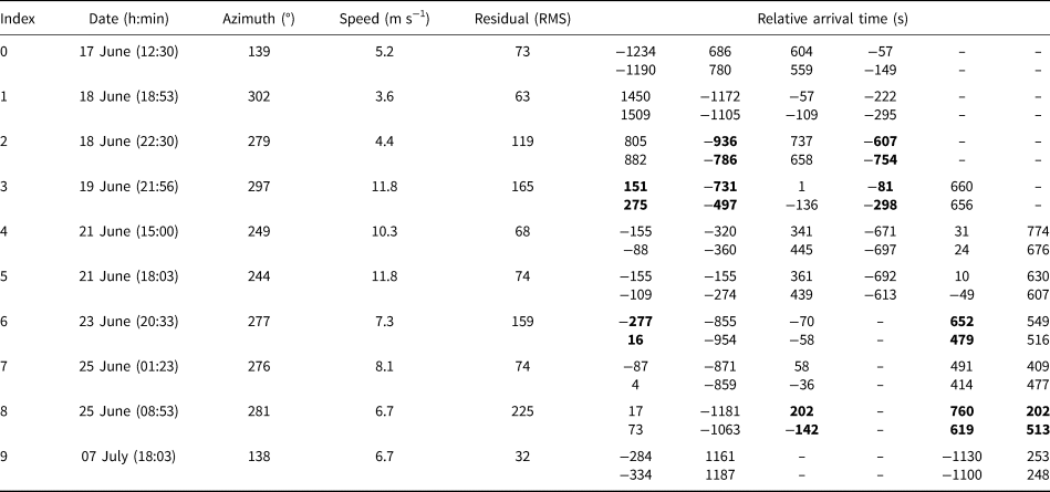
Observations of 10 well recorded tremor events that migrate across the network. (Left) Best fitting azimuths, migration speeds and minimum residuals. (Right) The observed (top) and predicted (bottom) relative arrival times for each event (and each station), obtained by minimizing the misfit of observed and modeled data (Eqn (6)). Residuals in the upper 20% percentile are highlighted in bold, and stations with no obvious arrival are left blank.
Another notable feature of the tremor was that occasionally a temporal relationship was observed between tremor and discrete failures. For example, in Fig. 8, many closely-spaced (in time) discrete failures occur in the ~100 s prior to the onset of short-duration tremor; the tremor signal is itself characterized by a spectral resonance at ~35 Hz. In another example, a set of repeating earthquakes (nearly all from a single event family) precede the onset of a long-duration tremor event for several hours (Fig. 10).

Fig. 10. Repeating earthquakes, glacial tremor and tremor inversion using several different path effects for the same tremor record. (a) Waveforms from 7 July 2012, of station ST2, HHN channel, showing a set of repeating earthquakes preceding the onset of tremor. Green circles denote discrete events all assigned to a single repeating earthquake group, and the tremor on the right-hand side contains the tremor signal used in the analysis of Fig. 11. (b) The reconstruction error of the tremor inversion results and cross-correlation coefficients of all 15 templates with the optimal template, which has minimum reconstruction error. The template with minimal reconstruction error (shown by a green circle) is the template associated with the set of repeating earthquakes shown in panel (a).

Fig. 11. An analysis of the tremor inversion shown in Fig. 10. (a) A 7 s tremor record from station ST2 (blue), with the inversion result (orange). (b) The spectrogram of the tremor shown in (a). (c) The source time function of the resulting solution, with individual peaks marked by green stars. (d) Moving window counts per second of discrete peaks of the source time function shown in (c). Window sizes increase from dark blue to light blue lines, ranging between 0.25 to 5 s windows. The ~26 Hz dominant resonance peak of the spectrogram shown in (b) is marked by a red line, which is nearly equal to the rate of discrete events occurring in time.
By representing tremor as the convolution of an (unknown) source time function with a known path effect it is possible to recover arbitrarily complex source time functions from the raw tremor signal (Fig. S3). The inverse problem (Eqn (7)) can be solved for even relatively complicated tremor signals, including those produced by the superposition of many rapidly occurring events (e.g. >10 events s−1). In applying the method to the representative tremor record shown in Fig. 10 we recover a relatively sparse source time function (we remark on the regularization term λ below); the solution vector is essentially represented by a collection of finite Dirac pulses (Fig. 11c). The average rate of source activations is found to be nearly ~26 Hz (Fig. 11d), which is equal to the dominant resonance frequency of the tremor, as shown by its spectrogram (Fig. 11b). For this example, a range of L1-norm penalty values for λ were tested; we used the λ from the ‘elbow’ of the resulting bias-variance trade off curve (Fig. S3).
In an additional test, we reconstruct a ~1.2 h slice of tremor (from the example of Fig. 10a), using station ST2 and all possible 15 templates associated with this station. Notably, we observe that the most optimal template for the reconstruction is the template associated with the sequence of repeating earthquakes that occurred in the hours preceding the onset of the tremor (Fig. 10b), and that all other templates have a reconstruction error that is negatively linearly related to the waveform similarity of each template with the optimal one. In other words, among all 15 templates – which are all active during different times of the studies duration – the best template for reconstructing the tremor is the one which produced the most recent repeating earthquake swarm. In addition, templates similar to the optimal one also reconstruct the tremor well and as templates increase in dissimilarity to the optimal template their reconstruction errors increase as well.
We justify our criterion for determining which template is the most optimal based on the following. First, the resulting solution of (Eqn (7)) has the least reconstruction error when using this template, compared against using all other templates (Fig. 10b). Second, we use synthetic tests to demonstrate that no matter which template (or Green's function) is used to construct a tremor signal (from the 15 possible templates), the reconstruction always has the minimum residual when the correct template is used in the inversion (Fig. S4). In addition, it is shown that the reconstruction error obtained for each template is (quasi-)linearly related to the waveform similarity between each template and the actual template used to produce the tremor. These findings show that relative reconstruction error among all templates is a valid diagnostic tool for determining which template is most likely the source of the tremor itself, at least when selecting from among several options.
Discussion
Observed signals
Two distinct types of seismicity were found abundantly at the NEGIS study site: discrete events and glacial tremor. The discrete events were characterized as broadband impulsive signals with short-durations (typically <0.25 s, Figs 2, 4–6), comparable to glacial microseismicity observed on numerous other glaciers around the world (e.g. Anandakrishnan and Bentley, Reference Anandakrishnan and Bentley1993; Smith, Reference Smith2006; Walter and others, Reference Walter, Deichmann and Funk2008; Allstadt and Malone, Reference Allstadt and Malone2014; Helmstetter and others, Reference Helmstetter, Nicolas, Comon and Gay2015; Barcheck and others, Reference Barcheck, Tulaczyk, Schwartz, Walter and Winberry2018). The kurtosis-based arrival picking method (Eqn (1a)) detected thousands of discrete events across the network, with an average rate of ~58 arrivals/station/day (Table 1). Several lines of evidence suggest many of the detected sources are localized near the glacial bed. These include: (a) the detection of S–P lag-times consistent with a source–receiver distance slightly greater than the local ice thickness (Fig. 7b), (b) the P-wave polarization indicating predominantly vertically oriented wavefronts (Fig. 7c) and (c) the backprojection of events close to the glacial bed (Fig. 7a). A subset of the P-wave polarities have incidence angles >15°, indicating polarities from sources that are potentially from near the surface of the glacier, or perhaps that have noisy polarity estimates or have misidentified phase types.
Many seismic swarms were also observed, as evidenced by transiently increased rates of detections lasting hours (Fig. S5). High cross-correlation coefficients between waveforms were used to identify that ~2/3 of all events originated from a repeating earthquake family. Within each event family, waveform shapes were nearly identical (e.g. see Figs 3 and 5), however the number of events that occurred in each family was variable. In addition, the events in each family tended to cluster in time, some event families abruptly ceased, and others were reactivated at different times throughout the study's duration (Fig. S6). Such evolution of event group activity may imply that the asperity contacts producing the discrete failures are gradually eroded or advected away (Zoet and others, Reference Zoet, Alley, Anandakrishnan and Christianson2013a), or that the local strain accumulation and its distribution across the glacial bed gradually shifts with time.
In parallel to the discrete event detections, glacial tremor was widely detected across the network and throughout the study duration. Frequently, tremor with durations of 100–1000's of seconds displayed an apparent moveout across the seismic network at speeds of 4–12 m s−1 toward the east (Fig. 9). The observed eastward migration direction is oriented obliquely across the ice stream's flow axis, migrating across the ice stream toward the southern shear margin. The slow migration velocity is far below elastic S-wave velocities of glacial ice, and is more consistent with a source of seismic energy migrating across the network. As the source migrates by, the local tremor signal is produced and observed only on the nearest stations.
The local tremor may be caused by mechanisms acting on the surface of the glacier, at the bed, or by processes unrelated to glacial slip. However, an apparent temporal relationship between discrete basal events and the tremor signals indicates a potential mechanistic link between the two types of seismicity. For example, in Fig. 8, a sequence of repeating basal events clusters in time, increasing in rate and moment release until a short-duration tremor signal is produced and the individual discrete events become indiscernible within the high energy signal. Another example is the earthquake swarm that preceded the onset of long-duration tremor as shown in Fig. 10.
In Antarctica, similar temporal relationships between discrete events and tremor have been observed on the Whillans Ice Plain (Winberry and others, Reference Winberry, Anandakrishnan, Wiens and Alley2013; Lipovsky and Dunham, Reference Lipovsky and Dunham2017; Barcheck and others, Reference Barcheck, Tulaczyk, Schwartz, Walter and Winberry2018). There, it was proposed that tremor was produced by rapidly occurring discrete failures at the bed (Winberry and others, Reference Winberry, Anandakrishnan, Wiens and Alley2013; Lipovsky and Dunham, Reference Lipovsky and Dunham2017). As the rate of stick-slip failures increases, the superposition of many discrete impulsive signals produces the characteristic tremor signal. We tested this model at NEGIS by constructing an explicit regularized inverse problem (Eqns (7–8)), where a tremor signal is represented as the convolution of a fixed path effect (Green's function) and an unknown source time function.
We obtain several noteworthy findings from applying this method to real data. For a representative tremor example (Fig. 10) the best fitting source function, which is composed of many Dirac pulses, has an average rate of source activations of ~26 events s−1, which is the same rate as the dominant resonance of the tremor itself (Fig. 11). This result is expected, since it was shown through numerical experiments that the rate of discrete failures should be equal to the dominant resonance of the tremor (Lipovsky and Dunham, Reference Lipovsky and Dunham2016). Additionally, when testing multiple possible path effects, the optimal path effect was from the repeating earthquake family that immediately preceded the onset of the tremor (Fig. 10). In other words, the data suggests a repeating earthquake swarm occurred in the same source region that shortly thereafter produced a long-duration tremor signal, that itself slowly migrates across the network.
We show through synthetic tests that it is straightforward to determine which path effect from a large collection of path effects is the most optimal for reconstructing a tremor sequence. In particular, we find that the correct path effect always has the minimum reconstruction error (Fig. S4). We also show that the relative reconstruction accuracy between all templates is primarily a function of the waveform cross-correlation similarity to the correct template (Fig. S4). Hence these synthetic tests help validate our inference that the template with minimum reconstruction error of Fig. 10b is the most optimal template.
Mechanical model
Combining our analyses of the discrete events and tremor we propose a conceptual model that links several of our observations together. We suggest that basal slip at NEGIS is accommodated primarily by stable-slip and deformation of a compliant velocity-strengthening till that is interspersed with a number of velocity-weakening sticky spots. The sticky spots serve as the origin for accumulated strain, which is released intermittently in the form of discrete stick-slip failures. The same asperities fail repeatedly, producing the repeating earthquake families, but over time (hours to days), stress is occasionally re-localized to different nearby asperities as contacts erode or are advected away. On an irregular time scale, an instability in the stress balance of the glacier occurs. This instability is driven by either ice strain imbalances (Zoet and others, Reference Zoet, Anandakrishnan, Alley, Nyblade and Wiens2012) or pore-water pressure transients (Iverson, Reference Iverson2010) that weaken basal till and promote an increase in the basal slip rate. The perturbation in basal slip rate propagates along the bed across the ice stream, generally to the east, resulting in the observed migration of the tremor signals (Fig. 9).
A possible mechanism driving this instability is unequal accumulation of pore-water pressures along the bed. Increasing pore-water pressures were proposed in the model of Lipovsky and Dunham (Reference Lipovsky and Dunham2016) as the primary driver of the transition to unstable sliding at WIP, and nearly the same mechanism has been invoked for migrating tectonic tremor observed at plate boundaries, including at the Cascadia and Mexico subduction zones (Cruz-Atienza and others, Reference Cruz-Atienza, Villafuerte and Bhat2018). Cruz-Atienza and others (Reference Cruz-Atienza, Villafuerte and Bhat2018) showed that tremor migrates across approximately dozens of km, often along the down-dip direction of the fault plane, at speeds on the order of 20–120 m s−1. The authors demonstrated with numerical experiments that over-pressurized fluids sourced from mantle dehydration reactions could induce localized slip by lowering the effective strength of the faults along the subduction interface.
The glacier regime may be similar to these tectonic settings, in which a complex drainage network at the bed is frequently re-worked, introducing small imbalances in localized fluid pressures at the bed. If stick-slip and pore-pressure variations are mechanically coupled to one another, feedbacks may allow discrete failures to locally increase the permeability and thereby increase the likelihood for additional instantaneous slip to occur. In particular, one possibility is that instantaneous slip induces the ice–bed interface to open along the lee side of asperities, causing the hydraulic permeability at the ice–bed to temporarily increase (Zoet and Iverson, Reference Zoet and Iverson2018). This lowers the effective stress of the contact and increases its likelihood for subsequent failure, and for the local expansion of the actively failing rupture front. This process may occur in a positive feedback loop, resulting in tremor being emitted from sticky spots across the bed as the rupture front migrates past them (Fig. 12). It is of note that the dominate tremor propagation direction to the east is approximately aimed along the contour of the inferred high pore-water pressure distribution at the study site (Christianson and others, Reference Christianson2014), highlighting the possibility that water pressure gradients closely interact with slip processes.

Fig. 12. A schematic example of the mechanical state we infer exists at the NEGIS study site. This displays the concept that there are two primary modes of behavior, slip and unstable slip. In stable slipping modes, weak compliant till allows continual slip, and periodically discrete stick-slip failures to occur on sticky spots. In this mode, discrete failures are largely uncorrelated, between stations, in time and space. In the unstable slipping mode, compliant till continues to undergo gradual slip, however sticky-spots begin to fail quasi-continuously. This mode is characterized by a source migration front, traveling across the network, that produces long duration seismic emissions (tremor) at each station as it passes by; the signals generally have few or no discernible impulsive arrivals, though are composed of many rapidly occurring and overlapping discrete arrivals.
An alternative, or perhaps simultaneous mechanism driving the transient tremor episodes, is that strain in the ice is unevenly distributed due to ice–bed interactions at the southern shear margin. Geophysical imaging of the southern shear margin ice shows highly deformed stratigraphy (Keisling and others, Reference Keisling2014), indicating that anomalously high strain occurs near the bed, which in turn is transferred into high differential strain of the ice. Christianson and others (Reference Christianson2014) found through a reflective seismic survey that the shear margins of NEGIS were anomalously stiff, and hence likely unsaturated. If the strong bed at the margins resisted the influx of ice into the central trunk of the ice stream unevenly, the tremor migration patterns toward the east (i.e. the southern shear margin) may be a mechanical response to equalize ice strain throughout the system.
In either case, transiently increasing pore-water pressures or differential strain localization toward the southern shear margin are viable candidates for creating an instability that is subsequently released in the form of a propagating slip transient that produces seismic tremor. Here we illustrate both phenomenon in the conceptual model of Fig. 12. We highlight both stable slip (non-tremor producing), and unstable slip (tremor producing) modes of NEGIS, with the possible mechanisms driving transitions between either state. In the future, a coupled hydrological and mechanical model may help reveal more insights into the dynamics occurring at NEGIS, and may help reveal which, if any, of these two hypotheses are most probable.
As the longest glacier of the GIS and one with large potential for sea level rise contribution, understanding the mechanics controlling the flow of ice throughout NEGIS is important for accurate modeling of the ice-sheet evolution. Our findings indicate that the bed of NEGIS is precariously balanced between stable and unstable slip, and that basal water pressures may play an important role in the local dynamics. As such, the ice stream may be sensitive to physical changes that affect the amount of available water. If surface melt increases in this region, as has recently been observed in the deep interior of GIS during anomalous warming events (Nghiem and others, Reference Nghiem2012; Hanna and others, Reference Hanna2014), liquid water could be funneled to the bed through crevasses found in the shear margins and perturb the mechanical state of the glacier. How such a perturbation would affect flow speeds and the widening or shrinking of NEGIS is an open question.
Conclusion
Physical processes inducing glacial seismicity typically involve mechanisms acting on time scales far shorter than what is captured by macroscopic observational tools such as GPS, InSAR, mass-balance analysis and geochemistry. Nonetheless, micro-mechanical processes dictate glacial deformation and slip and are therefore crucial to understand and quantify. Improved understanding of glacial micro-mechanical processes can help better inform glacier flow modeling and forecasts of glacial evolution in critical polar regions around the world. Studies of the GIS are of particular interest because GIS is experiencing rapid warming due to climate change, and comparatively less is known about the GIS as compared with the Antarctic ice sheet. In the long term, improved instrumentation of ice streams with seismic networks of small inter-station distances (e.g., ~1–3 km), and a survey spanning longer time intervals may enable more detailed insights into ice stream processes that are complementary to our findings. Additional analysis of time-dependent tremor features, such as possible correlations to tidal triggering (solid earth and ocean tides), or thermal drivers should be explored in greater detail.
Our work has shown that seismic data collected at NEGIS reveal two distinct phenomena: basal stick-slip events and glacial tremor. Both phenomena are observed to occur frequently throughout the summer of 2012, and we observe a strong link between the discrete events and tremor. We argue that discrete events show evidence for transitioning into a quasi-continuous slipping state, and that by increasing in rate the discrete event waveforms overlap in time to the extent they appear like tremor. The tremor is observed to propagate across the ice stream at speeds of 4–12 m s−1, indicating a transient increase in the basal slip rate or weakening of the basal till. This phenomenon is possibly driven by localized strain imbalances induced by stiff till at the southern shear margin or transient pore-water pressure fluctuations at the bed. These findings highlight the complex mechanical state that exists at NEGIS near its initiation zone and reveal the importance that basal water, and perhaps future ice surface melt, will play in the evolution of the glacier.
Supplementary material
The supplementary material for this article can be found at https://doi.org/10.1017/jog.2020.17.
Acknowledgments
Funding for this work was provided by CRESIS and the instruments deployed were loaned from PASSCAL. We would like to thank B. Lipovsky and one anonymous reviewer for helpful comments that improved the quality of this manuscript. We also thank field assistance from K. Christianson, D. Voight, K. Riverman and A. Muto. I. McBrearty thanks J. Woodard, D. Hanson, K. Feigl, C. Thurber and P. Johnson for helpful discussions and comments.


 Open access