


1. Introduction
Viscoelastic shear flows exhibit a range of chaotic dynamics depending on the flow parameters, from inertialess elastic turbulence (Groisman & Steinberg Reference Groisman and Steinberg2000) to a modified, drag-reduced, quasi-Newtonian turbulence when inertia dominates (White & Mungal Reference White and Mungal2008). Between these two extremes, a further chaotic flow state, elasto-inertial turbulence (EIT), can be sustained (Dubief, Terrapon & Soria Reference Dubief, Terrapon and Soria2013; Samanta et al. Reference Samanta, Dubief, Holzner, Schäfer, Morozov, Wagner and Hof2013). The area of the parameter space where EIT is found overlaps with various exact coherent states which connect to either Newtonian Tollmien–Schlichting (TS) waves (Lee & Zaki Reference Lee and Zaki2017; Shekar et al. Reference Shekar, McMullen, McKeon and Graham2020) or to a newly discovered centre-mode instability (Garg et al. Reference Garg, Chaudhary, Khalid, Shankar and Subramanian2018; Page, Dubief & Kerswell Reference Page, Dubief and Kerswell2020). This raises the intriguing question as to whether the self-sustaining mechanism of EIT is rooted in purely Newtonian or elastic dynamics, given recent evidence that the centre mode instability persists in the inertialess limit for extremely dilute solutions (Buza, Page & Kerswell Reference Buza, Page and Kerswell2021; Khalid, Shankar & Subramanian Reference Khalid, Shankar and Subramanian2021).
In planar flows, both elastic turbulence and EIT exist at subcritical parameter settings, which is in agreement with the known characteristics of the finite-amplitude travelling wave solutions which connect to TS waves and the centre mode (Page et al. Reference Page, Dubief and Kerswell2020; Shekar et al. Reference Shekar, McMullen, McKeon and Graham2020; Buza et al. Reference Buza, Page and Kerswell2021). Earlier work has also sought to connect elastic turbulence to linear instabilities in other configurations with streamline curvature in the basic state (e.g. Taylor–Couette flow Shaqfeh Reference Shaqfeh1996). In this scenario, elastic turbulence in parallel flows would always require a finite amplitude perturbation since these instabilities vanish in the absence of an elastic ‘hoop’ stress (Meulenbroek et al. Reference Meulenbroek, Storm, Morozov and van Saarloos2004; Morozov & Saarloos Reference Morozov and Saarloos2005). The need for a finite-amplitude perturbation is supported by experimental results (see e.g. Pan et al. Reference Pan, Morozov, Wagner and Arratia2013; Jha & Steinberg Reference Jha and Steinberg2020; Choueiri et al. Reference Choueiri, Lopez, Varshey, Sankar and Hof2021). In the original experiments by Pan et al. (Reference Pan, Morozov, Wagner and Arratia2013), a chaotic flow state was triggered with a sequence of cylindrical obstacles, though intriguingly at least  $n\geq 2$ cylinders were required. Inertialess viscoelastic flows also feature new linear transient growth mechanisms, the most significant being an inertialess version of ‘lift-up’ driven by polymer forces (Jovanovic & Kumar Reference Jovanovic and Kumar2010, Reference Jovanovic and Kumar2011). Given this subcritical picture, we focus here on a problem related to receptivity: how is streamline curvature in the bulk of a channel flow induced by surface roughness at the boundaries? We identify new mechanisms by which significant vorticity fluctuations can be established in the flow in both purely elastic and elasto-inertial regimes. Beyond the inherent interest in these flow patterns as a platform for secondary instability, we believe that the amplification mechanisms and associated asymptotic solutions will be of use in the study of the aforementioned instability waves, where the underlying mechanisms are unknown.
In earlier work (Page & Zaki Reference Page and Zaki2016) we studied the analogous problem in a Couette geometry, a viscoelastic version of the Newtonian analysis by Charru & Hinch (Reference Charru and Hinch2000). In viscoelastic Couette flow, the vortical response to a monochromatic boundary perturbation depends on the value of two dimensionless parameters:  $\alpha$, the dimensionless wavenumber of the surface distortions; and $\varSigma$, the ratio of a viscoelastic critical layer depth to the channel height. The viscoelastic critical-layer depth is the point at which the phase speed of (backward) propagating elasto-inertial waves matches the base-flow velocity. These elasto-inertial waves have a speed proportional to the square root of the streamwise normal elastic stress, analogous to Alfvén waves in magnetohydrodynamics (Chandrasekhar Reference Chandrasekhar1961). Across the layers in the flow where the base-flow speed matches the elastic wave speed the equations change type (a transition from sub- to supersonic, see Yoo & Joseph Reference Yoo and Joseph1985); at these points a resonance exists between the apparent frequency of oscillation of the wall to an observer moving with the base flow and the frequency associated with the elastic waves. This resonance results in a significant vorticity amplification in a thin region (Page & Zaki Reference Page and Zaki2016) driven by a kinematic reverse-Orr mechanism in the polymer torque (Page & Zaki Reference Page and Zaki2015), and the location of this layer delineates three regimes of vortical response in the Couette flow. (i) In shallow elastic flow, the channel depth is small compared with the roughness length scale, and the critical layer is outside of the flow domain; vortical perturbations fill the channel and the vorticity amplifies at the top wall. (ii) In elasto-inertial flows (referred to as ‘transcritical’ in Page & Zaki Reference Page and Zaki2016), the elastic critical layer is inside the flow domain and within a wavelength of the lower wall, leading to large vorticity amplification at that location via the resonance mechanism. (iii) In deep elastic flows the critical layer is far from the lower wall and the vorticity perturbation decays monotonically with height.
The three flow regimes were subsequently confirmed in experiments with real polymer solutions (Haward et al. Reference Haward, Shen, Page and Zaki2017, Reference Haward, Page, Zaki and Shen2018a,Reference Haward, Page, Zaki and Shenb) in a pressure-driven channel flow. In deeper channels (where the wall disturbance wavelength is much smaller than the channel depth), there is a near-exact correspondence with the Couette case, because on the length scale of the roughness the base flow looks like simple shear. However, in shallow channels, notably where experimental data are challenging to obtain, this will no longer be the case because the perturbation will feel the effect of the non-monotonic background velocity profile at leading order, even in the absence of inertia (where the Newtonian response would be insensitive to background velocity profile). These deviations are driven largely by the base streamwise normal polymer stress which is proportional to the local shear rate and, hence, vanishes at the centreline. This base-flow stress provides a mechanism for elasto-inertial wave propagation in flows with inertia and leads to a purely elastic response otherwise. Therefore, in shallow channels we must account for the fact that (i) there will be two critical layers in the flow domain where the base velocity matches the elastic wave speed and (ii) the vanishing elastic stresses at the centreline may disrupt the dominant balance that leads to vorticity amplification in the shallow elastic Couette flow. In this paper, we examine both of these effects in detail, where we show that both provide new mechanisms for significant vorticity amplification in shallow channels.
The remainder of this paper is structured as follows. In § 2, we introduce the governing equations and show numerically the new regimes in the flow over a long Gaussian bump. In § 3, we derive matched asymptotic expansions for the two new behaviours which appear in a viscoelastic channel under the joint assumption of long-wave disturbances and high Weissenberg numbers; we also discuss the amplification mechanisms. Finally, conclusions are provided in § 4.
2. Vortical response to wall roughness in viscoelastic channel flows
2.1. Set-up
We consider the pressure-driven, steady flow of an Oldroyd-B fluid in a two-dimensional, planar channel. The governing equations are
 \begin{gather} \boldsymbol{\nabla} \boldsymbol{\cdot} \boldsymbol u = 0, \end{gather}
 \begin{gather}\boldsymbol u \boldsymbol{\cdot} \boldsymbol{\nabla} \boldsymbol u ={-}\boldsymbol{\nabla} p + \frac{\beta}{R}\nabla^2\boldsymbol u + \frac{(1-\beta)}{R}\boldsymbol{\nabla} \boldsymbol{\cdot} \boldsymbol T, \end{gather}
 \begin{gather}\boldsymbol u \boldsymbol{\cdot} \boldsymbol{\nabla} \boldsymbol C + \boldsymbol T = \boldsymbol C \boldsymbol{\cdot} \boldsymbol{\nabla} \boldsymbol u + (\boldsymbol{\nabla} \boldsymbol u)^\top \boldsymbol{\cdot} \boldsymbol C, \end{gather}
where  $\boldsymbol T = W^{-1}(\boldsymbol C - \boldsymbol I)$ relates the polymeric stress and conformation tensor. The equations have been non-dimensionalised by the wall shear rate, $\dot {\gamma }$, and channel half-height, $d$, which defines the Reynolds and Weissenberg numbers as $R:=\dot {\gamma } d^2/\nu$ and $W:=\dot {\gamma }\varsigma$, respectively, where $\varsigma$ is the relaxation time of the polymer chains and $\nu$ is the total kinematic viscosity of the fluid; the parameter $\beta := \nu _s/\nu$ is the ratio of solvent-to-total viscosity.
In the absence of fluctuations, the streamwise-independent solution of (2.1) is the standard Poiseuille velocity profile with associated polymeric stresses
 \begin{equation} U(z) = \frac{1}{2}(1-z^2), \quad T_{11}(z) = 2W(U')^2 = 2Wz^2, \quad T_{13}(z) = U' ={-}z, \end{equation}
where  $z\in [-1,1]$ is the vertical coordinate, and primes denote derivatives of base-state variables. The linear scaling of the streamwise normal stress, $T_{11}$, with $W$ is the leading cause of deviations from a standard ‘Newtonian’ response, both in the channel configuration considered here and in the simpler Couette configuration (Page & Zaki Reference Page and Zaki2016).
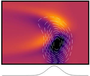
We are interested in the steady perturbation field induced by the addition of a small-amplitude surface roughness to the lower wall of the channel,  $z=-1+\epsilon h(x)$, where $\epsilon \ll 1$. A schematic of the configuration is shown in figure 1. Non-trivial vortical perturbations arise at $O(\epsilon )$ via a slip condition on the perturbation velocity at the lower wall, $u(x,z=-1) = -h(x)$ (in dimensional variables, $u^*(x^*,z^* = -d) = -\dot {\gamma } h^*(x)$), which results from the requirement that the total velocity vanishes on the solid boundary. The no-penetration condition, $w(x,z=-1)=0$, is unchanged in the linearised problem. Assuming it is suitably well behaved, we write our surface-roughness function as a Fourier series:
 \begin{equation} h(x) = \sum_\alpha \hat{h}_{\alpha} {\rm e}^{\mathrm{i} \alpha x}, \end{equation}
and solve for the monochromatic linear response to each individual surface wavenumber  $\alpha$,
 \begin{gather} \mathrm{i} \alpha \hat{u} + D\hat{w} = 0, \end{gather}
 \begin{gather}\mathrm{i} \alpha U\hat{u} + \hat{w}U' ={-}\mathrm{i} \alpha \hat{p} + \frac{\beta}{R}\left(D^2 - \alpha^2\right)\hat{u} + \frac{(1-\beta)}{R}\left(\mathrm{i} \alpha \hat{\tau}_{11} +D\hat{\tau}_{13}\right), \end{gather}
 \begin{gather}\mathrm{i} \alpha U\hat{w} ={-}D\hat{p} + \frac{\beta}{R}\left(D^2 - \alpha^2\right)\hat{w} + \frac{(1-\beta)}{R}\left(\mathrm{i} \alpha \hat{\tau}_{13} +D\hat{\tau}_{33}\right), \end{gather}
 \begin{gather}\mathrm{i} \alpha U\hat{\tau}_{11}+\hat{w}T_{11}' + \frac{1}{W}\hat{\tau}_{11} = 2\mathrm{i} \alpha T_{11}\hat{u} + 2T_{13}D\hat{u} + 2U'\hat{\tau}_{13} +\frac{2\mathrm{i} \alpha}{W}\hat{u}, \end{gather}
 \begin{gather}\mathrm{i} \alpha U\hat{\tau}_{13}+\hat{w}T_{13}' + \frac{1}{W}\hat{\tau}_{13} = \mathrm{i} \alpha T_{11}\hat{w} + U'\hat{\tau}_{33} +\frac{1}{W}\left(\mathrm{i} \alpha \hat{w} + D\hat{u}\right), \end{gather}
 \begin{gather}\mathrm{i} \alpha U\hat{\tau}_{33} + \frac{1}{W}\hat{\tau}_{33} = 2\mathrm{i} \alpha T_{13}\hat{w} +\frac{2}{W}D\hat{u}, \end{gather}
where the slip condition on the full velocity is scaled appropriately for each component wave,  $\hat {u}(z=-1) = -\hat {h}_{\alpha }$, and $D$ is the wall-normal derivative.

Figure 1. Schematic of the flow configuration considered in this paper, with variables shown in their dimensional form. The problem is non-dimensionalised by the channel half-height,  $d$, and the wall shear rate, $\dot {\gamma }$, of the base-flow velocity. A monochromatic surface topography is shown for illustration.
We are interested in both the response to localised roughness, which we explore numerically, and the vortical perturbations induced by monochromatic surface waves, which we examine with matched asymptotic expansions. For the numerics, we solve (2.4), and other similar systems appearing in this paper, using an expansion in Chebyshev polynomials in  $z$. Typically $N_c\approx 200$ polynomials is sufficient. The localised bumps considered in the following, for which (2.3) approximates a Fourier integral, require very long domains due to a significant long-wave response. In the calculations we set $L^*/l_x^*=400$ (where $L^*$ and $l_x^*$ are the dimensional computation domain and bump lengths, respectively) which defines the lowest wavenumber $\alpha _1 = 2{\rm \pi} l^*_x/L^*$. A total of $N_x=1024$ Fourier modes are used to construct the response.
2.2. Response to local roughness
In the Couette configuration studied by Page & Zaki (Reference Page and Zaki2016), significant vorticity amplification at high- $W$ occurred either at the top wall or at a critical layer in the bulk of the flow (where the base-flow speed is equal to the elastic wave speed; see discussion in § 1). New mechanisms for vorticity amplification are possible in the channel flow studied here, and will be shown to be associated with the non-monotonic base-flow velocity profile and the variation of the normal stress $T_{11}$ with depth $z$. Intuitively, these differences only manifest in shallow channels, where the characteristic length scale of the roughness, $l_x^*$, is comparable to or longer than the channel half-height, $d$. Small-scale roughness sees a background flow that locally is a close approximation to simple shear, and the corresponding Couette behaviour is recovered for the vorticity field.
The new regimes of vorticity amplification in a viscoelastic channel flow are summarised in figure 2, where the spanwise vorticity perturbations induced by a long Gaussian bump,  $h(x)=\exp (-x^2 / l_x^2)$, where $l_x:=l_x^*/d=2$, are examined for a particular set of viscoelastic parameters and three Reynolds numbers, $R\in \{1, 200, 2000\}$, alongside the response in a Newtonian fluid.

Figure 2. Response to Gaussian bump with  $l_x=2$ in (a,c,e) Newtonian and (b,d,f) viscoelastic flows with $W=200$ and $\beta =0.5$. The Reynolds number is matched between the Newtonian and viscoelastic calculations and increases from top to bottom, $R=\{1, 200, 1000\}$. Colours show the spanwise vorticity perturbation, lines are the perturbation streamfunction (solid black positive, dashed white negative).
For all three values of  $R$ in the Newtonian fluid, the response is a straightforward modification of the response in Couette flow to a channel geometry. At low- $R$, the perturbation field is a Stokes flow solution and is independent of the details of the background flow due to the absence of advection, a response which is identical to ‘shallow viscous’ flow in a simple shear (Charru & Hinch Reference Charru and Hinch2000). At higher Reynolds numbers, a shallow-channel version of the ‘inviscid’ regime of Charru & Hinch (Reference Charru and Hinch2000) is found, where the vorticity response at the lower wall is confined to a thin layer of thickness $\delta \sim R^{-1/3}$. There is a larger, irrotational flow response which fills the domain, and a weak vorticity perturbation is established in a thin wall layer around $z=1$ by adjustment to the no-slip boundary condition.
In contrast, the viscoelastic flow response is strikingly different to both the Newtonian flow fields and the response in a viscoelastic Couette flow at the same parameter settings for all three values of  $R$. In the near-inertialess flow at $R=1$, the vorticity is amplified around the channel centreline directly above the bump, with the elongated stripes of vorticity extending significantly upstream of the bump. This shallow elastic behaviour is markedly different from the same regime in Couette flow, where vorticity amplification occurs at the top wall.
At the largest value of  $R$, the perturbation vorticity is amplified in stripes which sit some distance from the lower wall. This shallow elasto-inertial response is familiar from the Couette configuration, where vorticity is amplified in a viscoelastic critical layer at which the base-flow velocity matches the elastic wave speed. In contrast to that behaviour, vorticity perturbations of a similar magnitude are also established on the opposite, smooth-walled side of the channel, presumably at a second critical layer. Therefore, although the penetration depth of the vorticity in an elasto-inertial Couette flow is proportional to the critical layer depth, here the vortical perturbations fill the channel. Finally, the intermediate value of $R=200$ shows a mixture of these two behaviours and occurs in a transition between these two distinct regimes.
In all cases, the vorticity is amplified relative to its Newtonian counterpart, and our goal now is to identify the mechanics underpinning each of the new regimes by the construction of asymptotic solutions of the flow response to a single wavenumber  $\alpha$ in the long-wave ( $\alpha \ll 1$) but high-Weissenberg-number ( $\alpha W\gg 1$) limit. In both cases, we identify the relevant physical mechanisms and use the solutions to estimate the level of vorticity amplification in each flow type. We also discuss the transition between the two regimes, which can be understood in terms of the dependence of the $z$-location(s) of the elasto-inertial critical layers on the fluid elasticity, $W/R$.
3. Asymptotics for monochromatic wall roughness
Both the shallow elastic and shallow elasto-inertial behaviours, and an intermediate state, are recovered in figure 3 for monochromatic wall roughness,  $h(x) = \cos \alpha x$. In the shallow elastic case, the flow response is clearly confined to the lower part of the channel, with vorticity amplifying in a chevron pattern about $z=0$. In the shallow elasto-inertial regime, vorticity is generated in two rows of tilted stripes, on either side of the channel and aligned with the background shear.

Figure 3. Vortical response to monochromatic surface roughness  $h(x) = \cos \alpha x$, with $\alpha =0.5$: (a) $W=200$, $\beta =0.2$, $R=1$; (b) $\beta =0.5$, $R=100$, $W=100$; (c) $W=200$, $\beta =0.5$, $R=2000$. Colours are spanwise vorticity perturbations, lines the perturbation streamfunction.
In this section, we construct asymptotic solutions for both the shallow elastic and shallow elasto-inertial regimes. We first derive the leading-order equations in the long-wave limit, which are slightly different between the two cases owing to the exclusion or inclusion of inertia, before finding approximate solutions of these systems in the (singular) high-Weissenberg-number limit via matched asymptotic expansions.
3.1. The shallow elastic regime
The shallow elastic regime is associated with significant vorticity amplification at the channel centreline. We have seen this response occurs at high elasticity, i.e. when  $E=W/R \gg 1$ (a more careful discussion of when this regime can be expected is provided in § 3.3). Assuming $\alpha \ll 1$, we adopt a long-wave scaling,
 \begin{gather} \hat{u} = u, \quad \hat{w} = \alpha w, \quad \hat{p} = Wp / R, \end{gather}
 \begin{gather}\hat{\tau}_{11} = W\tau_{11}, \quad \hat{\tau}_{13} = \alpha W\tau_{13}, \quad \hat{\tau}_{33} = \alpha \tau_{33}, \end{gather}
where we have assumed that the pressure scales with the viscoelastic stresses on account of the large elasticity in this regime. At leading order in  $\alpha$, our equations are
 \begin{gather} \mathrm{i} u + Dw = 0, \end{gather}
 \begin{gather}0 ={-}\mathrm{i} p +\varepsilon \beta D^2u + (1-\beta)\left(\mathrm{i} \tau_{11} +D\tau_{13}\right), \end{gather}
 \begin{gather}0 ={-}Dp, \end{gather}
 \begin{gather}\mathrm{i} U\tau_{11}+wA_{11}' + \varepsilon\tau_{11} = 2\mathrm{i} A_{11}u + 2\varepsilon T_{13}Du + 2U'\tau_{13}, \end{gather}
 \begin{gather}\mathrm{i} U\tau_{13}+\varepsilon w T_{13}' + \varepsilon\tau_{13} = \mathrm{i} A_{11}w + \varepsilon U'\tau_{33} +\varepsilon^2 Du, \end{gather}
 \begin{gather}\mathrm{i} U\tau_{33} + \varepsilon \tau_{33} = 2\mathrm{i} T_{13}w + 2\varepsilon Dw, \end{gather}
where we have introduced  $A_{11} := T_{11}/W = O(1)$ as the scaled streamwise normal base stress and $\varepsilon :=1/(\alpha W)$, which we will subsequently take to be our small parameter. These equations remain valid in the inertialess limit, $R\to 0$. We note that alternative choices can be made consistent with the dual requirements that $\alpha \ll 1$ and $W\gg 1$, for example that $\varepsilon = O(1)$ or $\varepsilon \gg 1$. For the former, this requires $W\sim 1/\alpha$; for the latter $1 \ll W \ll 1/\alpha$. However, both of these regimes result in a response which is unaltered from that of a Newtonian fluid; the dominant role of the base-state streamwise stress is essential to the new regimes discovered here and requires $\varepsilon \ll 1$.
The numerical solution of the shallow elastic system (3.2) is compared with the full numerical solution of the governing equations for two moderate values of  $\alpha$ in figure 4. The agreement between the true velocities and those found from the long-wave system remain relatively accurate even when $\alpha =1$; the small discrepancy is due to the neglected polymer stresses in (3.2c) which appear at $O(\alpha ^2 / \varepsilon )$ relative to the pressure gradient at $O(1/\varepsilon )$. Notably, the amplitude in the ‘jet’ of $u$ seen at the centreline, which is related to the spanwise vorticity amplification observed in figures 2 and 3, is fixed by the value of $\varepsilon$. For very small $\varepsilon$, the vertical velocity response is increasingly confined to the lower half of the channel, and the jump in $w$ across $z=0$ is balanced by the strong streamwise velocity fluctuations at this location. Given the excellent agreement between solutions of (3.2) and the full system of (2.4), we explore the mechanics of the shallow elastic regime by finding asymptotic solutions of (3.2) in the limit $\varepsilon \ll 1$, and do not seek to compute higher-order corrections in $\alpha$.

Figure 4. Comparison of full equations (grey) and shallow elastic approximation, with (a,d)  $\alpha =0.5$, $\varepsilon =10^{-3}$, (b,e) $\alpha =0.5$, $\varepsilon =10^{-5}$ and (c,f) $\alpha =1$, $\varepsilon =10^{-5}$. For all cases we have set $\beta =0.2$ and $R=1$. Note the good agreement even at moderate $\alpha =1$. Solid and dashed lines indicate the real and imaginary components of the solution,respectively.
3.1.1. Outer solution
At leading order in  $\varepsilon$, the viscoelastic stresses from (3.2) are
 \begin{gather} \tau_{11}^0 = \mathrm{i} A_{11}'\phi_0 + 2\mathrm{i} A_{11}D\phi_0, \end{gather}
 \begin{gather}\tau_{13}^0 = A_{11}\phi_0, \end{gather}
where we have introduced the variable  $\phi :=w/U$, which is proportional to the streamline displacement (equal under a phase shift of ${\rm \pi} /2$). The terms contributing to the normal stress are due to (i) base-state stress maintained on perturbed streamlines and (ii) compression (or expansion) of streamlines carrying base-state stress (Rallison & Hinch Reference Rallison and Hinch1995). The polymer shear stress is due to tilting of base-state streamlines. Note that $\tau _{33}$ does not couple to the other equations at this order.
The streamwise momentum equation reduces to the simple requirement that the streamwise polymer force vanishes everywhere in the channel; no pressure perturbation is required because the perturbation velocity satisfies continuity automatically (discussed further in the following). The net-zero polymer force can be converted into a condition on the streamline displacement  $\phi$,
 \begin{align} 0 &= (1-\beta)\left(\mathrm{i} \tau_{11}^0 + D\tau_{13}^0\right), \nonumber\\ &={-}(1-\beta)A_{11}D\phi_0, \end{align}
which simply requires that  $\phi _0=\text {constant}$, except at $z=0$ where the base stress $A_{11}(z=0)=0$. The boundary conditions are that the streamline displacement match the lower wall topography at $z=-1$, $\phi _0(z=-1)=\mathrm {i} h$, and vanish at the upper wall, $\phi _0(z=1)=0$, which results in the following solution:
 \begin{gather} \phi_0^+= 0, \end{gather}
 \begin{gather}\phi_0^-= \mathrm{i} h, \end{gather}
where  $\phi ^+ := \phi (z>0)$ and $\phi ^- := \phi (z<0)$, respectively. Therefore, the streamline displacement in the lower half of the channel is a purely elastic response which mimics the lower wall across the full half-depth of the channel, before the vanishing base-state stress at $z=0$ provides a blocking effect resulting in unperturbed streamlines above.
The vertical velocity perturbations at leading order are generated by the tilting of the mean streamlines to match the lower wall topography, hence  $w_0^-=\mathrm {i} h U(z)$ in the lower half of the channel and $w_0^+=0$ above. The vertical velocity therefore experiences an $O(1)$ jump, ${[\![w_0]\!]} = -\mathrm {i} h/2$, whereas the streamwise velocity is continuous, with $u_0^-=-hU'(z)$ and $u_0^+=0$. The constant streamline displacement is associated with a perturbation velocity field which satisfies mass conservation automatically, hence explaining the lack of a leading-order pressure response. However, the jump in streamline displacement requires a boundary layer of thickness $\delta$ at $z=0$, in which the $O(1)$ jump in vertical velocity must be balanced by a streamwise velocity perturbation of magnitude $\sim 1/\delta$. This streamwise velocity has associated with it a pressure perturbation of order $\delta$ which is constant across the channel depth (because $D p_j=0$ at all orders). Therefore, higher-order corrections to the outer solution are required and the associated asymptotic expansion takes the form
 \begin{gather} \hat{u} = u_0 + \delta u_1 + \cdots , \end{gather}
 \begin{gather}\hat{w} = w_0 + \delta w_1 + \cdots, \end{gather}
 \begin{gather}\hat{p} = \delta p_1 + \cdots, \end{gather}
 \begin{gather}\hat{\tau}_{11} = \tau_{11}^0 + \delta \tau_{11}^1 + \cdots, \end{gather}
 \begin{gather}\hat{\tau}_{13} = \tau_{13}^0 + \delta \tau_{13}^1 + \cdots, \end{gather}
 \begin{gather}\hat{\tau}_{33} = \tau_{33}^0 + \delta \tau_{33}^1 + \cdots, \end{gather}
where the boundary layer thickness has not yet been determined, but we assume  $\delta \gg \varepsilon$.
At  $O(\delta )$, we have
 \begin{gather} \mathrm{i} u_1 + D w_1 = 0, \end{gather}
 \begin{gather}0 ={-}\mathrm{i} p_1+ (1-\beta)\left(\mathrm{i} \tau_{11}^1 +D\tau_{13}^1\right), \end{gather}
 \begin{gather}0 ={-}Dp_1, \end{gather}
 \begin{gather}\mathrm{i} U\tau^1_{11}+w_1 A_{11}' = 2\mathrm{i} A_{11}u_1 + 2T_{13}Du_1 + 2U'\tau^1_{13}, \end{gather}
 \begin{gather}\mathrm{i} U\tau_{13}^1 = \mathrm{i} A_{11}w_1, \end{gather}
 \begin{gather}\mathrm{i} U\tau^1_{33} = 2\mathrm{i} T_{13}w_1. \end{gather}
Again, the vertical normal stress does not couple back to the other variables. Rearranging the equations for the polymer stresses to obtain  $\tau _{11}^1$ and $\tau _{13}^1$ yields expressions which are identical in form to the leading-order solution (3.3). The only difference from the leading-order solution for streamline displacement is that the polymer force is now balanced by the pressure correction $p_1$,
 \begin{equation} 0 ={-}\mathrm{i} p_1 - (1-\beta)A_{11}D\phi_1. \end{equation}
The pressure  $p_1$ is constant across the channel. The constant pressure gradient must be balanced by the polymer force which implies that $D\phi _1 \sim 1/z^2$ as $z\to 0$: the streamline displacement must increase as the centreline is approached to balance the decreasing base-state stress. Solving for the correction to the streamline displacement, our expansion to $O(\delta )$ is
 \begin{gather} \phi^+= \delta\frac{\mathrm{i} p_1}{2(1-\beta)}\left(\frac{1}{z} - 1\right)+\cdots, \end{gather}
 \begin{gather}\phi^-= \mathrm{i} h + \delta\frac{\mathrm{i} p_1}{2(1-\beta)}\left(\frac{1}{z} + 1\right)+\cdots. \end{gather}
3.1.2. Inner expansion
We introduce an inner variable,  $\eta :=z/\delta (\varepsilon )$, and considering the inner limit of the outer solution (3.9) indicates that $u\sim 1/\delta$ when $\eta =O(1)$. On the other hand, the polymer stresses (not shown) are weak near the centreline, with $\tau _{11}\sim \delta$ and $\tau _{13}\sim \delta ^2$. The full set of inner variables are defined as follows:
 \begin{gather} \bar{u} = \delta u, \quad \bar{w} = w, \quad \bar{p} = p/\delta, \end{gather}
 \begin{gather}\bar{\tau}_{11} = \tau_{11}/\delta, \quad \bar{\tau}_{13} = \tau_{13}/\delta^2, \quad \bar{\tau}_{33} = \tau_{33}/\delta. \end{gather}
Applying this scaling in the streamwise momentum equation, a dominant balance between the polymer force, pressure gradient and solvent diffusion implies that  $\delta = \varepsilon ^{1/4}$.
With the new scalings, the continuity and momentum equations read
 \begin{gather} \mathrm{i} \bar{u} + \frac{\mathrm{d} \bar{w}}{\mathrm{d} \eta} = 0, \end{gather}
 \begin{gather}0 ={-}\mathrm{i} \bar{p} + \beta\frac{\mathrm{d}^2\bar{u}}{\mathrm{d} \eta^2} + (1-\beta)\left(\mathrm{i} \bar{\tau}_{11} +\frac{\mathrm{d} \bar{\tau}_{13}}{\mathrm{d} \eta}\right), \end{gather}
 \begin{gather}0 ={-}\frac{\mathrm{d} \bar{p}}{\mathrm{d} \eta}, \end{gather}
 \begin{gather}\frac{\mathrm{i}}{2} \left(1-\varepsilon^{1/2}\eta^2\right)\bar{\tau}_{11}+ 4\eta\bar{w} + \varepsilon\bar{\tau}_{11} = 4\mathrm{i} \eta^2 \bar{u} + 2\varepsilon^{1/2}\eta \frac{\mathrm{d} \bar{u}}{\mathrm{d} \eta} - 2\varepsilon^{1/2}\eta\bar{\tau}_{13}, \end{gather}
 \begin{gather}\frac{\mathrm{i}}{2} \left(1-\varepsilon^{1/2}\eta^2\right)\bar{\tau}_{13}-\varepsilon^{1/2}\bar{w} + \varepsilon\bar{\tau}_{13} = 2\mathrm{i} \eta^2 \bar{w} - \varepsilon \eta\bar{\tau}_{33} +\varepsilon \frac{\mathrm{d} \bar{u}}{\mathrm{d} \eta}, \end{gather}
 \begin{gather}\frac{\mathrm{i}}{2} \left(1-\varepsilon^{1/2}\eta^2 \right)\bar{\tau}_{33} + \varepsilon \bar{\tau}_{33} ={-}2\mathrm{i} \eta \bar{w} + 2\varepsilon^{1/2} \frac{\mathrm{d} \bar{w}}{\mathrm{d} \eta}. \end{gather}
To leading order, the streamwise-normal and polymer shear stresses satisfy
 \begin{gather} \frac{\mathrm{i}}{2}\bar{\tau}_{11}^0 = 4\mathrm{i} \eta^2 \bar{u}_0 - 4\eta \bar{w}_0, \end{gather}
 \begin{gather}\frac{\mathrm{i}}{2}\bar{\tau}_{13}^0 = 2\mathrm{i} \eta^2 \bar{w}_0. \end{gather}
The streamwise momentum equation can then be written as a second-order equation for  $\bar {u}_0$ with constant forcing,
 \begin{equation} \frac{\mathrm{d}^2 \bar{u}_0}{\mathrm{d} \eta^2} + g(\beta) \eta^2 \bar{u}_0 = \frac{\mathrm{i} p_1}{\beta}, \end{equation}
where  $g(\beta ):=4\mathrm {i}(1-\beta )/\beta$ and we have used the fact that $\bar {p}_0 = p_1$.
An exact solution of (3.13) is provided in Appendix A.1 and can be expressed in terms of modified Bessel functions. The far-field behaviour of this inner solution is
 \begin{equation} \bar{u}_0(\eta \to \pm\infty) \sim \frac{p_1}{4(1-\beta)}\left(\frac{1}{\eta^2} - \frac{6}{g\eta^6} + \cdots \right), \end{equation}
which automatically matches with the outer solution for  $u$ (not shown). In fact, the full solution for $\bar {u}_0$ is directly proportional to the pressure correction $p_1$ and can be written in the form $\bar {u}_0(\eta ) = p_1 \bar {\varTheta }_0(\eta )$.
To determine the dependence of  $p_1$ on the wall amplitude $h$ we need to connect the boundary layer jet in the streamwise velocity to the jump in outer vertical velocity, which can be done by integrating the continuity equation and matching with the constant $w \sim \mathrm {i} h/2$ in the bulk,
 \begin{equation} \bar{w}_0(\eta) = \frac{\mathrm{i} h}{2} - \mathrm{i} \int_{-\infty}^{\eta}\bar{u}_0(\eta')\,\mathrm{d} \eta'. \end{equation}
The limiting form as  $\eta \to \pm \infty$ can be determined by using the asymptotic approximation to $\bar {u}_0$ and integrating term by term, yielding
 \begin{gather} \bar{w}_0(\eta \to -\infty) \sim \frac{\mathrm{i} h}{2} + \frac{\mathrm{i} p_1}{4(1-\beta)}\frac{1}{\eta} + \cdots, \quad \text{and} \end{gather}
 \begin{gather}\bar{w}_0(\eta \to +\infty) \sim \frac{\mathrm{i} h}{2} - \mathrm{i} p_1 \int_{-\infty}^{\infty}\bar{\varTheta}_0(\eta')\,\mathrm{d} \eta' + \frac{\mathrm{i} p_1}{4(1-\beta)}\frac{1}{\eta} + \cdots. \end{gather}
Our inner solution for the vertical velocity therefore predicts a jump  ${[\![\bar {w}_0]\!]} = - \mathrm {i} p_1 \int _{-\infty }^{\infty }\bar {\varTheta }_0(\eta ')\mathrm {d} \eta '$, which must match the jump in the outer solution, ${[\![w_0]\!]}=-\mathrm {i} h/2$, and implies
 \begin{equation} p_1 = \frac{h}{2\int_{-\infty}^{\infty}\bar{\varTheta}_0(\eta')\,\mathrm{d} \eta'}. \end{equation}
This completes the solution.
A comparison between the composite solution generated from the above matched asymptotic expansion for the streamwise velocity,  $u$, and the numerical solution of the shallow elastic system is provided in figure 5. Excellent agreement is observed.

Figure 5. Composite (black) and numerical (grey) solution in the shallow elastic regime: (a)  $\varepsilon =10^{-4}$; (b) $\varepsilon =10^{-6}$. In both cases $R=1$ and $\beta =0.8$. Solid and dashed lines indicate the real and imaginary components of the solution respectively. (c) The vorticity field (colours) and streamfunction (lines) corresponding to the $\varepsilon =10^{-4}$ case.
The solution allows us to estimate the vorticity amplitude in the critical layer, because  $\omega = -\mathrm {d}_z u$ in the shallow approximation. As $u\sim 1/\delta$ and the critical layer is of thickness $\delta$, we have $\omega = O(\delta ^{-2}) = O(\sqrt {\alpha W})$. This scaling is the same as found at the upper wall in a shallow-elastic Couette flow (Page & Zaki Reference Page and Zaki2016).
Our understanding of the response to monochromatic surface distortions in the shallow elastic regime also allows us to understand more complex surface topographies. Inspired by the counter-intuitive finite-amplitude disturbances generated by cylinders in the experiments of Pan et al. (Reference Pan, Morozov, Wagner and Arratia2013), where  $n\geq 2$ cylinders were required to trigger elastic turbulence, we briefly examine here the flow response induced by $2n$ identical Gaussian bumps separated by a (dimensional) distance $a l_x^*$.
We consider bumps with widths commensurate with the channel half-height,  $l_x^*/D = 1$, with the understanding that a series of these smaller-scale bumps has a long-wave component which may trigger a shallow-elastic response. This result is due to the fact that if the Fourier transform of an individual Gaussian bump at the origin is $\hat {b}(k)$, then the Fourier transform of the sequence of $2n$ bumps is
 \begin{equation} \hat{h}(k) = \hat{b}(k) \sum_{j=1}^n 2\cos \left[(2j+1) a k\right], \end{equation}
and adding additional bumps places an increasing weight around the wavenumbers associated with the bump spacing,  $k_j=2 {\rm \pi}j/a$ with $j=0,1,\dots$. Indeed, in the limit $n\to \infty$ the sum in (3.18) becomes a Dirac comb sampling these wavenumbers.
The response to a series of  $n\in \{2,4,6\}$ bumps is reported in figure 6 for a fixed value of $a = 5$. Above any individual bump, a chevron-shaped pattern similar to response to an isolated bump (see figure 2) is seen. However, as the number of wall bumps increases, the long-wave contribution to the roughness increases and an increasing upstream effect is observed in the flow response. Associated with this upstream vorticity is a weak opposite-signed vortex, which becomes increasingly pronounced as $n$ is increased further. This should be contrasted with the Newtonian configuration (not shown) where the response is not sensitive to the number of bumps.

Figure 6. Response to a series of  $n\in \{2, 4, 6\}$ Gaussian bumps with $l_x=1$ in a viscoelastic flow with $W=200$, $R=1$ and $\beta =0.5$. The bumps are spaced apart by $5l_x$ in the streamwise direction. Colours show the spanwise vorticity perturbation, lines are the perturbation streamfunction (solid black positive, dashed white negative).
In summary, strongly elastic fluids in shallow channels with long-wave wall undulations experience a significant vorticity amplification at the channel centreline (see bottom panel in figure 5). The vanishing base-state stress provides a blocking effect in which the vortices above the surface undulations are restricted to the lower half of the domain. The rapid drop in vertical velocity leads to a strong jet-like response in the streamwise velocity in a layer of thickness  $(\alpha W)^{-1/4}$, which is the source of the vorticity fluctuations. The long-wave shallow elastic effects also have interesting consequences for a series of isolated bumps, which induce a spanwise vorticity far upstream of the roughness and, for increasing numbers of obstacles, a weak upstream vortex.
3.2. The shallow elasto-inertial regime
The shallow elasto-inertial regime is associated with significant vorticity amplification at a pair of critical layers in the bulk of the fluid (see figure 3). This behaviour requires the influence of both inertia and elasticity, and hence we assume that  $E=W/R=O(1)$ here. Therefore, the long-wave equations must be modified to account for the fact that pressure scales with the inertial terms. In the shallow elasto-inertial regime, the long-wave scaling is
 \begin{gather} \hat{u} = u, \quad \hat{w} = \alpha w, \quad \hat{p} = p, \end{gather}
 \begin{gather}\hat{\tau}_{11} = W\tau_{11}, \quad \hat{\tau}_{13} = \alpha W\tau_{13}, \quad \hat{\tau}_{33} = \alpha \tau_{33}. \end{gather}
The leading-order long-wave equations are now
 \begin{gather} \mathrm{i} u + Dw = 0, \end{gather}
 \begin{gather}\mathrm{i} U u + U'w ={-}\mathrm{i} p + \varepsilon \beta E D^2 u + (1-\beta)E\left(\mathrm{i} \tau_{11} +D\tau_{13}\right), \end{gather}
 \begin{gather}0 ={-}Dp, \end{gather}
 \begin{gather}\mathrm{i} U\tau_{11}+w A_{11}' + \varepsilon\tau_{11} = 2\mathrm{i} A_{11}u + 2\varepsilon T_{13}Du + 2U'\tau_{13}, \end{gather}
 \begin{gather}\mathrm{i} U\tau_{13}+\varepsilon w T_{13}' + \varepsilon \tau_{13} = \mathrm{i} A_{11}w + \varepsilon U'\tau_{33} +\varepsilon^2 Du, \end{gather}
 \begin{gather}\mathrm{i} U\tau_{33} + \varepsilon \tau_{33} = 2\mathrm{i} T_{13}w + 2\varepsilon Dw, \end{gather}
where, as before,  $A_{11} := T_{11}/W = O(1)$, and the parameter $\varepsilon :=1/(\alpha W)$, which we subsequently assume to be small.
The numerical solution of the elasto-inertial long-wave equations (3.20) is compared with the solution of the original linear system (2.4) in figure 7 for modest values of  $\alpha$. Note there are sharp variations in $w$ and enhanced streamwise velocity fluctuations in two thin layers on either side of the channel, which corresponds to the strong vorticity fluctuations observed earlier in figures 2 and 3. There is good correspondence between the solution of the long-wave equations and the full numerical solution, even for the relatively large $\alpha =1$. Therefore, we again attempt to construct solutions by finding matched asymptotic expansions in $\varepsilon$ within the long-wave system (3.20) without constructing higher-order corrections in $\alpha$.

Figure 7. Comparison of full equations (grey) and shallow elasto-inertial approximation (black), with  $\varepsilon =10^{-3}$ and $\beta =0.5$: (a,d) $\alpha =0.5$, $E=0.1$; (b,e) $\alpha =0.5$, $E=0.5$; (c,f) $\alpha =1$, $E=0.5$. Solid and dashed lines indicate the real and imaginary components of the solution, respectively.
3.2.1. Outer solution
To leading order in  $\varepsilon$ we find the same expressions for the stress as in the shallow elastic regime (see (3.3)). Using these expressions in the streamwise momentum equation and again making use of the streamline displacement, $\phi :=w/U$, we find the long-wave form of the elastic-Rayleigh equation (Azaiez & Homsy Reference Azaiez and Homsy1994; Rallison & Hinch Reference Rallison and Hinch1995; Ray & Zaki Reference Ray and Zaki2014),
 \begin{equation} \left[U^2 - (1-\beta) E A_{11}\right]D\phi_0 = \mathrm{i} p_0, \end{equation}
where the vertical momentum equation indicates again that  $p_0=\text {constant}$. The equation has regular singular points where $(1-\beta )E A_{11}(z) = U^2(z)$. These are points where the vorticity wave speed, $c_{\omega }(z) = \sqrt {(1-\beta )E A_{11}(z)}$, matches the base-flow speed. The elasto-inertial vorticity wave speed is of the same form as the wavespeed of Alfvén waves (Chandrasekhar Reference Chandrasekhar1961); here it is the highly tensioned base-flow streamlines that provide a mechanism for wave propagation.
As noted by Page & Zaki (Reference Page and Zaki2016), vorticity amplification at the critical layers is associated with a resonance between two fundamental frequencies in the problem: The singularities in (3.21) are points in the flow where an observer travelling at the base-flow velocity would sees the wavy wall oscillating at a frequency which is equal to the natural frequency of the elasto-inertial waves. The key differences in the channel are (i) that there are two points inside the flow domain where the resonance occurs and (ii) the location of the critical layers does not scale simply with elasticity (the location is  $z=\sqrt {2E(1-\beta )}$ in Couette flow).
In total, there are four values of  $z$ where the elastic-Rayleigh equation has singularities, two inside the flow domain where the base-flow velocity cancels with the velocity of backward propagating elasto-inertial waves, $z=\pm \sqrt {\xi _-}$, and two outside the flow domain, $z=\pm \sqrt {\xi _+}$, where the base-flow velocity cancels with the forward propagating wavespeed. In these expressions,
 \begin{equation} \xi_{{\pm}} = \frac{B}{2} \pm \frac{1}{2}\sqrt{B^2 - 4}, \quad B:=2+8E(1-\beta). \end{equation}
Note that the critical layer's distance from the wavy wall can be written in the following form (we have used the lower critical layer here),
 \begin{equation} l(E) = \left(2(1-\beta)E\right)^{1/2} \, f(\chi), \end{equation}
where  $\chi :=(2 (1-\beta ) E)^{-1}$, and $f(\chi ) = 1 + \chi - \sqrt {1+\chi ^2}$. In the low elasticity limit, $E\ll 1$, the critical layer depth scales linearly with the vorticity wave speed based on the wall shear rate, $l\sim \sqrt {2(1-\beta )E}(1 - \sqrt {2(1-\beta )E}\,/2 +\cdots )$, which is a recovery of the result in Couette flow (Page & Zaki Reference Page and Zaki2016). In the opposite limit, $E \gg 1$, the critical layer approaches the channel centreline, $l \sim 1 - (2\sqrt {2(1-\beta )E})^{-1} + \cdots$. This limit is not physically relevant to the elasto-inertial regime of interest here, since the scalings used to derive (3.20) no longer hold. Instead, the approach of the critical layer to the centreline signals a transition to the shallow elastic regime which was examined in § 3.1.
The solution for the leading order streamline displacement can be written
 \begin{equation} \phi_0^k(z) = C_0^k + \frac{2 \mathrm{i} p_0 \xi_-}{\xi_-^2 - 1}\left(\varPhi(z;\xi_+) - \frac{1}{\sqrt{\xi_-}}\log\left|\frac{\sqrt{\xi_-} - z}{\sqrt{\xi_-} + z}\right|\right), \end{equation}
where  $\varPhi (z;\xi _+) := (1/\sqrt {\xi _+})\log |(\sqrt {\xi _+} - z)/(\sqrt {\xi _+} + z)|$ is analytic in $z\in [-1,1]$, and the superscript $k$ is used to identify the ‘wall’ ( $-1\leq z < \sqrt {\xi _-}$), ‘bulk’ ( $-\sqrt {\xi _-}< z<\sqrt {\xi _-}$ and ‘top’ ( $\sqrt {\xi _-}< z \leq 1$) layers respectively. We are free to avoid specifying a branch of the logarithm, since phase jumps can be absorbed into the unknown constants $C^k_0$.
For a complete solution in this regime, we will need to match the singular outer solution (3.24) across both critical layers. We will describe only the procedure at the lower critical layer in detail, noting aspects of the solution that change at the upper layer. At the lower layer, we introduce the inner coordinate,  $\eta := (z + \sqrt {\xi _-})/\delta$, where the boundary layer thickness $\delta (\varepsilon )$ has not yet been specified. Assuming $\eta =O(1)$, the outer vertical velocity has the form,
 \begin{align} w_0(\eta) &\sim \frac{(1 - \xi_-)C_0^k}{2} \nonumber\\ &\quad+ \frac{\mathrm{i} p_0}{1+\xi_-}\left(\varPhi(-\sqrt{\xi_-}) - \frac{1}{\sqrt{\xi_-}}\log|2\sqrt{\xi_-}| + \frac{1}{\sqrt{\xi_-}}\left(\log\delta + \log|\eta|\right)\right) + O(\delta). \end{align}
This suggests that the inner solution will consist of a constant  $O(\log \delta )$ vertical velocity and an $O(1)$ contribution that jumps ${[\![w_0]\!]} = (1/2)(1-\xi _-)(C_0^b - C_0^w)$ over the critical layer, a jump that must be balanced by large $O(1/\delta )$ streamwise velocity fluctuations. Unlike the shallow elastic regime, the jump is also associated with significant stress fluctuations, with $\tau _{11}\sim 1/\delta$ as $z\to -\sqrt {\xi _-}$.
3.2.2. Inner expansion
The appropriate inner scaling in the shallow elasto-inertial regime is
 \begin{align} \bar{u} = \delta u, \quad \bar{w} = w, \quad \bar{p} = p, \end{align}
 \begin{align} \bar{\tau}_{11} = \delta\tau_{11}, \quad \bar{\tau}_{13} = \tau_{13}, \quad \bar{\tau}_{33} = \tau_{33}. \end{align}
The  $O(\log \delta )$ constant vertical velocity will emerge naturally in the outer limit $\eta \to \pm \infty$. We rescale variables following (3.26) and rewrite our governing equations in terms of the scaled wall-normal variable $\eta :=(z+\sqrt {\xi _-})/\delta$. Base-flow variables are expanded $U(\eta ) = \bar {U}(-\sqrt {\xi _-}) + \bar {U}'(-\sqrt {\xi _-})\delta \eta + \cdots$ etc. In these expansions, the bar over the base-flow quantities is to emphasise that they are evaluated at the singular point, $z=-\sqrt {\xi _-}$, and are constant.
Assuming  $\delta \gg \varepsilon$, approximations to the streamwise and shear polymer stresses in the vicinity of the critical layer are
 \begin{gather} \bar{\tau}_{11} \sim \frac{1}{\mathrm{i} \bar{U}}\left(1 - \frac{\bar{U}}{\bar{U}'}\delta \eta\right)\left(2\mathrm{i} \bar{A}_{11}\bar{u} + 2\mathrm{i} \bar{A}_{11}'\delta \eta \bar{u} - \delta \bar{A}_{11}'\bar{w} + \frac{2\bar{U}'\bar{A}_{11}}{\bar{U}}\delta \bar{w}\right) + \cdots, \end{gather}
 \begin{gather}\bar{\tau}_{13} \sim \frac{\bar{A}_{11}}{\bar{U}}\bar{w}+ \frac{1}{\bar{U}}\left(\bar{A}_{11}' - \frac{\bar{U}'\bar{A}_{11}}{\bar{U}}\right)\delta \eta \bar{w} + \cdots. \end{gather}
Using these approximations in the streamwise momentum equation, along with the fact that  $\bar {U}^2 = (1-\beta )E\bar {A}_{11}$, results in
 \begin{equation} \underbrace{\left(2\bar{U}' - \frac{(1-\beta)E\bar{A}_{11}'}{\bar{U}}\right)}_{=:\zeta}\mathrm{i} \eta \bar{u} ={-}\mathrm{i} \bar{p} + \frac{\beta E \varepsilon}{\delta^3} \frac{\mathrm{d}^2 \bar{u}}{\mathrm{d} \eta^2} + O(\delta). \end{equation}
A dominant balance indicates that  $\delta = (\varepsilon \beta E)^{1/3}(=(\beta /(\alpha R))^{1/3})$: the thickness is set by the solvent diffusion length scale.
At leading order, the inner equation for the streamwise velocity at the lower critical layer is
 \begin{equation} \frac{\mathrm{d}^2 \bar{u}_0}{\mathrm{d} \eta^2} - \mathrm{i} \zeta \eta \bar{u}_0 = \mathrm{i} p_0, \end{equation}
where we have used the fact that  $\bar {p}_0=p_0$ is constant over the channel depth. A similar approach at the upper critical layer, $z=+\sqrt {\xi _-}$ leads to an inner equation of the form
 \begin{equation} \frac{\mathrm{d}^2 \bar{\bar{u}}_0}{\mathrm{d} \eta^2} + \mathrm{i} \zeta \eta \bar{\bar{u}}_0 = \mathrm{i} p_0, \end{equation}
the only difference from the lower critical layer being a change in sign on the second term. The solution in the upper critical layer can therefore be obtained from a reflection of the lower layer,  $\bar {\bar {u}}_0(\eta ) = \bar {u}_0(-\eta )$. A solution to (3.29) in terms of Airy functions is provided in Appendix A.2. For matching, the far-field expression for the inner streamwise velocity is found to be
 \begin{equation} \bar{u}_0(\eta\to\pm \infty) \sim{-}\frac{p_0}{\zeta \eta} + \cdots. \end{equation}
Similar to the shallow elastic regime, the inner solution is directly proportional to the pressure, and can be written in the form  $\bar {u}_0= p_0 \varTheta (\eta )$.
To match to the outer solution, we integrate with respect to  $\eta$ to obtain an expression for inner vertical velocity. However, unlike the shallow elastic regime, we are not matching to a constant, but to a logarithmic term. Therefore, to avoid divergent integrals, we integrate from some lower limit $-\sigma$ (to be specified) and consider the outer limit of our inner equation with $\sigma \gg |\eta | \gg 1$ above and below the critical layer (Bender & Orszag Reference Bender and Orszag1978). The vertical velocity is expressed as
 \begin{equation} \bar{w}_0(\eta) = \tilde{w}_{\sigma} -\mathrm{i} \int_{-\sigma}^{\eta}\bar{u}_0(\eta')\,\mathrm{d} \eta', \end{equation}
where the constant  $\tilde {w}_{\sigma }$ depends on the choice of lower limit $\sigma$.
We now adopt the same approach as in the shallow elastic regime, using the approximate form of  $\bar {u}_0$ in the far-field to find asymptotic approximations to $\bar {w}_0$,
 \begin{gather} \bar{w}_0(\eta \ll 1) \sim \tilde{w}_{\sigma} - \frac{\mathrm{i} \bar{p}_0}{\zeta}\log|\sigma| + \frac{\mathrm{i}\bar{p}_0}{\zeta}\log|\eta| + \cdots \end{gather}
 \begin{gather}\bar{w}_0(\eta \gg 1) \sim \tilde{w}_{\sigma} - \mathrm{i} \int_{-\sigma}^{\sigma}\bar{u}_0(\eta')\mathrm{d} \eta' - \frac{\mathrm{i} \bar{p}_0}{\zeta}\log|\sigma| + \frac{\mathrm{i}\bar{p}_0}{\zeta}\log|\eta| + \cdots. \end{gather}
Comparing with the inner limit of the outer expansion (3.25), we see that the choice  $\sigma = 1/\delta$ leads to the required $\log \delta$ term for the matching. The integral $\int _{-\sigma }^{\sigma }\bar {u}_0\mathrm {d} \eta '$ is independent of $\sigma$ when $\sigma \gg 1$ and in fact taking the limit $\sigma \to \infty$ in this integral is convergent due to symmetry.
The outer limits of the inner vertical velocity indicates a jump  ${[\![\bar {w}_0]\!]} = -\mathrm {i}\bar {p}_0\int _{-\infty }^{\infty }\varTheta \mathrm {d} \eta '$, which can be compared with predicted outer jumps of $w_0$ to connect the various constants $C_0^k$ across the two critical layers,
 \begin{gather} C_0^b = C_0^w - \frac{2\mathrm{i} p_0}{1-\xi_-}\int_{-\infty}^{\infty}\varTheta(\eta')\,\mathrm{d} \eta', \end{gather}
 \begin{gather}C_0^t = C_0^b - \frac{2\mathrm{i} p_0}{1-\xi_-}\int_{-\infty}^{\infty}\varTheta(\eta')\,\mathrm{d} \eta', \end{gather}
where we have also used the symmetry at the upper critical layer,  $\bar {\bar {u}}_0(\eta ) = \bar {u}_0(-\eta )$. Finally, we apply the boundary conditions on the streamline displacement, $\phi _0(-1) = \mathrm {i} h$ and $\phi _0(1)=0$, which allows the pressure $p_0$ to be written in terms of the roughness height, $h$,
$h$,
 $$\begin{gather} -\frac{2\mathrm{i} p_0 \xi_-}{1-\xi_-^2}\left(\varPhi(1) - \frac{1}{\sqrt{\xi_-}}\log\left|\frac{\sqrt{\xi_-} - 1}{\sqrt{\xi_-} + 1}\right|\right) = \mathrm{i} h -\frac{2\mathrm{i} p_0 \xi_-}{1-\xi_-^2}\left(\varPhi({-}1) - \frac{1}{\sqrt{\xi_-}}\log\left|\frac{\sqrt{\xi_-} + 1}{\sqrt{\xi_-} - 1}\right|\right) \nonumber\\ - \frac{4\mathrm{i} p_0}{1-\xi_-}\int_{-\infty}^{\infty}\varTheta(\eta')\,\mathrm{d} \eta'. \end{gather}$$
Rearranging for  $p_0$ completes the solution, and a composite solution for $u$ built from the inner/outer asymptotic approximations is compared with the full solution of the shallow system (3.20) in figure 8. Excellent agreement is observed.

Figure 8. Composite (black) and numerical (grey) solution in the shallow elasto-inertial regime: (a)  $E=0.2$, $\varepsilon =10^{-3}$, $\beta =0.5$; (b) $E=0.5$, $\varepsilon =10^{-3}$, $\beta =0.8$. Solid and dashed lines indicate the real and imaginary components of the solution, respectively. (c) The vorticity field (colours) and streamfunction (lines) corresponding to the $E=0.2$ case.
Similar to the shallow elastic regime in § 3.1, the vorticity amplification can be estimated from the critical layer scalings,  $\omega \sim p_0/\delta ^2$. However, note that there is a subtle dependence on the elasticity, because $p_0$ is a function of $E$ via the location of the critical layers ( $z=\pm \sqrt {\xi _-}$) in (3.36) and the boundary-layer thickness is itself dependent on $E$ indirectly if we are examining the scaling as a function of $\varepsilon$.
We examine the dependence of the bulk pressure  $p_0$ and the vorticity on the elasticity numerically in figure 9. The pressure scales linearly with the critical layer distance from the lower wall $p_0\sim l$, which for small elasticity $l\approx \sqrt {2(1-\beta )E}$ (see earlier discussion around the elastic-Rayleigh equation (3.21)). For fixed $\varepsilon$, the boundary layer thickness $\delta \propto E^{1/3}$, which indicates the $\omega \sim E^{-1/6}/\varepsilon ^{2/3}$, a scaling which is confirmed in figure 9 for a wide range of elasticities.

Figure 9. Pressure and vorticity amplification as a function of elasticity, obtained from calculations at  $\varepsilon =10^{-6}$, $\beta =0.5$. The red lines indicate (a) $p\sim l(E) = \sqrt {E}$ and (b) $\omega \sim E^{-1/6}$.
In summary, the shallow elasto-inertial regime is associated with a significant amplification of spanwise vorticity at two critical layers, where the base velocity matches an elasto-inertial wavespeed (see the bottom panel in figure 8). The thickness of these layers is set by a diffusion length scale in the solvent,  $\delta \sim (\alpha R/\beta )^{-1/3}$. The vorticity amplification scales with $1/\delta ^2$, but has a more complex dependence on the elasticity which is fixed by the bulk pressure, as detailed previously. Significantly, the response in the upper critical layer is equal in magnitude to that at the lower layer, hence the perturbation vorticity fills the depth of the channel.
3.3. Discussion
In the asymptotic solutions given previously we have demonstrated how the change in geometry from Couette to channel flow has a substantial effect on the vorticity field generated by surface roughness on the lower channel wall. These differences only manifest when the channel depth is smaller than the roughness streamwise length scale; otherwise, the perturbation is exposed to a simple shear (to a leading approximation) before it has decayed and, therefore, we did not study this case here (see the Couette analysis in Page & Zaki Reference Page and Zaki2016). However, when the channel is ‘shallow’ ( $\alpha \lesssim 1$) the non-monatonic velocity profile leads to two striking new behaviours: shallow elastic flow (a regime also found in Couette but with very different phenomenology) and shallow elasto-inertial flow (not observed in Couette at all).
Some of these differences are summarised in the phase diagrams reported in figure 10, where the Couette results have also been included for reference. In this image, the various regimes are classified by the values of surface wavenumber,  $\alpha$, and elasticity, $E$ (assuming that the Weissenberg number is large); the ‘shallow’ geometries studied in detail in this paper are to the left of the vertical $\alpha =1$ line. Note that the diagrams are rotated relative to the one previously reported in Page & Zaki (Reference Page and Zaki2016) due to the use of the channel half-height as the length scale, rather than the inverse wavenumber of the surface wave. The diagonal line identifies the transition from elasto-inertial to deep elastic flow when the location of the (lower) critical layer is further than a surface wavelength from the lower wall, $\sqrt {2(1-\beta )E}>1/\alpha$ (see Page & Zaki Reference Page and Zaki2016, for details of these regimes which occur in deep channels, and are unchanged from the Couette results). The inertialess limit, $R\to 0$, can be recovered on the phase diagram via $E \to \infty$; the response being either shallow elastic or deep elastic depending on the value of $\alpha$.

Figure 10. Phase diagrams for (a) the wavy channel and (b) wavy Couette flow from Page & Zaki (Reference Page and Zaki2016). Also included is an estimate of the penetration depth,  $\mathcal {P}$, of the vorticity perturbation induced at the lower wall. Note that the diagonal line in the bottom right quadrant indicates $1/\alpha \sim \sqrt {2(1-\beta )E}$.
An estimate of the vorticity penetration depth,  $\mathcal {P}$, is also provided for each regime in figure 10. This a measure of how far the perturbation vorticity penetrates into the bulk of the flow above the wavy boundary. There are various ways to define this quantity, for instance in Page & Zaki (Reference Page and Zaki2016) an integral measure is used, and $\mathcal {P}$ is defined as the $z$-location below which 99 % of the total perturbation enstrophy is contained. In shallow elastic flow, the vorticity amplification mechanism is essentially due to conservation of mass, whereby disconnected purely elastic responses in either half of the channel drive a discontinuity in vertical velocity, which leads to a strong streamwise velocity response at the centreline in a layer of thickness $\delta \sim (\alpha W)^{-1/4}$. The penetration depth of the vorticity is therefore approximately the channel half-height, $\mathcal {P}\sim 1$, though for the boundary layer thickness shrinks slowly with increasing Weissenberg number, so a more refined estimate would be $\mathcal {P} \sim 1 + \delta$.
In shallow elasto-inertial flow, the same resonance between elastic waves and the frequency of wall oscillations that was found in the Couette flow occurs again, but now at a pair of critical layers. Consequently, a strong vorticity perturbation is generated over the entire channel depth, which should be contrasted to the Couette flow where it is limited to the single critical layer (i.e. near the lower wall only). As such, the penetration depth in shallow elasto-inertial flows is the full channel depth  $\mathcal {P} \sim 2$, whereas in Couette flow there is no distinction between shallow and deep elasto-inertial geometries, because the vorticity penetration depth is set by the height of the single critical layer, $\mathcal {P} \sim \sqrt {2(1-\beta )E}$.
Finally, we comment on the transition from shallow elasto-inertial to shallow elastic flows which can be initiated at fixed  $\alpha <1$ by increasing the elasticity and is identified by the thick horizontal black line on $E=1$ in figure 10. In the Couette flow (Page & Zaki Reference Page and Zaki2016), the transition between shallow elastic and elasto-inertial behaviour is relatively simple: it occurs when the critical layer height crosses the top boundary. The transition is less straightforward in the channel for two reasons: (1) the critical layers never leave the flow domain, but instead both move towards the centre of the channel as the elasticity is increased (see (3.29)), and too large an elasticity breaks the dominant balance assumed in the elasto-inertial flow; (2) the thickness of the boundary layer at $z=0$ in shallow elastic flow is relatively large, $\delta \sim (\alpha W)^{-1/4}$, and shrinks very slowly with increasing $W$. As such, for a wide range of flow parameters it is possible to find a response which shares some characteristics of both regimes. For instance, this can be seen for the ‘intermediate’ states reported in figures 2 and 3.
4. Conclusion
In this paper, we have shown how significant vorticity fluctuations can be generated by long-wave surface undulations in planar viscoelastic channel flows. Unlike Newtonian flows in the same configuration, the response to the surface displacement can be significant across a full range of Reynolds numbers. The new regimes of vortical penetration, shallow elastic and shallow elasto-inertial flows, are both primarily associated with the vertical dependence of the base-state streamwise normal stress,  $T_{11}(z)$, and its symmetry about the midplane. The vanishing stress at $z=0$ confines inertialess, high-elastic responses to the lower half of the channel, whereas the symmetry in elasto-inertial flows drives a response at two critical layers in the bulk of the flow.
Future studies should address the influence of finite-amplitude wall roughness on the behaviours discovered in this work. For instance, in the shallow elastic flow there is a strong asymmetry in the response, where the perturbation vortices are confined to the lower half of the channel. It would be of interest to explore at what roughness amplitude this has an appreciable effect on the velocity and conformation profiles, which can be explored with the tools developed by Hameduddin et al. (Reference Hameduddin, Meneveau, Zaki and Gayme2018) and Hameduddin & Zaki (Reference Hameduddin and Zaki2019). The secondary instability of these flows are also of significant interest owing to the possibility for non-trivial dynamics at low- $R$; for instance, are the instabilities three-dimensional (e.g. like elastic ‘Taylor’ rolls, see Larson, Shaqfeh & Muller Reference Larson, Shaqfeh and Muller1990) or two-dimensional leading to structures observed in flows with moderate inertia (Page et al. Reference Page, Dubief and Kerswell2020)? It would also be of interest to explore how some of the effects considered in this paper change for other non-monotonic background stress fields (e.g. in boundary layers).
Funding
J.P. acknowledges support from EPSRC under grant number EP/V027247/1 and T.A.Z. acknowledges support from the National Science Foundation (NSF) Grant No. CBET-2027875.
Declaration of interests
The authors report no conflict of interest.
Appendix A. Details of the inner solutions
A.1. The shallow elastic regime
In the shallow elastic regime there is a boundary layer at  $z=0$, where a dominant balance between solvent diffusion and the polymer force in the streamwise momentum equation yields
 \begin{equation} \frac{\mathrm{d}^2 \bar{u}_0}{\mathrm{d} \eta^2} + g(\beta) \eta^2 \bar{u}_0 = \frac{\mathrm{i} p_1}{\beta}, \end{equation}
where  $g(\beta ):=4\mathrm {i}(1-\beta )/\beta$. Note there is a reflection symmetry in the equation and matching conditions, hence $\bar {u}_0(-\eta )=\bar {u}_0(\eta )$. A numerically satisfactory pair of solutions to (A1) is
 \begin{equation} \left. \begin{aligned} \mathscr U_1(\eta) & = (\eta^2)^{1/4}{\rm I}_{{-}1/4}(\sqrt{-g}\eta^2/2) + \frac{\eta}{(\eta^2)^{1/4}}{\rm I}_{1/4}(\sqrt{-g}\eta^2/2), \\ \mathscr U_2(\eta) & = (\eta^2)^{1/4}{\rm I}_{{-}1/4}(\sqrt{-g}\eta^2/2) - \frac{\eta}{(\eta^2)^{1/4}}{\rm I}_{1/4}(\sqrt{-g}\eta^2/2), \end{aligned} \right\} \end{equation}
where the  $\textrm {I}_k$ are modified Bessel functions of the first kind. The Wronskian is $W=-4\sqrt {2}/{\rm \pi}$.
Using variation of parameters, we write the complete solution to the inner equation as
 \begin{equation} \bar{u}_0(\eta) = \bar{C}_1\mathscr U_1(\eta) + \bar{C}_2\mathscr U_2(\eta) -\frac{\mathrm{i} {\rm \pi}p_1}{4\sqrt{2}\beta}\left(\mathscr U_2\int_0^{\eta}\mathscr U_1(\eta')\mathrm{d} \eta' - \mathscr U_1\int_0^{\eta}\mathscr U_2(\eta')\mathrm{d} \eta'\right). \end{equation}
Applying boundedness as  $\eta \to \pm \infty$, we find
 \begin{gather} \bar{C}_1 ={-}\frac{\mathrm{i} {\rm \pi}p_1}{4\sqrt{2}\beta}\int_{0}^{\infty}\mathscr U_2(\eta')\,\mathrm{d} \eta', \end{gather}
 \begin{gather}\bar{C}_2 ={-}\frac{\mathrm{i} {\rm \pi}p_1}{4\sqrt{2}\beta}\int_{-\infty}^{0}\mathscr U_1(\eta')\,\mathrm{d} \eta'. \end{gather}
The inner solution can therefore be written in the form  $\bar {u}_0(\eta ) = p_1\varTheta (\eta )$, where the function $\varTheta$ is independent of the pressure.
To obtain the asymptotic form of the inner streamwise velocity in the far field (i.e. as  $\eta \to \pm \infty$), we need large- $\eta$ asymptotic approximations to integrals of the form $\int _0^{\eta }\mathscr U_j(\eta ')\,\mathrm {d} \eta '$. These limiting forms are straightforward to derive by writing $\mathscr U_j = -(g\eta ^2)^{-1}\, \mathrm {d}^2_{\eta }\mathscr U_j$ in the integrand and using repeated integration by parts (e.g. see Bender & Orszag Reference Bender and Orszag1978). We find
 \begin{equation} \bar{u}_0(\eta \to \pm\infty) \sim \frac{p_1}{4(1-\beta)}\left(\frac{1}{\eta^2} - \frac{6}{g\eta^6} + \cdots \right). \end{equation}
A.2. The shallow elasto-inertial regime
In the shallow elasto-inertial regime there are critical layers at  $z=\pm \sqrt {\xi _-}$ (see discussion in § 3.2). In the lower critical layer, a balance between solvent diffusion, advection and polymer force reduces the streamwise momentum equation to the form
 \begin{equation} \frac{\mathrm{d}^2 \bar{u}_0}{\mathrm{d} \eta^2} - \mathrm{i} \zeta \eta \bar{u}_0 = \mathrm{i} p_0, \end{equation}
where the constant,  $\zeta$, can be written in terms of the critical layer location $\zeta \equiv (\xi _- + 1)/\sqrt {\xi _-}$. This equation is an inhomogeneous Airy equation; a numerically satisfactory pair of solutions is
 \begin{equation} \left. \begin{aligned} \mathscr U_1(\eta) & = \text{Ai}({\rm e}^{\mathrm{i} {\rm \pi}/6}\zeta^{1/3}\eta), \\ \mathscr U_2(\eta) & = \text{Ai}({\rm e}^{\mathrm{i} {\rm \pi}/6}\zeta^{1/3}\eta)- \mathrm{i}\,{Bi}({\rm e}^{\mathrm{i} {\rm \pi}/6}\zeta^{1/3}\eta), \end{aligned} \right\} \end{equation}
with Wronskian  $W=(-\mathrm {i}/{\rm \pi} )\textrm {e}^{\mathrm {i}{\rm \pi} /6}\zeta ^{1/3}$. Note that at the upper critical layer, $z=+\sqrt {\xi _-}$, we find the streamwise velocity solves
 \begin{equation} \frac{\mathrm{d}^2 \bar{\bar{u}}_0}{\mathrm{d} \eta^2} + \mathrm{i} \zeta \eta \bar{\bar{u}}_0 = \mathrm{i} p_0, \end{equation}
and so the solution in the upper critical layer can be obtained from a reflection of the lower layer solution,  $\bar {\bar {u}}_0(\eta ) = \bar {u}_0(-\eta )$. Therefore, we discuss only the solution in the lower layer here.
Using the method of variation of parameters, the inner solution may be written in the form
 \begin{equation} \bar{u}_0(\eta) = \bar{C}_1\mathscr U_1(\eta) + \bar{C}_2\mathscr U_2(\eta) -\frac{{\rm \pi} {\rm e}^{-\mathrm{i} {\rm \pi}/6}p_0}{\zeta^{1/3}}\left(\mathscr U_2\int_0^{\eta}\mathscr U_1(\eta')\,\mathrm{d} \eta' - \mathscr U_1\int_0^{\eta}\mathscr U_2(\eta')\,\mathrm{d} \eta'\right). \end{equation}
Applying boundedness as  $\eta \to \pm \infty$, we find
 \begin{gather} \bar{C}_1 = \frac{{\rm \pi} {\rm e}^{-\mathrm{i} {\rm \pi}/6}p_0}{\zeta^{1/3}}\int_{-\infty}^{0}\mathscr U_2(\eta')\,\mathrm{d} \eta', \end{gather}
 \begin{gather}\bar{C}_2 = \frac{{\rm \pi} {\rm e}^{-\mathrm{i} {\rm \pi}/6}p_0}{\zeta^{1/3}}\int_{0}^{\infty}\mathscr U_1(\eta')\,\mathrm{d} \eta'. \end{gather}
Note now that the solution for the inner velocity can be written in the form  $\bar {u}_0(\eta ) = p_0 \varTheta (\eta )$, where $\varTheta$ is an $O(1)$ function which is independent of the pressure.
The asymptotic form of  $\bar {u}_0(\eta \to \pm \infty )$ is straightforward to derive by using integration by parts in a similar approach to that adopted for the shallow elastic regime. Only the first term in the expansion is required for the matching with the outer solution,
 \begin{equation} \bar{u}_0(\eta\to\pm \infty) \sim{-}\frac{p_0}{\zeta \eta} + \cdots. \end{equation}


 Open access