


1. Introduction
Flow of viscous liquid in a deformable gap bounded by an elastic plate or membrane is ubiquitous in nature and in the laboratory. Examples include laccolith formation where magma spreads under a deformable layer of rock (Pollard & Johnson Reference Pollard and Johnson1973), flow in the cardiovascular or respiratory system in the body (Grotberg & Jensen Reference Grotberg and Jensen2004) and flow in elastic microfluidic devices (Christov et al. Reference Christov, Cognet, Shidhore and Stone2018).
In this paper, we study the case where the liquid is spreading in the narrow gap between a flat rigid base and an overlying elastic sheet (Hosoi & Mahadevan Reference Hosoi and Mahadevan2004), which is the elastic-lidded analogue of a spreading viscous gravity current or capillary droplet. For these spreading problems, it is natural to model the bulk of the liquid using the Navier–Stokes equations with a no-slip boundary condition on the rigid base (and free slip or no slip on the upper surface, depending on whether it is a free surface or covered by the elastic lid). However, at the front of the spreading liquid, the moving contact line poses a problem since the viscous dissipation diverges as the liquid height tends to zero (Huh & Scriven Reference Huh and Scriven1971), and hence other physical effects must come into play near the contact line to cut off the divergence.
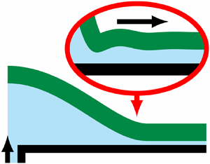
The spreading under an elastic sheet has been studied with various physical mechanisms at the moving front, including a pre-wetting film (e.g. Lister, Peng & Neufeld Reference Lister, Peng and Neufeld2013; Hewitt, Balmforth & De Bruyn Reference Hewitt, Balmforth and De Bruyn2015), a fluid lag (e.g. Hewitt et al. Reference Hewitt, Balmforth and De Bruyn2015; Ball & Neufeld Reference Ball and Neufeld2018; Wang & Detournay Reference Wang and Detournay2018) and elastic fracture (e.g. Bunger & Cruden Reference Bunger and Cruden2011; Wang & Detournay Reference Wang and Detournay2018; Lister, Skinner & Large Reference Lister, Skinner and Large2019), and sometimes with additional complications such as surface tension between two phases (e.g. Peng et al. Reference Peng, Pihler-Puzović, Juel, Heil and Lister2015) or adhesive forces between the boundaries (e.g. Ball & Neufeld Reference Ball and Neufeld2018). We focus on spreading over a pre-wetting layer of thickness  $h_0$, as shown in figure 1. This set-up can also be interpreted as injection in an elastic-walled Hele-Shaw cell, which has been studied by e.g. Pihler-Puzović et al. (Reference Pihler-Puzović, Illien, Heil and Juel2012) and Pihler-Puzović et al. (Reference Pihler-Puzović, Peng, Lister, Heil and Juel2018) in the context of controlling the Saffman–Taylor viscous-fingering instability.

Figure 1. Schematic figure of fluid injected under an elastic sheet with either two-dimensional or axisymmetric geometry.
Some aspects of this system have been studied theoretically (Flitton & King Reference Flitton and King2004; Lister et al. Reference Lister, Peng and Neufeld2013; Hewitt et al. Reference Hewitt, Balmforth and De Bruyn2015) using the method of matched asymptotic expansions, exploiting the separation of length scales between the large central ‘blister’ of fluid, where viscous forces can be neglected, and the small ‘peeling region’ near the apparent contact line, where viscous forces are important. In the blister, the viscous pressure drop is asymptotically negligible, so the blister has a quasi-static shape analogous to the spherical-cap shape of a capillary droplet. The peeling region has a travelling-wave solution, moving outwards at some speed  $\dot R = \mathrm {d}R/\mathrm {d}t$. If either bending stresses or tension forces alone are dominant, then the peeling speed depends on the apparent curvature $\kappa = \mathrm {d}^2h/\mathrm {d}x^2$ or slope $\alpha = -\mathrm {d}h/\mathrm {d}x$ at the edge of the blister solution according to the ‘peeling-by-bending’ or ‘peeling-by-pulling’ laws (see e.g. Lister et al. Reference Lister, Peng and Neufeld2013)
 \begin{equation} \dot R = 0.472\frac{B h_0^{1/2} \kappa^{5/2}}{12\mu} \quad \text{or} \quad \dot R = \frac{T \alpha^3}{12\mu \ln[(R/\ell_{p})^3]}, \end{equation}
respectively, where  $\mu$ is the dynamic viscosity of the fluid, $B$ is the bending stiffness of the sheet, $T$ is the tension in the sheet and $\ell _{p}$ is the length scale of the peeling region. (The peeling-by-pulling law (1.1b) is the elastic analogue of the Cox–Voinov law (Voinov Reference Voinov1976; Cox Reference Cox1986) for capillary spreading.) Integration of the resulting differential equation then yields the spreading law $R(t)$ for the blister at late times when any initial transient behaviour has become irrelevant.
The aim of this paper is to unify and extend the work by Lister et al. (Reference Lister, Peng and Neufeld2013) and Hewitt et al. (Reference Hewitt, Balmforth and De Bruyn2015). These studies considered various, but not all, combinations of bending, tension and gravitational forces and were restricted to the case of constant injection flux. We will, for both two-dimensional and axisymmetric geometries, systematically identify all the possible asymptotic combinations, revealing a rich variety of different behaviours. We calculate the asymptotic spreading laws  $R(t)$ for each case, while allowing fluid to be injected at an arbitrary power-law rate (which also includes the important case of constant-volume spreading).
A possible complicating factor is that the deflection of the elastic sheet also causes it to stretch and hence generates tension in the sheet, which is additional to the original constant tension imposed externally by the far-field boundary conditions. This additional tension is studied using the Föppl–von-Kármán equations in Peng & Lister (Reference Peng and Lister2020), so is assumed to be negligible here for simplicity. The condition for its neglect is discussed briefly in § 8.2.
This paper is laid out as follows. We present the governing equations in § 2. The pressure driving the flow is coupled to the liquid height by bending, tension and gravitational forces. We identify three key transition length scales that determine which combination of forces is dominant and determine the full regime diagram in § 3. We then investigate the key travelling-wave peeling solutions (§ 4), and combine them with quasi-static blister solutions to obtain asymptotic predictions for each possible combination of dominant driving forces (§ 5). The asymptotic results are verified against numerical results in § 6, and some further regimes are identified in § 7. The main points are summarized in § 8, and several generalizations of the asymptotic analysis, including to different physical controls of the peeling front, are discussed. The extraordinary variety of asymptotic results is shown in table 1, and the different regimes are shown schematically in figures 2 and 5.

Figure 2. Schematic regime diagrams showing the succession of dominant terms in (2.3) (on logarithmic axes) for the cases (a)  ${L_{TG}} \ll {L_{BT}}$ and (b) ${L_{BT}} \ll {L_{TG}}$, with ${L_{BG}} = ({L_{BT}} {L_{TG}})^{1/2}$. Main panels show which regime (combination of dominant terms) the system is in for different values of the largest scale $R$ and the smallest scale $\ell _{p}$ of the system. The arrows show possible transitions between regimes as $R(t)$ increases (moving to the right) for the case that $\ell _{p}(t)$ increases (moving upwards). The main discussion in this paper covers the unshaded areas, while the shaded areas are discussed in § 7.1. Arrows above main panels show the transition lengths (3.2) and which term dominates on a length scale $L$.
$L$.
Table 1. Summary of results in this paper for various asymptotic limits, showing the exponent  $\delta$ in $R(t) \propto t^\delta$ for various cases in two-dimensional and axisymmetric geometries with power-law injection rates (i.e. $V(t) \propto t^\beta$). See the discussion in § 8. The mechanism driving the spreading is either bending ( $B$), tension ( $T$), gravity ( $G$) or a combination as seen in figure 2. For viscously controlled peeling by pulling, there is also a logarithmic factor (indicated by an asterisk). In each column, cases with the same exponent and numerical prefactor are grouped together.

2. Governing equations
We consider the situation shown in figure 1. Viscous liquid fills the narrow gap, of initial height  $h_0$, between a horizontal rigid lower boundary and a thin overlying elastic sheet. The liquid has dynamic viscosity $\mu$ and density $\rho$, and is acted on by gravity (acceleration $g$). The sheet has bending stiffness $B = Ed^3/12(1-\nu ^2)$, where $E$ is the Young's modulus, $\nu$ is the Poisson's ratio and $d$ is the thickness of the sheet, and is also under an imposed tension $T$. We assume that these quantities are all constant.
The vertical length scales of the system are assumed to be small compared with the horizontal length scales, so that vertically integrated or averaged quantities can be employed, which are functions of the horizontal position vector  $\boldsymbol {x} = (x,y)$ and time $t$. (All vectors and tensors here have only horizontal components.) We consider both two-dimensional (2-D) and axisymmetric (axi) geometries. For the two-dimensional geometry, we assume that fluid is injected along a line source $x=0$ and spreads symmetrically in the $x$-direction. For the axisymmetric geometry, we define the radial coordinate $r = |\boldsymbol {x}|$ and assume that fluid is injected at the origin $r=0$ and spreads axisymmetrically in the $r$-direction. We use $\boldsymbol {\nabla }$ to denote the horizontal gradient operator, primes to denote differentiation with respect to the main horizontal coordinate $x$ or $r$, and overdots to denote differentiation with respect to time.
We seek to predict the evolution of the cell height profile  $h(\boldsymbol {x},t)$ (i.e. the thickness of the fluid layer), which for simplicity we often write as $h(x)$ or $h(r)$, leaving the dependence on $t$ understood. We focus in particular on the height and radius of the blister of injected fluid, defined by
 \begin{equation} {H}(t) = h(\boldsymbol{0},t), \quad R(t) = \min\{|\boldsymbol{x}| : h(\boldsymbol{x},t) = h_0\}. \end{equation}
(In (2.1b) we have chosen to define the blister radius as the distance from the origin to the closest point at which  $h=h_0$. The deflection $h-h_0$ typically has decaying oscillations in $|{\boldsymbol {x}}|>R$ and there are other reasonable choices, for example the distance to the closest minimum of $h$, but the difference is negligible at late times.)
The net upward pressure  $p_e$ on the sheet and the deflection $h - h_0$ of the sheet are coupled by the Föppl–von-Kármán equations (e.g. Landau & Lifshitz Reference Landau and Lifshitz1986), which for constant imposed tension $T$ simplify to
 \begin{equation} p_e = B\nabla^4 h - T\nabla^2 h. \end{equation}
The two terms describe, respectively, the effects of induced bending stresses (cf. the Euler beam equation) and imposed tension (cf. the Young–Laplace equation) in the sheet.
We model the viscous flow using lubrication theory (Reynolds Reference Reynolds1886). The lubrication flow is driven by horizontal gradients in the pressure field, so we can leave out pressure contributions that have no horizontal gradient, such as the atmospheric pressure, the weight of the sheet, and the vertical hydrostatic variation. The resulting effective pressure  $p(\boldsymbol {x},t)$, hereafter referred to as just ‘the pressure’, is due both to the elastic forces in the sheet and to the net hydrostatic pressure
 \begin{equation} p = p_e + \rho g h = B\nabla^4 h - T \nabla^2 h + \rho g h. \end{equation}
 We neglect any horizontal motion of the overlying sheet, and obtain a parabolic Poiseuille-flow profile. This yields the depth-integrated flux  $\boldsymbol {q}(\boldsymbol {x},t)$, from which the evolution of the height profile is found by mass conservation,
 \begin{equation} \boldsymbol{q} = -\frac{h^3}{12\mu}\boldsymbol{\nabla} p, \quad \dot h = -\boldsymbol{\nabla} \boldsymbol{\cdot}\boldsymbol{q} = \boldsymbol{\nabla} \boldsymbol{\cdot} \left(\frac{h^3}{12\mu}\boldsymbol{\nabla} p\right). \end{equation}
Equations (2.3) and (2.4) are supplemented by far-field conditions for decay to the undisturbed pre-wetting film and symmetry conditions at the origin
 \begin{equation} h \to h_0,\ p \to \rho g h_0 \text{ as } x \text{ or } r \to \infty, \quad h'(0) = h'''(0) = 0. \end{equation}
The volume  $V(t)$ of injected fluid is assumed to follow a power law,
 \begin{equation} \text{2-D: } \int_0^\infty (h - h_0)\,\,\mathrm{d} x = V(t) = Qt^\beta, \quad \text{Axi: } \int_0^\infty (h-h_0)\,2\pi r\,\,\mathrm{d} r = V(t) = Qt^\beta, \end{equation}
with an injection exponent  $\beta \geq 0$. (In the two-dimensional case, $V(t)$ denotes the volume per unit width in the third dimension in the region $x \geq 0$, which is half the total amount by symmetry.) The injection flux at the origin is thus given by
 \begin{equation} \text{2-D: } q_x = -\frac{h^3}{12\mu}p' = \dot V \text{ at } x = 0, \quad \text{Axi: } q_r = -\frac{h^3}{12\mu}p' \sim \frac{\dot V}{2\pi r} \text{ as } r \to 0. \end{equation}
We use the initial condition  $h = h_0$ at $t=0$, except that for $\beta = 0$ (constant volume) the injected volume is initially localized to a very small region near the origin.
3. Scaling analysis and transition lengths
We first need to determine which of bending, tension and gravity are dominant, and which can be neglected. In a region with height scale  $H$ and length scale $L$, the scales for the bending, tension and gravitational pressure terms in (2.3) are
 \begin{equation} p \sim \frac{BH}{L^4}, \ \frac{TH}{L^2}\quad \text{and}\quad \rho g H, \end{equation}
respectively. Balancing these pairwise reveals three key length scales which we term the bending–tension length, the bending–gravity length and the tension–gravity length, respectively,
 \begin{equation} {L_{BT}} = (B/T)^{1/2}, \quad {L_{BG}} = (B/\rho g)^{1/4}, \quad {L_{TG}} = (T/\rho g)^{1/2}. \end{equation}
These length scales are analogous to the capillary length  $(\gamma /\rho g)^{1/2}$ for capillary spreading. The bending term dominates on small length scales ( $L \ll {L_{BT}}, {L_{BG}}$), the gravity term dominates on large length scales ( $L \gg {L_{BG}}, {L_{TG}}$) and the tension term dominates on medium length scales ( ${L_{BT}} \ll L \ll {L_{TG}}$, if this interval exists).
Since  ${L_{BG}} = ({L_{BT}} {L_{TG}})^{1/2}$ lies between ${L_{BT}}$ and ${L_{TG}}$, the three transition lengths can only be ordered either as ${L_{TG}} \leq {L_{BG}} \leq {L_{BT}}$ or as ${L_{BT}} \leq {L_{BG}} \leq {L_{TG}}$. Thus, there are two asymptotic limits to consider: If ${L_{TG}} \ll {L_{BG}} \ll {L_{BT}}$ (or equivalently $T^2 \ll B\rho g$), then bending is dominant for $L \ll {L_{BG}}$ and gravity is dominant for ${L_{BG}} \ll L$, as shown in figure 2(a), while tension is always negligible. On the other hand, if ${L_{BT}} \ll {L_{BG}} \ll {L_{TG}}$ (or equivalently $T^2 \gg B\rho g$), then bending is dominant for $L \ll {L_{BT}}$, tension is dominant for ${L_{BT}} \ll L \ll {L_{TG}}$, and gravity is dominant for ${L_{TG}} \ll L$, as shown in figure 2(b).
At any given time, the horizontal length scales in the system span the range from the large blister radius  $R(t)$ down to the small length scale $\ell _{p}(t)$ of the peeling region (see § 4), which can be represented as a point $(R, \ell _{p})$ in a two-dimensional regime diagram (figure 2). The diagram can then be divided into regimes according to which forces are dominant, which is determined by how $\ell _{p}$ and $R$ compare to the transition lengths ${L_{BT}}$, ${L_{BG}}$ and ${L_{TG}}$.
In figure 2(a), for example, if both  $\ell _{p}$ and $R$ are smaller than ${L_{BG}}$, then all length scales in the system are too, so only bending forces are dominant. We refer to this regime as the ‘pure’ bending regime. Similarly, if both are larger than ${L_{BG}}$, then only gravity is dominant. However, if $\ell _{p} \ll {L_{BG}} \ll R$, then bending is dominant in the parts of the system where the length scale is $\ll {L_{BG}}$, while gravity is dominant in the parts where the length scale is $\gg {L_{BG}}$, so we have a ‘hybrid’ bending–gravity regime.
Since the fluid spreads and  $R(t)$ increases with time, the system moves towards the right in the regime diagram (figure 2). For ease of discussion, we focus on the case where $\ell _{p}(t)$ also increases with time, so that the system also moves upwards in the diagram. We shall see that this case corresponds to a decreasing peeling speed $\dot R$ and thus to a condition that the injection exponent $\beta$ is not too large. (For sufficiently large $\beta$, $\dot R$ increases and $\ell _p(t)$ decreases with time, and the system moves downwards in the diagram instead.) Moving rightwards and upwards in the diagram, the system generally evolves from being purely bending dominated at very early times to being purely gravity dominated at very late times, passing through a number of intervening hybrid, or possibly tension-dominated, regimes at intermediate times.
Since  $R(t)$ and $\ell _{p}(t)$ are not known a priori, our approach is to solve for each regime first, before determining its temporal range of validity. In § 4 we analyse the peeling region on the scale $\ell _{p}$, and in § 5 we analyse the blister shape and determine the spreading law $R(t)$ in the various regimes.
4. Travelling-wave peeling solutions
We consider the asymptotic limit  $h_0 \ll {H}$ where the pre-wetting layer is very thin relative to the thickness of the fluid that has been injected. This results in different parts of the system having asymptotically different scales, as shown in figure 3. The blister $x < R$ (or $r < R$) is the largest region, with height ${H}(t)$ and radius $R(t)$. Near its edge $x \approx R$ (or $r \approx R$) at the apparent contact line we expect to find a peeling region with height scale $h_0 \ll {H}$ and some length scale $\ell _{p}(t) \ll R$ to be determined.

Figure 3. Schematic figure of the asymptotic structure. The large blister has a small peeling region at its edge  $x=R$ or $r=R$. For the hybrid cases where multiple driving forces are dominant, the peeling region is nested inside an intermediate region (dashed arrows). The variables $h_{b}$, $h_{p}$ and $h_{i}$ and local coordinates $x_{p}$ and $x_{i}$ are used to describe the leading-order asymptotic solutions in each region.
In the peeling region, we define the leading-order solution  $h = h_{p}(x_{p})$, where $x_{p} = R(t) - x$ or $x_{p} = R(t) - r$ is an inward-pointing local coordinate. The scaling $x_{p} \sim \ell _{p} \ll R$ allows two approximations. Firstly, regardless of the global geometry (2-D or axi), the leading-order local peeling process is two-dimensional, with no variation in the horizontal direction transverse to the direction of motion. Secondly, in the time derivative $\partial h/\partial t = \partial h_{p}/\partial t + \dot R\,\partial h_{p}/\partial x_{p}$ the second term, due to the outward spreading motion, is dominant by a factor of order $R/\ell _{p}$ (assuming that $\dot R \sim R/t$). Neglecting the first term allows the governing equation (2.4b) to be integrated once, with far-field condition $h_{p}(-\infty) = h_0$, to yield the travelling-wave equation
 \begin{equation} \dot R(h_{p} - h_0) = \frac{h_{p}^3}{12\mu}\left(B h_{p}''''' - T h_{p}''' + \rho g h_{p}'\right). \end{equation}
 Given the value of  $\dot R$, the peeling length scale $\ell _{p}$ is determined by balancing the terms on the left-hand side with the relevant term or terms on the right-hand side. If one of the three terms is dominant, then $\ell _{p}$ is given by one of the expressions
 \begin{equation} \ell_{{p}{B}} = \left(\frac{B h_0^3}{12\mu \dot R}\right)^{1/5}, \quad \ell_{{p}{T}} = \left(\frac{T h_0^3}{12\mu \dot R}\right)^{1/3}, \quad \ell_{{p}{G}} = \frac{\rho g h_0^3}{12\mu \dot R}. \end{equation}
Which of these expressions is the relevant one is determined by comparing them to the transition length scales (3.2). For example, if  $\dot R$ is very large, then all the options in (4.2) are smaller than ${L_{BG}}$ and ${L_{BT}}$, so the only self-consistent possibility is that bending is dominant and $\ell _{p} = \ell _{{p}{B}}$. As $\dot R$ decreases, the length scales all increase and either tension becomes dominant instead due to both $\ell _{{p}{B}}$ and $\ell _{{p}{T}}$ crossing ${L_{BT}}$, leading to $\ell _{p} = \ell _{{p}{T}}$, or gravity becomes dominant instead due to both $\ell _{{p}{B}}$ and $\ell _{{p}{G}}$ crossing ${L_{BG}}$, leading to $\ell _{p} = \ell _{{p}{G}}$.
When a single term on the right-hand side of (4.1) is dominant, we can introduce the non-dimensionalization  $h_{p} = h_0 F(X \equiv x_{p}/\ell _{p})$, which yields the travelling-wave equations
 \begin{equation} F - 1 = F^3 F''''', \quad F-1 = -F^3 F''', \quad F-1 = F^3 F', \end{equation}
for bending, tension and gravity, respectively. These are supplemented by the far-field condition and a choice of origin
 \begin{equation} F \to 1 \text{ as } X \to -\infty, \quad 0 = \max\{X: F(X) = 1\}, \end{equation}
from (2.5a) and (2.1b), respectively, as well as suitable matching conditions to the blister as  $X \to \infty$, as stated below.
4.1. Peeling by bending
For the fifth-order peeling-by-bending equation (4.3a), the condition (4.4a) excludes two growing solutions and (4.4b) is a third condition, so we can further impose the two far-field conditions
 \begin{equation} F'''',\ F''' \to 0 \text{ as } X \to \infty, \end{equation}
which excludes the generic quartic growth of solutions to (4.3a) in favour of a slower quadratic growth. This yields a unique solution, which can be calculated numerically (Lister et al. Reference Lister, Peng and Neufeld2013) and is shown in figure 4(a). The solution has a quadratic far-field behaviour  $F'' \to C_{p}$ as $X \to \infty$, with $C_{p} \approx 1.350507$. In order to match, the leading-order blister solution $h = h_{b}$ must also have a quadratic behaviour near the apparent contact line, i.e. satisfy clamped conditions and have a non-zero curvature $\kappa$,
 \begin{equation} h_{b}(R) = h_{b}'(R) = 0, \quad \kappa = h_{b}''(R). \end{equation}
(These conditions are seen in § 5 to yield a unique solution for the blister, and matching to a different peeling solution with quartic or cubic far-field behaviour would not be possible.) Matching the curvature at the edge of the blister to that of the peeling solution yields
 \begin{equation} \kappa = C_{p} \frac{h_0}{\ell_{{p}{B}}^2} \Rightarrow \dot R = 0.471800 \frac{B h_0^{1/2}}{12\mu} \kappa^{5/2}, \end{equation}
from (4.2a), as stated in (1.1a).

Figure 4. Asymptotic travelling-wave peeling solutions for (a) bending (showing the rescaled height  $F$, curvature $F''$ and pressure $F''''$), (b) tension (showing the rescaled height $F$, slope $F'$ and pressure $-F''$) and (c) gravity (showing the rescaled height or pressure $F$).
$F$).
4.2. Peeling by pulling
For the third-order peeling-by-pulling equation (4.3b), the condition (4.4a) excludes one growing solution and (4.4b) is a second condition, so we can further impose (in analogy with (4.5)) the one condition that
 \begin{equation} F'' \to 0 \text{ as } X \to \infty. \end{equation}
This yields a unique solution, which can be calculated numerically and is shown in figure 4(b). The leading-order far-field behaviour can be determined analytically from the large- $F$ approximation of (4.3b), $1 \approx -F^2 F'''$, as
 \begin{equation} F \sim X (3\ln X)^{1/3}, \quad F' \sim (3\ln X)^{1/3} \quad \text{as } X \to \infty. \end{equation}
The far-field slope  $F'$ varies with $X$, but logarithmically slowly, so, in matching with the blister region with length scale $R$, we can use the value of $F'$ evaluated at $X = R/\ell _{{p}{T}}$.
In order for the blister solution to match the approximately linear behaviour (4.9), we require zero height and a non-zero slope  $\alpha$ near the contact line,
 \begin{equation} h_{b}(R) = 0, \quad \alpha = -h_{b}'(R). \end{equation}
Comparison with (4.9) evaluated at  $X = R/\ell _{{p}{T}}$ yields
 \begin{equation} \alpha = \left(3 \ln \frac{R}{\ell_{{p}{T}}}\right)^{1/3} \frac{h_0}{\ell_{{p}{T}}} \Rightarrow \dot R = \frac{T \alpha^3}{12\mu\,\ln[(R/\ell_{{p}{T}})^3]}, \end{equation}
as given in (1.1b). This expression has a weak logarithmic dependence on  $\ell _{{p}{T}}$ and hence on $\dot R$. In order to solve for $\dot R$ explicitly, we can make use of the Lambert $W$-function, which we denote by $\ln _*(x)$ due to its similarity with $\ln (x)$. This is defined by
 \begin{equation} \ln_*(x) \textrm{e}^{\ln_*(x)} = x, \quad \ln_*(x) = \ln x + O(\ln \ln x) \text{ as } x \to \infty. \end{equation}
We then obtain, from (4.11) and (4.2b),
 \begin{equation} \dot R = \frac{T\alpha^3}{12\mu\,\ln_*[(R\alpha/h_0)^3]}. \end{equation}
4.3. Peeling by gravitational spreading
For the first-order gravity-current equation (4.3c), the peeling process is simply gravitational spreading of the fluid under the sheet. The general solution is given implicitly by
 \begin{equation} X - X_0 = \ln(F - 1) + F + \frac{F^2}{2} + \frac{F^3}{3}, \end{equation}
which automatically satisfies the condition (4.4a) leaving only the choice of origin  $X_0$. In this case, the origin cannot be chosen using (4.4b) since $F>1$ everywhere (the solution approaches $F=1$ monotonically rather than in an oscillatory manner as $X \to -\infty$), but we can instead choose, for example, $F(0) = 1.1$, which corresponds to $X_0 \approx 0.154$. This solution is shown in figure 4(c).
For matching with the blister solution, we would expect, by analogy with the bending and tension cases, to use just the height  $F$. Requiring $h_{b}$ to match the cube-root behaviour $F \sim (3X)^{1/3}$ as $X \to \infty$ yields
 \begin{equation} \dot R = -\frac{\rho g}{12\mu} h_{b}^2(R) h_{b}'(R), \end{equation}
which describes conservation of flux at the apparent contact line.
5. Quasi-static blister solutions and resulting spreading rates
For peeling by bending (4.7) and peeling by pulling (4.13), the peeling speed  $\dot R$ decreases as $h_0$ decreases, and a posteriori scaling analyses (see § 7) show that if $h_0 \ll {H}$ then the spreading is sufficiently slow that the pressure drop in the bulk of the large blister is asymptotically negligible. The large blister region then evolves quasi-statically and its shape can be determined analytically. In this section, we perform these calculations and use (4.7) and (4.13) to obtain the spreading rate $R(t)$ in the various regimes shown in the regime diagrams in figure 2 (but restricted to the unshaded areas). We also discuss the non-quasi-static gravity-dominated case in § 5.8.
5.1. The general blister solution
We assume that the viscous pressure drop in the bulk of the blister is asymptotically negligible, and hence the pressure in the blister is spatially uniform,  $p = p_{b}(t)$, to leading order. Equivalently, pressure variations in the blister region are quickly equilibrated, owing to the large mobility $h^3/12\mu$ in the blister, and hence on the much slower time scale of spreading the pressure is approximately uniform.
The asymptotic leading-order blister solution  $h = h_{b}$ is thus obtained by solving the equation
 \begin{equation} p_{b}(t) = B\nabla^4 h_{b} - T \nabla^2 h_{b} + \rho g h_{b}, \end{equation}
(where some of the terms on the right-hand side may be negligible) with a simplified volume constraint (2.6),
 \begin{equation} \text{2-D: } \int_0^R h_{b}\,\,\mathrm{d} x = V(t) = Qt^\beta, \quad \text{Axi: } \int_0^R h_{b}\, 2\pi r\,\,\mathrm{d} r = V(t) = Qt^\beta, \end{equation}
symmetry conditions (2.5b),
 \begin{equation} h_{b}'(0) = h_{b}'''(0) = 0, \end{equation}
and suitable matching conditions to the peeling solution at the apparent contact line  $x=R$ or $r=R$ as follows.
For peeling by bending (§ 4.1), where the fourth-order bending term in (5.1) is dominant near the contact line, we use the conditions  $h_{b}(R) = h_{b}'(R) = 0$ from (4.6). For peeling by pulling (§ 4.2), where the second-order tension term in (5.1) is dominant near the contact line (and hence the fourth-order term is negligible everywhere), we use the condition $h_{b}(R) = 0$ from (4.10). Finally, if gravity is dominant near the contact line (§ 4.3), then it turns out that the blister is not quasi-static (see § 5.8).
The general solutions of the blister equations (5.1)–(5.3) with these boundary conditions involve hyperbolic or Bessel functions. The expressions are given in appendix B and some representative results are shown in figure 5. The solutions yield the curvature  $\kappa$ or slope $\alpha$ at the edge of the blister in terms of $R$,
$R$,  $t$ and the parameters of the system, which when combined with the peeling-by-bending (4.7) or peeling-by-pulling (4.13) law for $\dot R$ can be integrated to yield $R(t)$. However, in order to understand the physics better, we solve the blister equations here using asymptotic methods in each of the regimes indicated in figure 2 to obtain the relevant values of $\kappa$ or $\alpha$ as well as power-law expressions for $R(t)$ in each regime.

Figure 5. Representative two-dimensional quasi-static blister height profiles, comparing the full solutions (B 1) and (B 2) (solid curves) and the asymptotic solutions (dashed curves). The regime name, subsection and values of  $({L_{BT}}/R,{L_{BG}}/R,{L_{TG}}/R)$ for each case are (a) ‘ $B$’, § 5.2, (5,5,5); (b) ‘ $T$’, § 5.3, (0,0,5); (c) ‘ $B+T$’, § 5.4, (0.1,1,10); (d) ‘ $T+G$’, § 5.5, (0,0,0.1); (e) ‘ $B+G$’, § 5.6, (0.01,0.1,1); (f) ‘ $B+T+G$’, § 5.7, (0.04, $0.2^{3/2}$,0.2). The asymptotic solutions are given by the main blister solutions (5.4), (5.6) and composites (5.11), (5.14), (5.16) and (5.18). The letters indicate which term dominates in the bulk of the blister, in the peeling region, and in an intermediate region (if present). The key quantities – curvature $\kappa = h''$ (associated with bending), slope $\alpha = -h'$ (associated with tension) and height $\zeta = h$ (associated with gravity) – are labelled.
5.2. Bending only (regime ‘ $B$’)
$B$’)

First, if  $R \ll {L_{BG}},{L_{BT}}$ then bending is dominant everywhere and (5.1) reduces to $p_{b} = B\nabla ^4 h_{b}$. Together with (5.2), (5.3) and (4.6), this yields the blister profile $h_{b}$, pressure $p_{b}$ and peeling curvature $\kappa = h_{b}''(R)$ as
 \begin{gather} \text{2-D: } h_{b} = \frac{15}{8} \frac{V}{R} \left(1 - \frac{x^2}{R^2}\right)^2, \quad \frac{p_{b}}{B} = 45\frac{V}{R^5}, \quad \kappa = 15\frac{V}{R^3}, \end{gather}
 \begin{gather}\text{Axi: } h_{b} = \frac{3}{\pi} \frac{V}{R^2} \left(1 - \frac{r^2}{R^2}\right)^2, \quad \frac{p_{b}}{B} = \frac{192}{\pi} \frac{V}{R^6}, \quad \kappa = \frac{24}{\pi} \frac{V}{R^4}, \end{gather}
in agreement with the sample solution of (B 1) shown in figure 5(a).
We substitute the curvature  $\kappa$ into the peeling-by-bending law (4.7) and integrate the differential equation to find the spreading rate
 \begin{gather} \text{2-D: } \dot R = 411 \frac{B h_0^{1/2} Q^{5/2}t^{5\beta/2}}{12\mu R^{15/2}} \Rightarrow R(t) = 2.83\left(\frac{B^2 h_0 Q^5 t^{5\beta+2}}{(5\beta+2)^2 (12\mu)^2}\right)^{1/17}, \end{gather}
 \begin{gather}\text{Axi: } \dot R = 76.1\frac{B h_0^{1/2} Q^{5/2}t^{5\beta/2}}{12\mu R^{10}} \Rightarrow R(t) = 1.96\left(\frac{B^2 h_0 Q^5 t^{5\beta+2}}{(5\beta+2)^2 (12\mu)^2}\right)^{1/22}. \end{gather}
In this case and the following ones, once the spreading rate  $R(t)$ is known, the blister height ${H}(t)$ and pressure $p_{b}(t)$ can be calculated from the appropriate blister solution if required.
5.3. Tension only (regime ‘$T$’)

If  ${L_{BT}} \ll (R,\ell _{p}) \ll {L_{TG}}$, then tension is dominant everywhere. Equation (5.1) reduces to $p_{b} = -T\nabla ^2 h_{b}$, which is of lower order than (5.1), so we can only impose a single symmetry condition $h_{b}'(0) = 0$, together with $h_{b}(R) = 0$. The solution, which has a slope $\alpha = -h_{b}'(R)$ at the edge, is
 \begin{gather} \text{2-D: } h_{b} = \frac{3}{2}\frac{V}{R}\left(1 - \frac{x^2}{R^2}\right), \quad \frac{p_{b}}{T} = 3\frac{V}{R^3}, \quad \alpha = 3\frac{V}{R^2}, \end{gather}
 \begin{gather}\text{Axi: } h_{b} = \frac{2}{\pi} \frac{V}{R^2}\left(1 - \frac{r^2}{R^2}\right), \quad \frac{p_{b}}{T} = \frac{8}{\pi} \frac{V}{R^4}, \quad \alpha = \frac{4}{\pi}\frac{V}{R^3}, \end{gather}
in agreement with figure 5(b).
Substitution of  $\alpha$ into the peeling-by-pulling law (4.13) yields a differential equation for $R(t)$, which can be integrated at leading order by approximating the logarithmic factor $\ln _*$ in (4.13) as a constant. The leading-order result is
 \begin{gather} \text{2-D: } R(t) = 2.29\left(\frac{T Q^3 t^{3\beta+1}}{(3\beta+1) 12\mu\,\ln_*[(12\mu Q^{4} t^{4\beta-1}/T h_0^{7})^{3/4}]}\right)^{1/7}, \end{gather}
 \begin{gather}\text{Axi: } R(t) = 1.48\left(\frac{T Q^3 t^{3\beta+1}}{(3\beta+1)12\mu\,\ln_*[(12\mu Q^{2}t^{2\beta-1}/T h_0^{5})^{3/2}]}\right)^{1/10}. \end{gather}
We have neglected an  $O(1)$ numerical factor inside the argument of each $\ln _*$ in (5.7) as it represents only a higher-order correction. Determining the values of these $O(1)$ factors requires not only more careful integration of the differential equation, but also evaluation of corrections to the blister solution (due to the viscous pressure drop in the blister) and to the far-field behaviour of the peeling solution; the details are somewhat complicated and are given in appendix C.
5.4. Bending and tension (regime ‘$B+T$’)

When  $\ell _{p} \ll {L_{BT}} \ll R \ll {L_{TG}}$, bending is dominant on the peeling length scale $\ell _{p} = \ell _{{p}{B}}$, while tension is dominant on main scale $R$ of the blister. Hence, the peeling-by-bending solution (4.7) and the tension-dominated blister solution (5.6) apply. Since this blister solution has a non-zero slope $\alpha = -h'(R)$, it does not satisfy the clamping condition $h'(R) = 0$ required for direct matching, so there must be an intermediate region near the apparent contact line, on the length scale ${L_{BT}}$ where tension and bending balance.
For the intermediate solution, we define the leading-order solution  $h_{i}$ and local coordinate $x_{i}$ (which is equal to $x_{p}$) by
 \begin{equation} h = h_{i}(x_{i}), \quad x_{i} = R(t) - x \text{ (2-D)}\quad \text{or} \quad x_{i} = R(t) - r \text{ (axi)}. \end{equation}
In the blister equation (5.1), the constant pressure  $p_{b} \sim T \alpha /R$ is set by the main solution (5.6). This pressure is negligible on the intermediate scale, where the bending and tension terms are much larger, scaling like $T\alpha /{L_{BT}}$ (from $x_{i} \sim {L_{BT}} \ll R$ and $h_{i} \sim \alpha x_{i}$). Thus, the leading-order problem on the intermediate scale is
 \begin{equation} B h_{i}'''' - Th_{i}'' = 0, \quad h_{i}(0) = h_{i}'(0) = 0, \quad h_{i}'(\infty) = \alpha, \end{equation}
representing the role of bending in effecting the transition from clamped conditions at  $x_{i} = 0$ to a non-zero slope $\alpha$ as $x_{i} \to \infty$. The unique solution of (5.9) is (e.g. Lister et al. Reference Lister, Peng and Neufeld2013)
 \begin{equation} h_{i}(x_{i}) = \alpha{L_{BT}} \left[\frac{x_{i}}{{L_{BT}}} + (\textrm{e}^{-x_{i}/{L_{BT}}} - 1)\right], \quad \kappa = h_{i}''(0) = \frac{\alpha}{{L_{BT}}}. \end{equation}
For comparison with the full solution (B 1), we can form composite solutions of (5.6) and (5.10). For the two-dimensional case, after rescaling by the blister height, the additive composite is given by
 \begin{equation} h = {H} \frac{1 - (x/R)^2 + 2 ({L_{BT}}/R)(\textrm{e}^{-(R - x)/{L_{BT}}} - 1)}{1 + 2({L_{BT}}/R)(\textrm{e}^{-R/{L_{BT}}} - 1)}, \end{equation}
and is in good agreement with the full solution, as shown in figure 5(c). The axisymmetric case can be treated similarly.
The effect of the bending–tension intermediate solution is to convert the slope  $\alpha$ given by the main blister solution (5.6) to a curvature $\kappa = \alpha /{L_{BT}}$ that matches with the peeling region. Substitution into the peeling-by-bending law (4.7) yields, after integration,
 \begin{gather} \text{2-D: } R(t) = 2.11\left(\frac{T^5 h_0^2 Q^{10} t^{10\beta+4}}{(5\beta+2)^4(12\mu)^4 B}\right)^{1/24}, \end{gather}
 \begin{gather}\text{Axi: } R(t) = 1.37\left(\frac{T^5 h_0^2 Q^{10} t^{10\beta+4}}{(5\beta+2)^4 (12\mu)^4 B}\right)^{1/34}. \end{gather}
For this and the other hybrid solutions calculated below in § 5, the results only apply in the unshaded areas of the regime diagram (figure 2), as the assumption that the pressure is approximately uniform throughout the blister fails in the shaded areas. We discuss this issue further in § 7.
5.5. Tension and gravity (regime ‘$T+G$’)

Gravity is dominant on the main scale  $R$ of the blister if $R \gg {L_{BG}},{L_{TG}}$. This reduces (5.1) to the trivial equation $p_{b} = \rho g h_{b}$, resulting in a flat-topped profile with constant height $\zeta$,
 \begin{equation} \text{2-D: } h_{b}(x) = \frac{p_{b}}{\rho g} = \zeta = \frac{V}{R}, \quad \text{Axi: } h_{b}(r) = \frac{p_{b}}{\rho g} = \zeta = \frac{1}{\pi}\frac{V}{R^2}, \end{equation}
which again agrees with (B 1) and figure 5(d–f). However, this solution cannot match (4.6) or (4.10) directly.
If  ${L_{BT}} \ll \ell _{{p}} \ll {L_{TG}} \ll R$, then tension dominates in the peeling region (while bending is negligible everywhere). At the edge of the gravity-dominated blister (5.13), there is need for a tension–gravity intermediate solution $h_{i}(x_{i})$ on the scale ${L_{TG}}$, which satisfies $-T h_{i}'' + \rho g h_{i} = p_{b} = \rho g \zeta$ with the condition $h_{i}(0) = 0$ and the matching condition $h_{i}(\infty) = \zeta$ to (5.13). The solution is
 \begin{equation} h_{i}(x_{i}) = \zeta\left[1 - \textrm{e}^{-x_{i}/{L_{TG}}}\right], \quad \alpha = h_{i}'(0) = \frac{\zeta}{{L_{TG}}}, \end{equation}
which converts the height  $\zeta$ into the slope $\alpha$, as illustrated in figure 5(d) (where (5.14) is used as asymptotic composite of (5.14) and (5.13), with a rescaling). Substitution of $\alpha$ into the peeling-by-pulling law (4.13) with the length scale ${L_{TG}}$ instead of $R$ in the argument of $\ln _*$ yields, after integration,
 \begin{gather} \text{2-D: } R(t) = 2.00\left(\frac{(\rho g)^{3/2} T^{-1/2} Q^3 t^{3\beta+1}}{(3\beta+1)\,12\mu\,\ln_*[(12\mu)^3 T^{3/2} Q^3 t^{3\beta-3}/(\rho g)^{9/2}h_0^{12}]}\right)^{1/4}, \end{gather}
 \begin{gather}\text{Axi: } R(t) = 1.07 \left(\frac{(\rho g)^{3/2} T^{-1/2} Q^3 t^{3\beta+1}}{(3\beta+1)\,12\mu\,\ln_*[(12\mu)^6 T^3 Q^3 t^{3\beta-6}/(\rho g)^9 h_0^{21}]}\right)^{1/7}. \end{gather}
(In this case, the next-order corrections due to the viscous pressure drop in the flat-topped part of the blister are of relative order  $O(12\mu R^3/{H}^3 t)$, which turns out to be much greater than the effect of changing the argument of $\ln _*$ by a $O(1)$ constant or indeed replacing $\ln _*(\cdot)$ with $\ln (\cdot)$. Due to the effect to be discussed in § 7.1, this regime has a rather small range of validity, so we do not calculate the corrections in more detail.)
5.6. Bending and gravity (regime ‘$B+G$’)

If  $\ell _{p} \ll {L_{BG}} \ll R$ and $T^2 \ll \rho g B$ (figure 2a), then gravity dominates in the blister and bending dominates in the peeling region (while tension is negligible everywhere). This leads to a bending–gravity intermediate solution $h_{i}(x_{i})$ on the scale $x_{i} \sim {L_{BG}}$, satisfying $B h_{i}'''' + \rho g h_{i} = p_{b} = \rho g \zeta$ with the clamped conditions $h_{i}(0) = h_{i}'(0) = 0$ and the matching condition $h_{i}(\infty) = \zeta$. The unique solution is (e.g. Bunger & Cruden Reference Bunger and Cruden2011)
 \begin{equation} h_{i} = \zeta\left[1 - \textrm{e}^{-{x_{i}}/{\sqrt{2}{L_{BG}}}}\left(\cos \frac{x_{i}}{\sqrt2 {L_{BG}}} + \sin\frac{x_{i}}{\sqrt2 {L_{BG}}}\right)\right], \quad \kappa = h_{i}''(0) = \frac{\zeta}{{L_{BG}}^2}, \end{equation}
which converts the height  $\zeta$ of the gravity-dominated blister solution (5.13) into a curvature $\kappa$ at the edge as shown in figure 5(e) (where (5.16) is used as asymptotic composite of (5.16) and (5.13), with a rescaling).
Substitution of (5.13) and (5.16) into the peeling-by-bending law (4.7) yields, after integration,
 \begin{gather} \text{2-D: } R(t) = 1.41 \left(\frac{(\rho g)^5 h_0^2 Q^{10} t^{10\beta+4}}{(5\beta+2)^4(12\mu)^4 B}\right)^{1/14}, \end{gather}
 \begin{gather}\text{Axi: } R(t) = 0.829 \left(\frac{(\rho g)^5 h_0^2 Q^{10} t^{10\beta+4}}{(5\beta+2)^4 (12\mu)^4 B}\right)^{1/24}. \end{gather}
5.7. Bending, tension and gravity (regime ‘$B+T+G$’)

If instead  $T^2 \gg \rho g B$ (figure 2b), so that $\ell _{p} \ll {L_{BT}} \ll {L_{TG}} \ll R$, then we obtain a nested hierarchy of intermediate solutions as shown in figure 5(f). The gravity-dominated blister (5.13) has a constant height $\zeta$, a tension–gravity intermediate solution (5.14) converts $\zeta$ into the slope $\alpha = \zeta /{L_{TG}}$, and a bending–tension intermediate solution (5.10) converts $\alpha$ into the curvature $\kappa = \alpha /{L_{BT}}$, which then feeds into the peeling-by-bending law (4.7). The two-dimensional asymptotic composite of (5.13), (5.14) and (5.10) shown in figure 5(f) is
 \begin{equation} h = H\frac{1 - \textrm{e}^{-(R-x)/{L_{TG}}} +({L_{BT}}/{L_{TG}})(\textrm{e}^{-(R-x)/{L_{BT}}} - 1)}{1 - \textrm{e}^{-R/{L_{TG}}} + ({L_{BT}}/{L_{TG}})(\textrm{e}^{-R/{L_{BT}}} - 1)}. \end{equation}
 The relationship between  $\kappa$ and $\zeta$ is given by $\kappa = \zeta /({L_{BT}} {L_{TG}}) = \zeta /{L_{BG}}^2$, which is the same as the bending–gravity result (5.16) without the intermediate tension. Hence, the spreading rate is again given by (5.17).
5.8. Gravity only (regime ‘$G$’)

If gravity dominates everywhere, then the quasi-static solution (5.13) does not apply: It clearly does not match the cube-root behaviour (4.15), and a scaling analysis reveals that the pressure gradient is not, in fact, negligible in the blister. Instead, there is a full leading-order balance in the lubrication equation (2.4) on the blister scale, with the condition that  $h_{b} \to 0$ with conservation of flux (4.15) at the apparent contact line. At leading order, this yields the self-similar gravity-current solutions calculated by Huppert (Reference Huppert1982),
 \begin{equation} \text{2-D: } h_{b}(x) = {H}(t)\,\phi_1(x/R(t)), \quad \text{Axi: } h_{b}(r) = {H}(t)\,\phi_2(r/R(t)), \end{equation}
with the blister radius and height given by the power laws
 \begin{gather} \text{2-D: } R(t)= A_1\left(\frac{\rho g Q^3 t^{3\beta+1}}{12\mu}\right)^{1/5},\quad {H}(t) = A_2 \left(\frac{12\mu\,Q^2 t^{2\beta-1}}{\rho g}\right)^{1/5}, \end{gather}
 \begin{gather}\text{Axi: } R(t) = A_3\left(\frac{\rho g Q^3 t^{3\beta+1}}{12\mu}\right)^{1/8}, \quad {H}(t) = A_4 \left(\frac{12\mu\,Q t^{\beta-1}}{\rho g}\right)^{1/4}. \end{gather}
The profiles  $\phi _{1,2}$ and the coefficients $A_{1,2,3,4}$ depend on $\beta$ and are calculated numerically. At the apparent contact line, the nose of the gravity current (5.19) connects smoothly to the pre-wetting layer via the peeling solution (4.14).
6. Comparison with numerical results
We solved the governing equations (2.3)–(2.7) numerically using a finite-difference method; see appendix A for details. For the numerical calculations, we non-dimensionalized the equations using the scale  $h_0$ for $h$ and the bending scales
 \begin{gather} \text{2-D: } x_{B} = \left(\frac{B^\beta h_0^{3\beta+1}}{(12\mu)^\beta Q}\right)^{{1}/({6\beta-1})}, \quad t_{B} = \left(\frac{Bh_0^9}{12\mu Q^6}\right)^{{1}/({6\beta-1})}, \end{gather}
 \begin{gather}\text{Axi: } x_{B} = \left(\frac{B^\beta h_0^{3\beta+1}}{(12\mu)^\beta Q}\right)^{{1}/({6\beta-2})}, \quad t_{B} = \left(\frac{B^2 h_0^{12}}{(12\mu)^2 Q^6}\right)^{{1}/({6\beta-2})}, \end{gather}
for  $x$ or $r$ and $t$, respectively. These are obtained by balancing the pressure with the bending term in (2.3), i.e. $p \sim B h/x^4$, and then balancing all the other terms in the remaining equations (2.4)–(2.7). The resulting non-dimensionalization is equivalent to setting $B = 12\mu = Q = h_0 = 1$ and replacing the tension and gravity coefficients $T$ and $\rho g$ with non-dimensional versions
 \begin{equation} T_{B} = \frac{T x_{B}^2}{B} = \left(\frac{x_{B}}{{L_{BT}}}\right)^2, \quad G_{B} = \frac{\rho g x_{B}^4}{B} = \left(\frac{x_{B}}{{L_{BG}}}\right)^4, \end{equation}
both in the governing equations (2.3)–(2.7) and in the asymptotic results (§ 5). The coefficients  $T_{B}$ and $G_{B}$ and the injection exponent $\beta$ form a complete set of three independent parameters for this system.
We compare the asymptotic predictions for  $R(t)$ from § 5 with the corresponding numerical results in figure 6 using a compensated log–log plot where $R(t)$ is divided by a suitable power of $t$ in order to highlight the difference between regimes. We focus on the fixed value $G_{B} = 10^{-32}$ for the non-dimensional gravity, and consider three different values $T_{B} = 0,\ 10^{-10},\ 10^{-6}$ for the non-dimensional tension. These values have been chosen to be rather extreme, in order to allow the system to display clear transitions between the various regimes. We find that the transitions are very similar for the two-dimensional and axisymmetric cases, albeit with different exponents. The following discussion applies to both cases, and more generally to cases where the injection exponent $\beta$ is sufficiently small that $\ell _{p}$ increases with time.

Figure 6. Numerical results (solid curves) and asymptotic solutions (dashed curves) for (a) two-dimensional spreading with injection exponent  $\beta = 1$ and (b) axisymmetric spreading with injection exponent $\beta = 1.5$. We use the bending scales (6.1) and fix $\rho g = 10^{-32} B/x_{B}^4$, while considering three values for tension, $T = 0$, $T_1 = 10^{-10} B/x_{B}^2$ and $T_2 = 10^{-6} B/x_{B}^2$. The asymptotic results are labelled as in figures 2 and 5, with the subscripts indicating the value of $T$. The radius $R(t)$ has been divided by the power of $t$ from the bending–tension hybrid regime (5.12) in order to show more clearly the differences between the regimes. The dotted lines indicate where $R$ is equal to one of the transition lengths (3.2).
Initially, since  $T_{B} \ll 1$ and $G_{B} \ll 1$ the system is bending dominated and follows the pure-bending spreading law (5.5), labelled ‘ $B$’.
$B$’.
For the case  $T_{B} = 0$ (which corresponds to figure 2a), the bending-dominated regime lasts until the radius crosses ${L_{BG}} = 10^{-8}x_{B}$ (indicated by the dotted line). Then, gravitational forces become important and the system follows the bending–gravity hybrid solution (5.17), labelled ‘ $B+G$’. Finally, the system transitions to the gravity-current spreading law (5.20), labelled ‘ $G$’.
$G$’.
For the cases  $T_{B} = 10^{-10}$ and $10^{-6}$ (which correspond to figure 2b), the system transitions from the pure-bending regime to the bending–tension hybrid regime (5.12), labelled ‘ $B+T_{1,2}$’, as $R$ crosses ${L_{BT}}$. For $T_{B} = 10^{-10}$, when $R$ subsequently crosses ${L_{TG}}$ the system transitions to the bending–tension–gravity regime, whose spreading rate is the same as the bending–gravity regime (‘ $B+G$’), and eventually into the gravity regime (‘ $G$’). For $T_{B} = 10^{-6}$, the bending–tension regime gives way to the pure-tension regime (5.7), labelled ‘ $T_2$’. The system then follows the tension–gravity regime (5.15), labelled ‘ $T_2+G$’, briefly before transitioning to the gravity regime (‘ $G$’).
We have thus exhibited all possible transitions shown in the regime diagrams in figure 2, and found excellent agreement between the numerical results and our asymptotic predictions. For less extreme, but still small, values of  $T_{B}$ and $G_{B}$, the same transitions will happen but less clearly, while if one or both of $T_{B}$ and $G_{B}$ is large then some of the earlier regimes involving bending might not occur. Also, for larger values of $\beta$ other paths through the regime diagram might be taken.
However, a more careful investigation reveals that there are a few additional transitional regimes, indicated by the shaded areas in the regime diagrams in figure 2. We identify these by examining the validity of some of the asymptotic assumptions made.
7. Validity of assumptions
The asymptotic results presented in this paper thus far rely on several assumptions, which we shall now check a posteriori, making use of the bending scales  $x_{B}$ and $t_{B}$ (6.1) to keep the expressions simple.
Firstly, the governing elastic and lubrication equations (2.2) and (2.4) require the slope of the sheet to be small,  $h'\ll 1$, in order to be valid. Thus, the validity of the results shown in figure 6 depends on the aspect ratio $x_{B}/h_0$ of the non-dimensionalization (6.1), since the true slope $h'$ is related to the non-dimensional slope $h^{\prime *}$ by $h' = (h_0/x_{B})h^{\prime *}$. In general, any non-dimensional results in a finite time range have a maximum slope $h^{\prime *}$ and hence are valid provided that $x_{B}/h_0 \gg h^{\prime *}$. More specific bounds can be obtained for each asymptotic regime. For example, for the two-dimensional pure-bending case (5.5a), the slope is largest in the blister, with $h' \sim {H}/R \sim (h_0/x_{B})(t/t_{B})^{(7\beta -4)/17}$. Thus, for $\beta < 4/7$ the slope decreases with time and the equations are valid for $t \gg t_{B}(h_0/x_{B})^{17/(4-7\beta)}$, while for $\beta > 4/7$ the criterion is $t \ll t_{B}(x_{B}/h_0)^{17/(7\beta -4)}$.
Secondly, the height  ${H}(t)$ of the blister must satisfy ${H} \gg h_0$. Using (5.5a) as an example again, we have ${H} \sim h_0(t/t_{B})^{(12\beta -2)/17}$, so for $\beta > 1/6$ the result is valid at late times $t \gg t_{B}$, while for $\beta < 1/6$ the result is valid at early times $t \ll t_{B}$. As long as this height condition ${H} \gg h_0$ is satisfied, the separation of length scales between the large two-dimensional or axisymmetric blister and the small two-dimensional travelling-wave peeling region ( $R \gg \ell _{p}$) is also guaranteed.
Thirdly, the horizontal length scales  $\ell _{p}$ and $R$ must lie in the predicted range according to the regime diagram in figure 2. For the radius $R(t)$, the situation is straightforward. For example, in the absence of tension, the pure-bending solution (5.5) transitions to the gravity–bending solution (5.17) when gravity becomes important due to $R(t)$ crossing ${L_{BG}}$ as expected (figure 6), and this transition can also be identified by simply equating the results (5.5) and (5.17).
However, for the peeling length  $\ell _{p}(t)$ things are more complicated. For example, consider the transition from the bending–gravity regime (5.17) towards the gravity-current regime (5.20). The two-dimensional result (5.17a) yields the prediction $\ell _{{p}{B}}(t) \sim G_{B}^{-1/14} (t/t_{B})^{(1-\beta)/7} x_{B}$ for the peeling-by-bending length scale, which crosses ${L_{BG}} = G_{B}^{-1/4} x_{B}$ at the time $t \sim t_{B} G_{B}^{5/(4\beta -4)}$. However, the transition actually occurs at the time found from equating (5.17) and (5.20) as seen in figure 6,
 \begin{equation} G_{B}^{5/14} (t/t_{B})^{(5\beta+2)/7} \sim G_{B}^{1/5} (t/t_{B})^{(3\beta+1)/5} \Rightarrow t \sim G_{B}^{-11/(8\beta+6)} t_{B} . \end{equation}
Past this transition, although the peeling length is  $\ell _{p} = \ell _{{p}{B}} \ll {L_{BG}}$ and bending forces are present, the spreading rate $R(t)$ is given by the gravity-current solution (5.20).
This is because, fourthly, the asymptotic method requires viscous dissipation in the blister to be small compared with the viscous dissipation in the peeling region, so that the spreading is controlled by the peeling process. In the blister, the dissipation is due to the (slow) evolution represented by  $\dot h$ in (2.4), and results in a pressure drop that scales like ${\rm \Delta} p = 12\mu R \dot R/{H}^2$, which needs to be small compared with the blister pressure $p_{b} \sim B {H}/R^4$ in order to be negligible. For the pure-bending regime (5.5), we obtain ${\rm \Delta} p/p_{b} \sim (h_0/{H})^{1/2}$, so this condition is satisfied provided ${H} \gg h_0$. However, for the bending–gravity regime (5.17), we have $p_{b} \sim \rho g {H}$ and find that ${\rm \Delta} p/p_{b} \sim \ell _{{p}{B}} R/{L_{BG}}^2$. Thus, the condition $\ell _{{p}{B}} \ll {L_{BG}}$ is not sufficient, and instead we have the stricter condition $\ell _{{p}{B}}R \ll {L_{BG}}^2$, which agrees with the transition (7.1) above.
7.1. Additional regimes
We have thus found that when  $\ell _{{p}{B}} \ll {L_{BG}} \ll R$, so that bending and gravity dominate in the peeling and blister regions, respectively, if also $\ell _{{p}{B}}R \gg {L_{BG}}^2$ then the spreading is controlled by viscous dissipation in the bulk of the blister rather than by peeling. Hence we recover the gravity-current solution (5.20) for the blister, with a peeling-by-bending tip that has a negligible effect on the spreading rate, but which persists until $\ell _{{p}} \gg {L_{BG}}$.
We illustrate the relevant transitions in figure 7 with some snapshots from a two-dimensional numerical simulation with no tension ( $T_{B} = 0$) and weak gravity $G_{B} = 10^{-12}$, leading to a bending–gravity length scale ${L_{BG}} = 10^3 x_{B}$. (This case has been studied in more detail by Hewitt et al. (Reference Hewitt, Balmforth and De Bruyn2015).) Initially, when $x_{B} \ll R(t) \ll {L_{BG}}$, the system follows the pure-bending solution (5.5), and the profiles collapse onto the blister prediction (5.4) when rescaled by the predicted time dependence. As $R$ crosses ${L_{BG}}$, gravity becomes important and the blister becomes flatter. At $t = 10^9 t_{B}$ the profile matches the asymptotic bending–gravity solution (5.16), and then tends towards the gravity-current profile (inset of figure 7).

Figure 7. Numerical results (height profiles) for two-dimensional bending- and gravity-driven spreading with  $\beta = 1$ and $x_{B} / {L_{BG}} = G_B^{1/4} = 10^{-3}$ (see (6.1a)). The initial evolution $t/t_{B} \leq 10^9$ (main figure) is rescaled using the pure-bending asymptotic result (5.5) and the subsequent evolution $t/t_{B} \geq 10^9$ (inset) is rescaled using the pure-gravity asymptotic result (5.20). The asymptotic result (5.16) is overlaid for $t/t_{B} = 10^9$ (dashed curve).
The peeling-by-bending solution (4.7) and the bending–gravity intermediate solution (5.16) are still present near the apparent contact line, as predicted by the regime diagram (figure 2), but they do not control the spreading. Rather, the causality can be thought of as being reversed: the spreading rate  $\dot R$ set by the gravity current (5.20) determines the peeling curvature $\kappa$ (4.7), which sets the cut-off height $\zeta$ (5.16) at the front of the gravity-current solution as seen in the inset of figure 7.
This regime, where bending and gravitational forces are dominant in different regions but  $R(t)$ is given by the gravity-current result (5.20) instead of the bending–gravity hybrid result (5.17), is indicated schematically by the shaded area in figure 2(a). Similarly, in the analogous light shaded areas in figure 2(b), elastic forces are present but the leading-order solution is the gravity current (5.20). The results labelled ‘ $G$’ in figure 6 are in fact in these shaded regimes, rather than in the pure-gravity regime.
The only remaining additional regime is for the combination of bending and tension, and corresponds to the dark shaded area in figure 2(b). In the transition between peeling by bending and peeling by pulling, there is an intermediate regime that is very similar to the pure-tension regime (§ 5.3), but with the bending–tension intermediate solution (5.10) and peeling-by-bending region (4.7) providing a cutoff. In this case, the bending–tension length  ${L_{BT}}$ takes the place of the peeling-by-pulling length $\ell _{{p}{T}}$ in the logarithm in (4.11), resulting in a spreading rate that has the same main power-law behaviour as for pure tension (5.7) but with a different logarithmic factor. A scaling analysis shows that this regime has a very narrow range of validity,
 \begin{equation} \frac{R}{{L_{BT}}} \left(\ln\frac{R}{{L_{BT}}}\right)^{1/3} \ll \frac{{H}}{h_0} \ll \frac{R}{{L_{BT}}}\left(\ln\frac{R}{{L_{BT}}}\right)^2, \quad \frac{R}{{L_{BT}}} \gg 1, \end{equation}
so we do not study it further.
8. Summary and generalizations
We have investigated spreading of a large two-dimensional or axisymmetric blister of fluid in the narrow gap between a horizontal rigid base and an overlying elastic sheet, with a pre-wetting film extending ahead of the blister. The spreading is driven by various combinations of bending, tension and gravitational forces depending on the horizontal length scales of the system as shown in figure 2, and is typically controlled by viscous forces in a travelling-wave peeling region at the apparent contact line at the edge of the blister (§ 4). The blister is then described by a quasi-static solution, as shown in figure 5, which depends on which of the driving forces play a role (§ 5).
If  $R(t) \ll {L_{BG}},\ {L_{BT}}$, then the blister is bending dominated and has the profile (5.4) with given curvature $\kappa$ at its edge. The peeling speed is then given in terms of $\kappa$ by the peeling-by-bending law (4.7).
If  ${L_{BT}} \ll R(t) \ll {L_{TG}}$, then the main part of the blister is tension dominated and has the parabolic profile (5.6), with given slope $\alpha$ at its edge. If the peeling length $\ell _{{p}}(t)$ is also in the same range, then the peeling speed is given in terms of $\alpha$ by the peeling-by-pulling law (4.13). If, on the other hand, the peeling length is much shorter, then the slope $\alpha$ is converted into a curvature $\kappa$ by a bending–tension intermediate solution (5.10), and the peeling speed is given by the peeling-by-bending law (4.7).
If  $R(t) \gg {L_{BG}},\ {L_{TG}}$, then the bulk of the blister is gravity dominated and has the profile (5.13) with a constant height $\zeta$ (provided the spreading is sufficiently slow). Intermediate solutions convert the height $\zeta$ into either the curvature $\kappa$ of (5.16) for peeling by bending (4.7) or the slope $\alpha$ of (5.14) for peeling by pulling (4.13). (However, if the viscous dissipation of the elastic peeling solutions is too small, then the dissipation in the blister dominates instead, and the blister spreads like a classical viscous gravity current (5.20) despite the presence of elastic forces at the apparent contact line.)
In all the above cases, except for the gravity-current regimes, we obtain a differential equation for  $R(t)$ which is readily solved. A summary of the power laws obtained in the various cases is given in table 1, which also contains some extensions to our work as described below.
8.1. Alternative physics at the peeling front
As mentioned in § 1, the problem that a no-slip contact line cannot advance (Huh & Scriven Reference Huh and Scriven1971) can be resolved by other physical mechanisms than a pre-wetting layer. If these mechanisms are also ‘microscopic’, i.e. only have an effect on a scale much smaller than the blister, then the spreading remains controlled by the physics near the advancing contact line, and the quasi-static blister solutions calculated in § 5 still apply, but match to alternative peeling solutions at their edge.
All of the asymptotic results in this paper can be directly translated to cover other microscopic mechanisms with a fixed height scale  ${H_{p}}$, by simply replacing $h_0$ with a suitable $O(1)$ multiple of ${H_{p}}$. Two such examples are when the no-slip condition on the sheet and base are replaced by a Navier-slip condition with a small slip length $\lambda$ (e.g. Hocking Reference Hocking1983), or when the base has a porous upper layer of thickness $b$ and permeability $k$ through which the fluid also flows (e.g. Hewitt, Chini & Neufeld Reference Hewitt, Chini and Neufeld2018). For these cases, the lubrication equation (2.4a) is modified to
 \begin{equation} \boldsymbol{q} = -\frac{h^3 + 6\lambda h^2}{12\mu}\boldsymbol{\nabla} p \text{ or } \boldsymbol{q} = -\frac{h^3 + 12kb}{12\mu}\boldsymbol{\nabla} p, \end{equation}
respectively, and due to the additional mobility as  $h \to 0$, these models admit travelling-wave solutions which touch down with $h(R) = h'(R) = q(R) = 0$. After solving the peeling-by-bending equations analogous to (4.3a), we obtain the peeling speed (4.7) with $h_0$ replaced by $1.037968\lambda$ or $0.959070(kb)^{1/3}$, respectively; consequently the results (5.5), (5.12) and (5.17) for $R(t)$ simply acquire the same modification. The peeling-by-pulling results (4.13), (5.7) and (5.15), however, apply with $h_0$ replaced by $\lambda$ or $(kb)^{1/3}$ directly, since any $O(1)$ prefactor inside the $\ln _*$ has no leading-order effect, while the logarithmic corrections calculated in appendix C would need different values for ${C_p}$.
Alternatively, the viscous resistance to motion might cause the pressure near the advancing contact line to drop to a critical value  $-{P_{p}}$ (relative to the ambient) at which gases come out of solution or the liquid itself evaporates, resulting in the fluid lagging behind the point where the sheet contacts the base, and the gap between the fluid and the contact point being filled with inviscid vapour at constant pressure $-{P_{p}}$ (e.g. Hewitt et al. Reference Hewitt, Balmforth and De Bruyn2015). In this case, or any other with a fixed microscopic pressure scale, a scaling analysis for the peeling wave with a given pressure scale ${P_{p}}$ yields
 \begin{equation} \dot R \propto \frac{B^{3/2}\kappa^{7/2}}{12\mu {P_{p}}^{1/2}} \text{ or } \dot R = \frac{T\alpha^3}{12\mu \ln[(R {P_{p}}/\alpha T)^3]}, \end{equation}
for peeling by bending and peeling by pulling, respectively. The resulting power-law exponents for each regime are shown in the second column of table 1.
Another possibility is that the elastic sheet model (2.2) breaks down near the contact line, due to the horizontal peeling length scale being sufficiently small that it is comparable to the sheet thickness  $d$. In this case, the full equations of linear elasticity apply instead (e.g. Lister et al. Reference Lister, Skinner and Large2019), and, provided that the spreading is controlled by viscous dissipation on this scale, a balance in the travelling-wave equation (4.1) with $\ell _{p} = d$ yields
 \begin{equation} \dot R \propto \frac{Bd\kappa^3}{12\mu} \text{ or } \dot R = \frac{T\alpha^3}{12\mu \ln[(R/d)^3]}. \end{equation}
The resulting power-law exponents, for this case and any other with a fixed peeling length scale  $\ell _{p}$, are shown in the third column of table 1.
Finally, it is also possible that the spread of the blister is not dynamically controlled by viscous resistance, but rather (quasi-)statically controlled by a surface energy, in that increasing the peeled area (e.g.  $A = \pi R^2$ in the axisymmetric case) by a given increment $\mathrm {d}A$ requires a fixed energy $\gamma \,\mathrm {d}A$. This could be due to bonds between the sheet and the plate requiring a fracture energy to break (e.g. Lister et al. Reference Lister, Skinner and Large2019), van der Waals forces (e.g. Hosoi & Mahadevan Reference Hosoi and Mahadevan2004) or magnetic attraction (e.g. Ball & Neufeld Reference Ball and Neufeld2018). It could also be due to surface tension (with coefficient $\gamma /2$) around an injected pancake-shaped gas bubble filling the blister (e.g. Peng et al. Reference Peng, Pihler-Puzović, Juel, Heil and Lister2015). A balance between the elastic or gravitational energy released by the blister spreading and the surface-energy requirement for peeling then yields the quasi-static conditions (e.g. Landau & Lifshitz Reference Landau and Lifshitz1986)
 \begin{equation} \kappa^2 = \frac{2\gamma}{B}, \quad \alpha^2 = \frac{2\gamma}{T} \text{ or } \zeta^2 = \frac{2\gamma}{\rho g}. \end{equation}
Solving for  $R(t)$ using the blister solutions in § 5 yields the power laws shown in the fourth column of table 1.
8.2. Generalizations to other related problems
We have considered injecting the liquid with a specified volume  $V(t)$ or equivalently flux $\dot V(t)$. For an alternative injection strategy, such as a specified (effective) pressure or specified height, or something more exotic like a height-dependent injection flux (e.g. Kiradjiev, Breward & Griffiths Reference Kiradjiev, Breward and Griffiths2019), the blister solutions (5.4), (5.6) and (5.13) can be used with $V(t)$ depending on $t$ and $R$ so as to achieve the desired effect, and the new differential equations obtained for $R(t)$ can be integrated to yield the solution. Similarly, if there is a slow temporal and/or gentle spatial variation in the physics (such as the value of $h_0$) at the contact line then the peeling laws (§ 4) still apply but the final integration of the equation for $R(t)$ is different.
For spreading in two horizontal dimensions with non-axisymmetric spatial variations or initial conditions, although the blister shape cannot be solved for analytically in general, the asymptotic decomposition can still be employed to simplify the problem. Instead of fully resolving the contact-line dynamics, a numerical method can be employed to simply track the location of the contact line and solve for a quasi-static constant-pressure blister shape within it. The curvature or slope at the contact line then determines the speed at which it advances.
For a viscous fluid spreading in the thin gap between an inner rigid cylinder and an outer concentric elastic cylindrical shell (e.g. Elbaz & Gat Reference Elbaz and Gat2016), the axial evolution equation for the axisymmetric layer thickness  $h$ is given by
 \begin{equation} \dot h = \left(\frac{h^3}{12\mu}p'\right)', \quad p = Bh'''' - Th'' + \frac{Ed}{a^2}h, \end{equation}
where primes denote differentiation with respect to the axial coordinate  $z$,
$z$,  $T$ is the axial tension in the sheet, $a$ is the radius of the rigid cylinder, and the remaining quantities are defined as before. We recognize this as being identical to our equations (2.3) and (2.4) for two-dimensional spreading, but with an elastic term (due to the hoop tension in the cylindrical shell) taking the place of the gravity term, so all of our asymptotic results also apply directly to this geometry.
Finally, as mentioned in § 1, the deflection and consequential stretching of the sheet generates additional tension. Assuming that this induced tension scales like  $Ed({H}/R)^2$, we find that it is negligible compared with the externally imposed tension $T$ provided that ${H}/R \ll \sqrt {T/Ed}$. However, even when $T=0$, the results in this paper for bending and gravity may be valid. For example, if ${H} \ll d$ (i.e. the deflection remains much smaller than the sheet thickness), then the induced tension is negligible compared with bending everywhere, since the blister radius $R$ is smaller than the transition length scale $\sqrt {B/(Ed({H}/R)^2)} \sim Rd/{H}$.
When the induced tension does become significant, the main principle of separation of scales between the blister and peeling regions still holds, but with modified solutions for the blister and peeling regions. We study this case in more detail in Peng & Lister (Reference Peng and Lister2020).
8.3. Conclusion
Although the pressure expression (2.3) is very simple with only three terms, these bending, tension and gravity driving forces can be combined in seven different ways as shown in figure 2, each leading to a distinct asymptotic spreading regime, in both two-dimensional and axisymmetric geometries. Coupled with the different possible peeling physics controlling the spreading, this leads to a vast range of asymptotic regimes as listed in table 1. Although many of the spreading exponents are numerically similar and may be difficult to distinguish experimentally, each regime is governed by a genuinely different physical balance and has a different dependence on the physical parameters of the system.
Acknowledgements
G.G.P. was supported by an EPSRC PhD studentship. All research data supporting this publication are directly available within this publication.
Declaration of interests
The authors report no conflict of interest.
Appendix A. Numerical method
The governing equations (2.3)–(2.7) are solved in non-dimensional form using a fully implicit (backward-Euler) finite-difference scheme with a rescaled spatial coordinate  $\xi = x/R(t)$ or $\xi = r/R(t)$ instead of $x$ or $r$. The rescaling introduces the unknown speed $\dot R$ in the governing equations, which is determined by the additional condition $h = h_0$ at $\xi = 1$.
Without the rescaling, the size of the time step would be limited by the fast time scale  $\ell _{p}/\dot R$ of translation of the peeling wave, which is many orders of magnitude smaller than $t$ at late times. The rescaling, however, naturally incorporates this translation so that $h(\xi ,t)$ evolves on the time scale $t$, allowing the time step to be a reasonable fraction of $t$ even at extremely late times. The time step is automatically adjusted to ensure accuracy to within $1\,\%$ by comparing each single step with two steps of half the size.
The spatial grid is also automatically adapted to the solution. The distance  $D$ between the first location ( $\xi =1$) where $h$ crosses $h_0$ and the second such location is used as an estimate of the wavelength in the peeling region, and the domain is set to extend in $\xi > 1$ at least $10D$ ahead of the first crossing with a grid spacing at most $0.01D$. As $\xi$ decreases away from the peeling region in $0 \leq \xi < 1$, the grid spacing is set to increase approximately like $0.01(1-\xi)$. This guarantees that all regions are spatially resolved to within $1\,\%$.
Appendix B. General quasi-static blister solutions
The general quasi-static solution of the blister equation (5.1) with the symmetry condition (5.3) is of the form
 \begin{gather} \text{2-D: } h_{b}(x) = C_1 + C_2 \cosh(\lambda_+ x) + C_3 \cosh(\lambda_- x), \end{gather}
 \begin{gather}\text{Axi: } h_{b}(r) = C_1 + C_2 I_0(\lambda_+ r) + C_3 I_0(\lambda_- r), \end{gather}
where  $I_0$ is the modified Bessel function of the first kind and order zero, the (potentially complex) roots $\lambda$ of the equation $B\lambda ^4 - T\lambda ^2 + \rho g = 0$ are given by
 \begin{equation} \lambda_\pm = \frac{1}{2{L_{BT}}}\sqrt{1 \pm \sqrt{1-4\frac{{L_{BT}}^{2}}{{L_{TG}}^{2}}}}, \end{equation}
and  ${L_{BT}}$ and ${L_{TG}}$ are given in (3.2). The constants $C_{1,2,3}$ are determined by the volume constraint (5.2) and the clamping conditions (4.6) for matching to a peeling-by-bending travelling-wave solution.
If the peeling length scale  $\ell _{p} \gg {L_{BG}}, {L_{BT}}$ then bending forces can be neglected everywhere. The solution of the reduced blister equation $p_{b} = -T\nabla ^2 h_{b} + \rho g h_{b}$ (5.1) and symmetry condition $h'(0) = 0$ (5.3) then has the form
 \begin{equation} \text{2-D: } h_{b} = C_1 + C_2 \cosh(x/{L_{TG}}), \quad \text{Axi: } h_{b} = C_1 + C_2 I_0(r/{L_{TG}}), \end{equation}
where the constants  $C_{1,2}$ are determined by (5.2) and (4.10).
Appendix C. Logarithmic corrections for peeling by pulling
In this appendix, we present the method for determining the appropriate  $O(1)$ numerical coefficient inside $\ln _*(\cdot)$ in the results of § 5.3. This changes the leading-order result by a relative order $O(1/\ln ({H}/h_0))$, where for the purposes of scaling analysis we can ignore the difference between $\ln _*(\cdot)$ and $\ln (\cdot)$ and also neglect any exponentiation of the argument of those functions. This logarithmically small correction is thus asymptotically negligible but may be significant in practice. The correction is due to the viscous pressure drop inside the quasi-static blister. We treat the two-dimensional case in detail, and give the results for the axisymmetric case in appendix C.4.
C.1. The two-dimensional blister solution
In the blister region, we introduce  $O(1)$ non-dimensional variables and substitute into the governing equation (2.4) with $p = -Th''$,
 \begin{equation} h(x,t) = \frac{V}{R}\hat{h}(\hat{x}, t), \quad \hat{x} = \frac{x}{R} \Rightarrow \frac{TV^3}{12\mu R^{7}} (-\hat{h}^3 \hat{h}''')' = - \frac{\dot R}{R}(\hat{x} \hat{h})' + \frac{\dot V}{V} \hat{h} + \dot{\hat{h}}. \end{equation}
Integration using the injection condition (2.7) yields
 \begin{equation} -\hat{h}''' = \frac{12\mu R^{7}}{TV^3} \left[- \frac{\dot R}{R} \frac{\hat{x}}{\hat{h}^2} + \frac{\dot V}{V} \frac{\displaystyle\int_0^{\hat{x}} \hat{h} \,\mathrm{d} \hat{x}-1}{\hat{h}^3} + \frac{\displaystyle\int_0^{\hat{x}} \dot{\hat{h}} \,\mathrm{d} \hat{x}}{\hat{h}^3}\right], \end{equation}
which suggests an asymptotic expansion of the form
 \begin{equation} \hat{h} = \hat{h}_0(\hat{x}) + \frac{12\mu R^7}{TV^3}\left[\frac{\dot R}{R}\hat{h}_{{1R}}(\hat{x}) + \frac{\dot V}{V} \hat{h}_{{1V}}(\hat{x})\right] + O\left(\frac{1}{\ln({H}/h_0)^2}\right). \end{equation}
Here,  $\hat h_0(\hat x) = \tfrac {3}{2}(1 - \hat {x}^2)$ is the leading-order solution, $\hat {h}_{{1R}}$ and $\hat {h}_{{1V}}$ represent the $O(12\mu R^7/TV^3 t) = O(1/\ln ({H}/h_0))$ corrections from the viscous pressure drops due to the outward spreading of the blister and to the injection flow from the origin into the blister, and there is no contribution at this order from the last term in (C 2) since $\hat h_0$ is independent of $t$.
$t$.
As these logarithmic corrections are  $O(1/\ln ({H}/h_0)) = O(1/\ln (R/\ell _{p}))$, we can safely neglect any quantities that are algebraically small (compared with the leading order), such as $O(h_0/{H})$ or $O(\ell _{p}/R)$. Hence, as the height scale of the peeling region is $h_0 \ll H$, the blister solution satisfies $\hat h \approx 0$ at the edge. Thus, both $\hat{h}_1 = \hat{h}_{{1R}}$ and $\hat{h}_1 = \hat{h}_{{1V}}$ satisfy the conditions $\hat {h}_1'(0) = \hat {h}_1(1) = \int _0^1 \hat {h}_1 \,\mathrm {d} \hat {x} = 0$. The (C 2) then yields
 \begin{equation} \hat{h}_{{1R}}''' = \frac{\hat{x}}{\hat{h}_0^2} = \frac{4}{9}\frac{\hat{x}}{(1-\hat{x}^2)^2}, \quad \hat{h}_{{1V}}''' = \frac{\displaystyle\int_{\hat{x}}^1 \hat{h}_0 \,\mathrm{d}\hat{x}}{\hat{h}_0^3} = \frac{4}{27} \frac{\hat{x}^3 - 3\hat{x} + 2}{(1-\hat{x}^2)^3}, \end{equation}
with the solutions
 \begin{gather} \hat{h}_{{1R}} = \frac{1-\hat{x}}{9}\ln(1-\hat{x}) + \frac{1+\hat{x}}{9}\ln(1+\hat{x})+\frac{1-\hat{x}^2}{6} - \frac{2\ln 2}{9}, \end{gather}
 \begin{gather}\hat{h}_{{1V}} = -\frac{(1-\hat{x})^2}{36}\ln(1-\hat{x}) + \frac{3\hat{x} ^2 - 6\hat{x} - 5}{108}\ln(1+\hat{x}) + \frac{3\hat{x}^2 + 2\hat{x} - 5 + 8\ln 2}{108}. \end{gather}
C.2. The peeling-by-pulling region
For the peeling region, the (4.3b), (4.4) and (4.8) remain the same, since all corrections are of algebraic order such as  $O(h_0/{H})$ or $O(\ell _{p}/R)$. (In particular, the condition $F''(\infty) = 0$ (4.8) for matching to the blister solution applies, as its second derivative is of order $O({H}/R^2) \ll O(h_0/\ell _{p}^2)$.) Hence, the peeling solution is still given by the solution shown in figure 4(b), and the effect of the logarithmic corrections is only in altering the length scale $\ell _{p}$.
However, the matching of slopes between the blister and peeling regions requires knowing the far-field behaviour of the slope  $F'(X)$ to a more accurate degree than (4.9). Again using the approximation $-1 = F^2 F'''$, which has an algebraically small $O(1/X)$ error in the far field, we find, by imposing $F'' \to 0$, the generic far-field behaviour
 \begin{equation} F \sim X (3 \ln X)^{1/3}\left[1 - \frac{{C_p}}{\ln X} - \frac{\tfrac{10}{27} + {C_p}^2}{(\ln X)^2} + O\left(\frac{1}{(\ln X)^3}\right)\right] \text{ as } X \to \infty. \end{equation}
The value of the constant  ${C_p}$ is obtained from a numerical solution of the full travelling-wave equation (4.3b) as
 \begin{equation} {C_p} = 0.423087. \end{equation}
(In order to calculate this value of  ${C_p}$ accurately, which requires reaching sufficiently large values of $\ln X$ that the subdominant terms in (C 6) can be easily distinguished, we used the transformation $X = Y + \textrm {e}^Y$, $G(Y) = (F(X) - 1)/(1+\textrm {e}^Y)$ and solved numerically for $G(Y)$ instead, using the transformed form of (4.3b), (4.4a) and (C 6) together with a translated form $G(0) = 0.5$ of (4.4) for simplicity, which only introduces an algebraically small error. We discretized the system used a fourth-order finite-difference method on a uniform grid with step size ${\rm \Delta} Y = 0.001$ in the domain $|Y| \leq Y_{max} = 1000$ and calculated the solution using Newton–Raphson iteration, and verified that the result (C 7) changes by less than $10^{-6}$ when ${\rm \Delta} Y$ is reduced by a factor $10$ or $Y_{max}$ is increased by a factor $10$.)
C.3. Completing the matching
We now need to match the slopes,  $-h'$, of the blister and peeling solutions. The first-order corrections do not yield a fixed value analogous to $\alpha$, so instead we need to impose that the asymptotic behaviours of the slopes agree. A careful analysis reveals that there is an intermediate region involving logarithmic quantities (see Hocking (Reference Hocking1983) for details), but its effect is equivalent to matching the asymptotic expansion of $(-h')^3$ directly between the blister and peeling regions as we now proceed to do.
The result  $-\hat h_0'(1) = 3$ and the limiting behaviours of the blister solutions (C 5),
 \begin{equation} -\hat{h}_{{1R}}' \sim \frac{\ln(1-\hat{x}) + 3 - \ln 2}{9}, \quad -\hat{h}_{{1V}}' \sim \frac{-1/3}{9} \text{ as } \hat{x} \to 1^-, \end{equation}
yield, using the definition of  $\alpha$ in (5.6) and the leading-order power-law exponents from (5.7),
 \begin{equation} (-h')^3 = \alpha^3 + \frac{12\mu \dot R}{T}\left[9 + 3 \ln \frac{R-x}{R} - 3\ln 2 - \frac{7\beta}{3\beta+1} + O\left(\frac{1}{\ln({H}/h_0)}\right)\right]. \end{equation}
Similarly, the far-field behaviour of the peeling solution (C 6),
 \begin{equation} (F')^3 = 3 \ln X + (3-9{C_p}) + O\left(\frac{1}{\ln X}\right) \text{ as } X \to \infty, \end{equation}
yields
 \begin{equation} (-h')^3 = \frac{12\mu\dot R}{T} \left[3\ln \frac{R - x}{h_0(T/12\mu \dot R)^{1/3}} + 3-9{C_p} + O\left(\frac{1}{\ln({H}/h_0)}\right) \right]. \end{equation}
Equating (C 9) and (C 11) then yields
 \begin{equation} \frac{T\alpha^3}{12\mu\dot R} = \ln\frac{12\mu\dot R}{T\alpha^3} + 3\ln\frac{2R\alpha}{h_0} - 6 - 9{C_p} + \frac{7\beta}{3\beta+1} + O\left(\frac{1}{\ln({H}/h_0)}\right), \end{equation}
and hence, after exponentiation of both sides and using the definition (4.12) of  $\ln _*(\cdot)$,
 \begin{equation} \dot R = \frac{T\alpha^3}{12\mu \ln_*[(cR\alpha/h_0)^3]}, \quad \text{with } c = 2 \exp\left(-2-3{C_p}+\frac{7\beta}{3(3\beta+1)}\right), \end{equation}
to the required degree of accuracy.
We substitute  $\alpha ^3$ from (5.6) and separate variables (ignoring the argument of $\ln _*$) to obtain
 \begin{equation} 7 R^6 \dot R \approx \frac{189\,T Q^3 t^{3\beta}}{12\mu \ln_*[(cR\alpha/h_0)^3]}. \end{equation}
We integrate both sides, making use of the approximate formula (valid for arbitrary positive constants  $a$,
$a$,  $b$ and $B$)
$B$)
 \begin{equation} \int \frac{a t^{a-1}}{\ln_*[Bt^b]}\,\,\mathrm{d} t \approx \frac{t^a}{\ln_*[Bt^b \exp(-b/a)]}, \end{equation}
and the fact that, in this case, the argument  $(cR\alpha /h_0)^3$ of $\ln _*$ is an approximate power of $t$ with exponent $b = 3(4\beta -1)/7$, from (5.7). Then, solving for $R(t)$ using the formula
 \begin{equation} R^a = \frac{A}{\ln_*[B R^{-b}]} \Leftrightarrow R^a = \frac{\dfrac{a}{a-b} A}{\ln_*\left[\dfrac{a}{a-b}\left(B^a/A^b\right)^{1/(a-b)}\right]}, \end{equation}
yields the result
 \begin{gather} \text{2-D: } R(t) = 2.29\left(\frac{T Q^3 t^{3\beta+1}}{(3\beta+1)\,12\mu\, \ln_*[(c_1 12\mu\,Q^{4} t^{4\beta-1}/T h_0^{7})^{3/4}]}\right)^{1/7}, \end{gather}
 \begin{gather}c_1 = \exp\left(-1.842- 21{C_p} - \frac{28}{9(3\beta+1)}\right) (3\beta+1). \end{gather}
C.4. The axisymmetric case
In the axisymmetric case, the non-dimensionalization and expansion
 \begin{equation} h = \frac{V}{R^3}\hat{h}(\hat{r}, t), \quad \hat{r} = \frac{r}{R}, \quad \hat{h} = \hat{h}_0 + \frac{12\mu R^{10}}{TV^3} \left[\frac{\dot R}{R} \hat{h}_{{1R}}(\hat{r}) + \frac{\dot V}{V} \hat{h}_{{1V}}(\hat{r})\right] + \cdots \end{equation}
and leading-order result  $\hat {h}_0 = ({2}/{\pi })(1 - \hat {r}^2)$ yield the first-order equations
 \begin{align} \left(\frac{1}{\hat{r}}(\hat{r}\hat{h}_{{1R}}')'\right)' = \displaystyle\frac{\hat{r}}{\hat{h}_0^2} = \frac{\pi^2}{4} \frac{\hat{r}}{(1 - \hat{r}^2)^2}, \quad \left(\frac{1}{\hat{r}}(\hat{r}\hat{h}_{{1V}}')'\right)' = \frac{\displaystyle\int_{\hat{x}}^1 \hat{h}\,\hat{r}\,\mathrm{d}\hat{r}}{\hat{r}\hat{h}_0^3} = \frac{\pi^2}{16} \frac{1}{\hat{r}(1 - \hat{r}^2)}, \end{align}
conditions  $\hat {h}_1'(0) = \hat {h}_1(1) = \int _0^1 \hat {h}_1\,2\pi \hat {r}\,\mathrm {d}\hat {r} = 0$ and solutions
 \begin{gather} \hat{h}_{{1R}} = \frac{\pi^2}{128}(\hat{r}^2\ln \hat{r}^2 + (1-\hat{r}^2)\ln(1-\hat{r}^2) - \mathrm{Li}_2(\hat{r}^2) + \hat{r}^2-1)+ \frac{\pi^4}{768}, \end{gather}
 \begin{gather}\hat{h}_{{1V}} = \frac{\pi^2}{32}\mathrm{Li}_2(\hat{r}^2)+\frac{\pi^2}{16}(1-\hat{r}^2) - \frac{\pi^4}{192}, \end{gather}
where  $\mathrm {Li}_2(x) = \int _x^1 \ln (t)/(t-1) \,\mathrm {d} t$ is the dilogarithm.
The peeling-by-pulling solution from appendix C.2 applies, so equating (C 11) to
 \begin{equation} (-h')^3 \sim \alpha^3 + \frac{12\mu \dot R}{T} \left[6 + 3\ln\frac{2x_p}{R} - \frac{3}{4} \frac{10\beta}{3\beta + 1} + O\left(\frac{1}{\ln({H}/h_0)}\right)\right] \end{equation}
from (C 20) yields
 \begin{equation} \dot R = \frac{T\alpha^3}{12\mu \ln_*[(cR\alpha/h_0)^3]}, \quad \text{with } c = \frac{1}{2}\exp\left(-1-3{C_p} + \frac{5\beta}{2(3\beta+1)}\right), \end{equation}
and hence, after integration, the result
 \begin{gather} \text{Axi: } R(t) = 1.48\left(\frac{T Q^3 t^{3\beta+1}}{(3\beta+1)\,12\mu\,\ln_*[(c_2 12\mu\,Q^{2}t^{2\beta-1}/T h_0^{5})^{3/2}]}\right)^{1/10}, \end{gather}
 \begin{gather}c_2 = \exp\left(-6.174-15 {C_p} - \frac{5}{2(3\beta+1)}\right) (3\beta+1). \end{gather}
C.5. Comparison with numerical results
In the purely tension-dominated case, rescaling  $h$ by $h_0$, and $x$ or $r$ and $t$ by
 \begin{gather} \text{2-D: } x_{T} = \left(\frac{T^\beta h_0^{3\beta+1}}{(12\mu)^\beta Q}\right)^{{1}/({4\beta-1})}, \quad t_{T} = \left(\frac{T h_0^7}{12\mu Q^4}\right)^{{1}/({4\beta-1})}, \end{gather}
 \begin{gather}\text{Axi: } x_{T} = \left(\frac{T^\beta h_0^{3\beta+1}}{(12\mu)^\beta Q}\right)^{{1}/({4\beta-2})}, \quad t_{T} = \left(\frac{T h_0^5}{12\mu Q^2}\right)^{{1}/({2\beta-1})} , \end{gather}
leaves the exponent  $\beta$ as the only non-dimensional parameter. Figure 8 shows the evolution of the radius $R(t)$ in a compensated log–log plot where the main time dependence $t^{(3\beta +1)/7}$ or $t^{(3\beta +1)/10}$ has been divided out. The main asymptotic results (5.7) indeed capture the leading-order behaviour correctly, and the logarithmic corrections in (C 17) and (C 23) improve the agreement considerably.

Figure 8. Comparison of numerical and asymptotic results for the evolution of  $R(t)$ in the tension-dominated (a) two-dimensional and (b) axisymmetric cases, for three values of the power-law exponent $\beta$, rescaled using (C 24).


 Open access