


1. Introduction
In a seminal paper, Moffatt (Reference Moffatt1964) examined two-dimensional slow viscous flow in corners bounded by plane walls, and predicted the existence of infinite sequences of viscous, non-inertial eddies under certain conditions. These eponymous ‘Moffatt eddies’ occur in wedges of half-angle,  $\alpha$, less than a critical angle
  $\alpha _c\approx 73^{\circ }$, are driven by an arbitrary (anti-symmetric) disturbance asymptotically far from the vertex of the corner, and decay exponentially in size and intensity as the vertex is approached. In this paper we examine corner eddies for viscoplastic fluids.
A viscoplastic fluid is a type of non-Newtonian fluid, which acts as a rigid solid at stresses below a certain yield stress,  $\tau _Y$, but flows like a fluid at stresses above this threshold. Many pastes and suspensions exhibit a yield stress, and so viscoplastic fluids have wide ranging applications in geophysical and industrial flows (Ancey Reference Ancey2007; Balmforth, Frigaard & Ovarlez Reference Balmforth, Frigaard and Ovarlez2014; Frigaard, Paso & de Souza Mendes Reference Frigaard, Paso and de Souza Mendes2017). In food processing in particular, it is important to avoid dead zones in corners where unyielded viscoplastic material can spoil and infect the passing product (The European Hygienic Equipment Design Group 1993), thus emphasising that an understanding of unyielded and recirculating zones in viscoplastic corner flows is important. Eddies occur in various examples of inertial and non-inertial flows of viscoplastic fluids, including sudden expansions and/or contractions (Scott, Mirza & Vlachopoulos Reference Scott, Mirza and Vlachopoulos1988; Jay, Magnin & Piau Reference Jay, Magnin and Piau2002; Mitsoulis & Huilgol Reference Mitsoulis and Huilgol2004; Abbott et al. Reference Abbott, Braun, Breward, Cook, Cromer, Edwards, Hibdon, Please, Taroni and Zhang2009), thermal convection (Karimfazli, Frigaard & Wachs Reference Karimfazli, Frigaard and Wachs2016), tape casting (Loest, Lipp & Mitsoulis Reference Loest, Lipp and Mitsoulis1994) and flows through non-uniform channels (Roustaei & Frigaard Reference Roustaei and Frigaard2013, Reference Roustaei and Frigaard2015; Roustaei, Gosselin & Frigaard Reference Roustaei, Gosselin and Frigaard2015). Roustaei & Frigaard (Reference Roustaei and Frigaard2013) compute viscoplastic flow in a wavy channel in the limit of vanishing Reynolds number, and observe that, for a sufficiently low Bingham number (dimensionless yield stress) and sufficiently large amplitude channel-width variations, eddies form within the expanded regions of the channel. They make the analogy with Moffatt (Reference Moffatt1964) eddies, and comment that, in a sharp cornered wedge, one could theoretically observe arbitrarily many eddies, for a sufficiently low Bingham number. In their numerical simulations they were only able to observe a single eddy in the parameter space studied, due to the rapid drop off of intensity with distance from the vertex analogously to the high decay rates in Moffatt's solutions. Abbott et al. (Reference Abbott, Braun, Breward, Cook, Cromer, Edwards, Hibdon, Please, Taroni and Zhang2009) analyse viscoplastic flow through an abrupt contraction, and suggest, but do not carry out, a perturbation expansion of the Moffatt solution for a right-angled corner when the yield stress is small, proposing the existence of approximately circular rotating plugs at the centre of the eddies. Finally, Chupin & Palade (Reference Chupin and Palade2008) examine the flow of viscoplastic fluids in the neighbourhood of a corner and prove that, for a concave wedge (half-angle,
  $\alpha <{\rm \pi} /2$), the fluid must be unyielded in some neighbourhood of the vertex, the scale of which they do not determine. As noted above, the extent of this unyielded stagnant region is important for applications in which the aim is to mix or dislodge a viscoplastic fluid, as it corresponds to material undisturbed by the forcing.
In the current work we present a detailed numerical and analytical study of viscoplastic corner eddies, describing and rationalising the critical Bingham numbers at which new eddies form for wedges of different half-angle. We first consider an idealised case where it is assumed that the dominant solution of Moffatt (Reference Moffatt1964) is fully developed at large radial distances from the vertex, and we then consider the behaviour at smaller distances, where viscoplasticity first becomes significant. We define this problem in § 2 and describe the numerical methods in § 3, before reporting and rationalising the results in § 4. In § 5 we compare this idealised case, forced by the dominant Moffatt solution, with a particular example of flow past a triangular inclusion, driven by a translating lid, to illustrate the relevance of the idealised theory to practical situations in which these eddies occur. Finally, we conclude in § 6. There are also two appendices in which we explore the derivation of the critical Bingham number in greater detail, and demonstrate that viscoplastic eddies in rectangular channels can also be described by our work by considering the limit  $\alpha \to 0$.
2. Problem definition
Throughout the following we assume slow, non-inertial flow of a Bingham fluid, defined by the constitutive law,  $\boldsymbol {\tau }=(\mu +\tau _Y/\|\dot {\boldsymbol {\gamma }}\|) \dot {\boldsymbol {\gamma }} \text { when } \|\boldsymbol {\tau }\|>\tau _Y$, and
  $\dot {\boldsymbol {\gamma }}=\boldsymbol {0}$ otherwise, relating the deviatoric stress tensor,
  $\boldsymbol {\tau }$, to the strain-rate tensor,
  $\dot {\boldsymbol {\gamma }}=(\boldsymbol {\nabla } \boldsymbol {u})+(\boldsymbol {\nabla }\boldsymbol {u})^{\rm T}$, and their second invariants,
  $\|\boldsymbol {\tau }\|$ and
  $\|\dot {\boldsymbol {\gamma }}\|$, where the second invariant of a tensor,
  $\boldsymbol{\mathsf{T}}$, is defined by
  $\|\boldsymbol{\mathsf{T}}\|=\sqrt {{\mathsf{T}}_{ij}{\mathsf{T}}_{ij}/2}$. The parameters
  $\mu$ and
  $\tau _Y$ are the viscosity and yield stress, respectively. We consider two-dimensional motion within an infinite planar wedge of half-angle
  $\alpha$. For a viscous Newtonian fluid, the existence of Moffatt (Reference Moffatt1964) eddies is derived by searching for anti-symmetric solutions for the streamfunction,
  $\psi _V$, satisfying the biharmonic equation,
 \begin{equation} \nabla^{4}\psi_V=0, \end{equation}
and no-slip on the planar boundaries  $\theta =\pm \alpha$. In plane polar coordinates
  $(r,\theta )$, centred on the vertex of the wedge, making the ansatz of a separable solution, one finds a discrete set of solutions, given by the real part of
 \begin{equation} \psi_V=Ar^{\lambda} f(\theta),\end{equation}
where
 \begin{equation} f(\theta)=\cos(\lambda\theta)\cos\left((\lambda-2)\alpha\right)- \cos\left((\lambda-2)\theta\right)\cos(\lambda\alpha),\end{equation}
the eigenvalue,  $\lambda =\lambda _r+\textrm {i}\lambda _i$, is a solution of
 \begin{equation} \sin\left(2(\lambda-1)\alpha\right)+(\lambda-1)\sin(2\alpha)=0, \end{equation}
and  $A$ is a general (complex) constant. We will consider the dominant solution in the vicinity of the corner, given by the eigenvalue with the smallest real part. For all values of
  $\alpha$ below the critical value,
  $\alpha _c\approx 73^{\circ }$,
  $\lambda$ is complex, giving rise to the oscillatory behaviour interpreted as eddies. Consecutive eddies are geometrically similar, with a length scale factor of
  $S_0\equiv \exp ({-{\rm \pi} /\lambda _i})$ and corresponding velocity and strain-rate/vorticity factors of
  $S_1\equiv \exp ({-(\lambda _r-1){\rm \pi} /\lambda _i})$ and
  $S_2\equiv \exp ({-(\lambda _r-2){\rm \pi} /\lambda _i})$, respectively. This last factor is of particular importance when considering viscoplastic fluids, since the magnitude of the strain rate determines the significance of the yield stress term relative to the viscous term in the constitutive law. For all
  $\alpha <\alpha _c$, we have
  $\lambda _r>2$, and a decaying strain rate as
  $r\to 0$, underpinning why fluid in the apex of the corner is unyielded. The value of the factor
  $S_2$ is plotted against
  $\alpha$ in figure 1 showing that it vanishes as
  $\alpha \to \alpha _c$, and attains a maximum of
  $0.0078$ for
  $\alpha =40^{\circ }$ (both given to
  $2$ significant figures).

Figure 1. Strain-rate factor,  $S_2=\exp ({-(\lambda _r-2){\rm \pi} /\lambda _i})$, as a function of corner half-angle,
  $\alpha$.
Since the strain rate increases with  $r$, there exists a viscoplastic flow in the same domain, which asymptotically tends to this viscous solution at sufficiently large distances from the vertex. The fluid will be static and unyielded at small distances, and the eddies will be essentially unchanged at large distances. There are a few locations in the viscous solutions at which the strain rate vanishes, around which we would expect regions of unyielded fluid for a viscoplastic fluid. These include: points on the
  $\theta =0$ plane near the centre of each eddy; pairs of points on the upper and lower boundaries at the stagnation points between consecutive eddies; and, less intuitively, pairs of points a small distance vertically above and below the points on the
  $\theta =0$ plane. However, since the ratio of strain rates between two consecutive Moffatt eddies is never greater than 0.008 for any
  $\alpha$ (see figure 1), for a given yield stress and viscosity, there will never be two consecutive eddies in which the yield stress plays a leading-order role. More precisely, the material parameters define a strain-rate scale
  $\tau _Y/\mu$, while each of the viscous Moffatt (Reference Moffatt1964) eddies has a typical strain rate. If we label the Moffatt eddies via the index
  $k\in \mathbb {Z}$, with
  $k\to -\infty$ corresponding to the tip of the corner, and define the strain-rate scale of the
  $k$th eddy as
  $\varGamma _k=U_k/L_k$, where the dividing streamline between the
  $k$th and
  $(k+1)$th eddy passes through
  $(L_k,0)$ with velocity
  $U_k$, then we can define a local Bingham number for each eddy via the ratio of these two strain-rate scales,
  $\textit {Bi}_k=\tau _Y/(\mu \varGamma _k)$. By the self-similarity of the Moffatt (Reference Moffatt1964) solution, we can write all
  $\varGamma _k$ in terms of a reference eddy,
  $k=0$, via
  $\varGamma _k=S_2^{-k}\varGamma _0=S_2^{-k}U_0/L_0$, where
  $S_2$ is the strain-rate factor defined above, and, hence,
  $\textit {Bi}_k=S_2\,^{k}\textit {Bi}_0$. Since
  $S_2<0.008$, only a single eddy can have an
  $O(1)$ Bingham number (with the Bingham number being a factor of over 100 smaller/larger in the eddy further from/nearer to the vertex). In other words, for the viscoplastic fluid, we expect that all but one of the eddies from the purely viscous solution will be unyielded and static, or else unchanged to leading order, with the unyielded regions around points of vanishing strain rate being negligibly small. Without loss of generality, we can choose
  $k=0$ to correspond to this unique eddy, and non-dimensionalise lengths by
  $L_0$ and velocities by
  $U_0$. With this choice, in non-dimensional variables, the dividing streamline between the
  $0$th and
  $1$st eddy passes through
  $(r=1, \theta =0)$ with unit velocity in the
  $\theta$-direction (see figure 2). This fixes the constant
  $A$ in (2.2), and the streamfunction at large distances is given, to leading order, by
 \begin{equation} \psi_V={-}\textrm{i}r^{\lambda} \frac{f(\theta)}{\lambda_i\, f(0)},\end{equation}
where  $f(\theta )$ is given by (2.3) and the real part is assumed. We further non-dimensionalise stresses and pressure by the typical viscous stress,
  $\mu \varGamma _0=\mu U_0/L_0$, giving the global Bingham number,
 \begin{equation} \textit{Bi}=\frac{\tau_Y}{\mu \varGamma_0}=\frac{\tau_Y}{\mu U_0/L_0}.\end{equation}
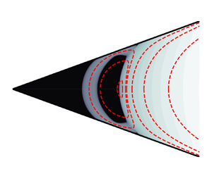
Figure 2. Schematic of viscoplastic eddies in a wedge. Black regions represent unyielded fluid, and only half of the domain is shown, with the lower half determined by anti-symmetry under vertical reflection. No eddies are present in region (a), where the fluid is unyielded, and the eddies in region (b) are essentially unchanged from the corresponding viscous eddies described by Moffatt (Reference Moffatt1964).
In the following numerical simulations we will sometimes take a value of  $\textit {Bi}\ll 1$, at which new eddies open up below the one at
  $r=1$. These cases are included to demonstrate the self-similarity between two consecutive generations of eddies, and to explore the critical point at which a new eddy is formed; however, we point out that when the problem is scaled as detailed above, then these Bingham numbers are technically inadmissable. Formally, due to the infinite, self-similar domain and the self-similar nature of the Moffatt solution being applied as a boundary condition, these cases should be considered as identical to rescaled problems in which the lengths are divided by
  $S_0$, velocities by
  $S_1$ and the Bingham number by
  $S_2$. And, after such a rescaling, they would be consistent with the scaled problem defined above, with
  $\textit {Bi}=O(1)$ and the smallest eddy occurring just below
  $r=1$.
After non-dimensionalisation, the governing equations for velocity,  $\boldsymbol {u}=(u_r,u_\theta )$, pressure,
  $p$, and deviatoric stress,
  $\boldsymbol {\tau }$, are
 $$\begin{gather} \boldsymbol{\nabla}\boldsymbol{\cdot}\boldsymbol{u}=0, \end{gather}$$
 $$\begin{gather}\boldsymbol{\nabla} p=\boldsymbol{\nabla}\boldsymbol{\cdot}\boldsymbol{\tau}, \end{gather}$$
representing incompressibility and the balance of momentum. The Bingham constitutive law is given in non-dimensional form by
 \begin{equation} \boldsymbol{\tau}=\left(1+\frac{\textit{Bi}}{\left\|\dot{\boldsymbol{\gamma}}\right\|}\right)\dot{\boldsymbol{\gamma}} \ \text{when}\ \left\|\boldsymbol{\tau}\right\|>\textit{Bi}, \quad \dot{\boldsymbol{\gamma}}=0 \ \text{otherwise.} \end{equation}
We consider anti-symmetric solutions in the upper half of the domain,  $0\leqslant \theta \leqslant \alpha$, with boundary conditions
 $$\begin{gather} \boldsymbol{u}=0 \quad \text{on}\ \theta=\alpha, \end{gather}$$
 $$\begin{gather}u_r=0 \quad \text{on } \theta=0, \end{gather}$$
 $$\begin{gather}(u_r,u_\theta)\sim \left(\frac{1}{r}\frac{\partial \psi_V}{\partial \theta}, -\frac{\partial \psi_V}{\partial r}\right) \quad \text{as } r\to\infty, \end{gather}$$
representing no-slip, anti-symmetry and the far-field condition, respectively.
3. Numerical method
We compute finite element numerical simulations, using the augmented-Lagrangian method (for full details see, e.g. Saramito Reference Saramito2016), over a wide range of  $\textit {Bi}$ and for
  $\alpha =5^{\circ }, 20^{\circ }, 45^{\circ }$ and
  $60^{\circ }$ (as well as
  $\alpha =0^{\circ }$ in Appendix B). This algorithm circumvents the singular nature of the constitutive law at the yield surfaces via the introduction of an independent tensorial field,
  $\boldsymbol{\mathsf{D}}$, representing the strain-rate tensor, and a Lagrangian multiplier, standing for the deviatoric stress tensor, which enforces the equivalence of
  $\boldsymbol{\mathsf{D}}$ and
  $\dot {\boldsymbol {\gamma }}(\boldsymbol {u})$. In contrast to regularisation methods, in which unyielded regions are replaced with regions of very high viscosity, the augmented-Lagrangian method accurately represents solid regions by setting
  $\boldsymbol{\mathsf{D}}=\boldsymbol {0}$ for stresses below the yield stress. We implement the numerical method in FEniCS, a numerical implementation of the finite element method (Logg, Mardal & Wells Reference Logg, Mardal and Wells2012; Alnæs et al. Reference Alnæs, Blechta, Hake, Johansson, Kehlet, Logg, Richardson, Ring, Rognes and Wells2015) and employ a simple adaptive mesh refinement algorithm where periodically in the augmented-Lagrangian iterations (typically every 50 iterations) we refine cells in the vicinity of the yield surface. Specifically, we refine cells for which the deviatoric stress variable lies within some tolerance of
  $Bi$. For the first refinement, we use a tolerance
  $Bi/2$, and decrease the tolerance by
  $25\,\%$ for each subsequent refinement to encompass consistently the yield surface while somewhat limiting the number of new cells produced. We stop refining after five refinement steps, or once the new mesh size would be above some chosen limit – in this case, 280 000 cells. In place of the far-field boundary condition, (2.12), we truncate the domain at the straight boundary
  $x=r\cos \theta =x_R$ and impose the viscous Moffatt (Reference Moffatt1964) solution
 \begin{equation} (u_r,u_\theta)= \left(\frac{1}{r}\frac{\partial \psi_V}{\partial \theta}, -\frac{\partial \psi_V}{\partial r}\right) \end{equation}
on this boundary. When choosing the truncation position,  $x_R$, we require that the strain rate is significantly larger than
  $\textit {Bi}$ along
  $x=x_R$, so that the viscous solution is a good approximation to the viscoplastic solution at the truncated boundary and, hence, that the solution is essentially unchanged by the truncation of the domain. In particular this requires avoiding any of the points at which the strain rate vanishes in the Moffatt (Reference Moffatt1964) solution. To check the impact of truncation at
  $x=x_R$, simulations were repeated on domains at least
  $50\,\%$ larger and the velocity solution and inner plug depths,
  $d$, were found to differ by less than
  $1\,\%$ for all solutions. The values of
  $x_R$ varied between
  $1.5$ and
  $15$ for the different values of
  $\textit {Bi}$ and
  $\alpha$, with the largest domain being needed for the simulation with
  $\alpha =60$ and
  $\textit {Bi}=2$. All simulations converged to a residual,
  $\|\sqrt {({\mathsf{D}}_{ij}-\dot {\gamma }_{ij})({\mathsf{D}}_{ij}-\dot {\gamma }_{ij})}\|_{L^{2}}$, of less than
  $10^{-5}$, with many of the smaller Bingham number simulations converging to significantly lower residuals.
4. Results and key scalings
A typical set of numerical solutions is given in figure 3 demonstrating the existence of three unyielded regions, as observed in Roustaei & Frigaard (Reference Roustaei and Frigaard2013): a static unyielded region in the corner of the wedge; a small static unyielded region on the boundary at the stagnation point between eddies; and a plug region in solid-body motion within the eddy. All regions decrease in size as  $\textit {Bi}$ decreases, until a new eddy forms at sufficiently small
  $\textit {Bi}$. While Abbott et al. (Reference Abbott, Braun, Breward, Cook, Cromer, Edwards, Hibdon, Please, Taroni and Zhang2009) predicted an approximately circular plug rotating at the ‘centre’ of the eddy, we note that this plug is somewhat unintuitive, not encompassing the centre of the eddy and, as a result, being closer to a semi-circle in shape. This is due to the fact that in Moffatt eddies, the point on the wedge's symmetry axis at which the strain rate vanishes is distinct from the point where the velocity vanishes. Furthermore, though this plug is undergoing solid-body rotation, there is no requirement that its boundary is circular, since the yield surface need not be a material surface (streamlines can exit and enter the plug as the fluid element yields and unyields). We see that the flow in the eddy in
  $r>1$ is largely unchanged for these Bingham numbers, although the streamlines are slightly altered at the inner extent of the eddy for larger
  $\textit {Bi}$, and that once a new eddy has formed, the unyielded regions in the eddy above have become negligibly small, as anticipated. Note also that, as discussed in § 2, the solution in panel (d) is equivalent to a rescaled problem where the first eddy has its rightmost extent at
  $r=1$ and
  $Bi$ is multiplied by
  $S_2^{-1}=\exp ({(\lambda _r-2){\rm \pi} /\lambda _i})\approx 170$. This gives
  $Bi=3.0$ (to
  $2$ significant figures), and so we expect panels
  $(a)$ and
  $(d)$ to be equivalent up to scaling, as is observed.

Figure 3. Contours of the modulus of the strain rate,  $\|\dot {\boldsymbol {\gamma }}\|$, (grey scale) and streamlines (red) for
  $\alpha =20^{\circ }$ and (a)
  $Bi=3$, (b)
  $Bi=1$, (c)
  $Bi=0.25$ and (d)
  $Bi=0.018$. The unyielded regions are shown in black. The critical Bingham number at which a new eddy forms,
  $\textit {Bi}_c$, lies somewhere between the value of
  $\textit {Bi}$ for panels (c) and (d). Note the logarithmic scale for the strain rate.
Two key features of the problem are the extent of the stagnant unyielded plug in the corner as a function of  $Bi$, and the critical Bingham numbers,
  $Bi_c$, at which a new eddy forms. We measure the former as the distance,
  $d$, of the yield surface from the vertex of the wedge, along the
  $\theta =0$ plane. The stars in figure 4 show
  $d$ against
  $Bi$ for four values of
  $\alpha$, determined from the numerical simulations. The first plot shows how
  $d$ decreases with
  $Bi$ after the creation of the second eddy and before the creation of a third, while the log–log plots demonstrate the existence and location of the critical Bingham numbers at which the value of
  $d$ jumps due to the formation/disappearance of an eddy, and the equivalence up to scaling of consecutive eddies evidenced by the translational periodicity of the curves. In the following section we provide a heuristic argument for approximating
  $Bi_c$ and the values of
  $d$ before and after a new eddy forms.

Figure 4. Extent of the static plug in the corner of the wedge,  $d$, as a function of
  $Bi$. Symbols show numerical results while the dotted lines show our heuristic predictions. (a) Plots of
  $\alpha =20^{\circ }$ on a linear-linear scale, showing variation of
  $d$ with
  $Bi$. Log–log plots across a larger range of
  $Bi$ are given for (b)
  $\alpha =5^{\circ }$, (c)
  $\alpha =20^{\circ }$, (d)
  $\alpha =45^{\circ }$ and (e)
  $\alpha =60^{\circ }$, showing the jumps at critical values of
  $Bi$ where a new eddy forms and the self-similarity of consecutive generations of eddies. The red points
  $A$,
$A$,  $B$,
$B$,  $C$ and
  $D$ in panel (c) indicate the four points derived in the heuristic approximation, as detailed in § 4.1.
4.1. The critical Bingham number
A heuristic argument to approximate the critical Bingham number,  $Bi_c$, for a given half-angle,
  $\alpha$, is as follows. We observe that the eddy adjacent to a newly opened eddy fully contains the corresponding viscous Moffatt (Reference Moffatt1964) eddy and consider a semi-circle, meeting the boundary tangentially, with diameter centred on
  $(x_0,0)$, where
  $x_0$ is the smallest
  $x$-coordinate attained by this Moffatt eddy (see figure 5). Note that
  $x_0$ is known a priori, since the Moffatt solution is known analytically, but is only a heuristic approximation to the minimum distance attained by the viscoplastic eddy. Appendix A outlines a more rigorous approach to determine the region of the static corner plug that yields to rotation as the Bingham number is reduced; however, for the purposes of a heuristic argument, we appeal to the observation from numerical simulations that this semi-circle is a good approximation to the true yield surface, as seen in figure 5. The normal stresses acting on the diameter of the semi-circle exert a dimensionless torque, denoted by
  $2G$, around
  $(x_0,0)$ on the fluid contained in the semi-circle, which must be balanced by the torque due to the tangential stresses along the circumference of the semi-circle (since, in the absence of inertia, torques must balance). The dimensionless torque,
  $G$, is given by
 \begin{equation} G=\left\lvert\int_0^{R} y\left({-}p+\tau_{xx}\right){{\rm d}y}\right\rvert,\end{equation}
where  $R=x_0\sin \alpha$ is the radius of the semi-circle, and the integral is calculated along
  $x=x_0$. While the fluid is unyielded along the circular arc, the maximum possible torque per unit length is
  $R\textit {Bi}$. In practice, the semi-circle may extend slightly beyond the yield surface (see figure 5) which would slightly alter the torque along the arc in this region but nonetheless the maximum torque along the circumference in the upper half of the wedge is approximately
  ${\rm \pi} R^{2}\textit {Bi}/2$. At the critical Bingham number,
  $\textit {Bi}_c$, we hence have
 \begin{equation} \frac{{\rm \pi} R^{2}\textit{Bi}_c}{2}\approx G.\end{equation}
The final approximation we make is to use the purely viscous solution for  $p$ and
  $\tau _{xx}$, encoded by the streamfunction
  $\psi _V$, (2.5), in (4.1), when evaluating
  $G$ in (4.2). This allows us to calculate an approximation for
  $\textit {Bi}_c$ for any
  $\alpha$, purely from the Moffatt solution given by (2.5). Figure 6(a) shows the value of
  $G$ calculated using the Moffatt solution, while the stars are from the numerical simulations shown in figure 5(a–d). The close correspondence of these curves demonstrates the validity of the approximation. Figure 6(b) shows the predicted value of
  $\textit {Bi}_c$ as a function of
  $\alpha$, alongside the smallest Bingham numbers of numerical simulations at which the new eddy had not yet formed (representing a numerical upper bound for
  $\textit {Bi}_c$). Interestingly, the predicted value of
  $\textit {Bi}_c$ is approximately constant over a wide range of angles,
  $15^{\circ }\lessapprox \alpha \lessapprox 45^{\circ }$, diverging like
  $1/\alpha$ as
  $\alpha \to 0$ and tending to
  $0$ as
  $\alpha \to \alpha _c$. The latter is anticipated since the relative intensity of consecutive eddies vanishes in this limit requiring a vanishing Bingham number to exhibit additional eddies. The divergent behaviour as
  $\alpha \to 0$ can also be understood, by instead considering
  $\alpha \to 0$ with
  $r\alpha =1$ fixed, which is the typical way to treat this limit and which represents convergence to a uniform channel of width 2, for
  $\alpha$ in radians. We previously scaled lengths by
  $L_0$ to set the eddy of interest to
  $r=1$, so to scale this eddy instead to
  $r=1/\alpha$ requires a length scale of
  $\tilde {L}=\alpha L_0$, giving a new Bingham number
 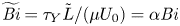 $\widetilde {\textit {Bi}}=\tau _Y \tilde {L}/(\mu U_0)=\alpha \textit {Bi}$. We anticipate that the corresponding scaled critical Bingham number,
  $\widetilde {\textit {Bi}}_c=\alpha \textit {Bi}_c$, is finite in the controlled limit, representing the Bingham number at which a new eddy forms between parallel plates, and from the heuristic calculation above, we find that
 \begin{equation} \lim_{\alpha\to 0}\widetilde{\textit{Bi}}_c=\lim_{\alpha\to 0}\alpha\textit{Bi}_c= 0.0022\ \text{(to 2 significant figures)}, \end{equation}
is the critical Bingham number for this limit. In fact this limit can be tackled directly by considering the eddy flow between parallel plates, as is demonstrated in Appendix B.

Figure 5. Examples of solutions before (a–d) and after (e–h) a new eddy has formed. The dotted line shows the dividing streamline  $\psi _V=0$ from the corresponding Moffatt solutions while the red lines show the semi-circles considered in § 4.1.

Figure 6. (a) Torque,  $G$, acting on the vertical radius of the semi-circle considered in § 4.1 using the corresponding Moffatt solution (dotted) and from the viscoplastic numerical simulations shown in the top row of figure 5 (stars), as a function of the wedge half-angle,
  $\alpha$. (b) The corresponding critical Bingham number,
  $\textit {Bi}_c$, calculated from (4.2) (solid line), as a function of the wedge half-angle,
  $\alpha$. The red dotted line shows the divergent behaviour as
  $\alpha \to 0$, given by
  $\textit {Bi}_c\sim 0.0022/\alpha$, while the stars indicate the smallest Bingham numbers of numerical simulations in which the new eddy has not yet opened up (and, hence, represent numerical upper bounds for
  $\textit {Bi}_c$).
Using  $x_0$,
  $R$ and
  $\textit {Bi}_c$ we can also give a heuristic approximation for the extent,
  $d$, of the static plug in the corner of the wedge, measured along the
  $\theta =0$ plane, as a function of
  $\textit {Bi}$. We have
  $d\approx x_0$ as
  $\textit {Bi}\to \textit {Bi}_c$ from above, and
  $d\approx x_0-R=x_0(1-\sin \alpha )$ as
  $\textit {Bi}\to \textit {Bi}_c$ from below. We can then use self-similarity with the scale factors given in § 2 to scale up/down to the values of
  $d$ and
  $\textit {Bi}$ at the start of the eddy further from/nearer to the vertex. Specifically, this gives four points on the
  $\textit {Bi}-d$ curve:
 \begin{equation}
\left.\begin{gathered} A=\left(\textit{Bi}_c, x_0(1-\sin\alpha)\right),\quad B= \left(\textit{Bi}_c, x_0\right), \\
C=\left(\exp({\left(\lambda_r-2\right){\rm \pi}/\lambda_i})\textit{Bi}_c, \exp({{\rm \pi}/\lambda_i})x_0(1-\sin\alpha)\right), \\
\qquad D= \left(\exp({\left(\lambda_r-2\right){\rm \pi}/\lambda_i}) \textit{Bi}_c, \exp({{\rm \pi}/\lambda_i})x_0\right) , \end{gathered}\right\}
\end{equation}
\begin{equation}
\left.\begin{gathered} A=\left(\textit{Bi}_c, x_0(1-\sin\alpha)\right),\quad B= \left(\textit{Bi}_c, x_0\right), \\
C=\left(\exp({\left(\lambda_r-2\right){\rm \pi}/\lambda_i})\textit{Bi}_c, \exp({{\rm \pi}/\lambda_i})x_0(1-\sin\alpha)\right), \\
\qquad D= \left(\exp({\left(\lambda_r-2\right){\rm \pi}/\lambda_i}) \textit{Bi}_c, \exp({{\rm \pi}/\lambda_i})x_0\right) , \end{gathered}\right\}
\end{equation}
where  $A$ to
  $B$ and
  $C$ to
  $D$ are vertical jumps occurring at the formation/disappearance of an eddy, while between
  $B$ and
  $C$,
$C$,  $d$ is a continuous, increasing function of
  $\textit {Bi}$. The form of this function is shown, from numerical solutions for
  $\alpha =20^{\circ }$, in figure 4a), but for the purposes of a simple approximation, linear interpolation can be used between points
  $B$ and
  $C$. Figure 4 shows good agreement between this heuristic approximation and the numerical simulations, despite its simplicity.
4.2. Flow fields when  $0<\textit {Bi}_c-\textit {Bi}\ll 1$
Slightly below the yield stress at which a new eddy forms, a thin layer of yielded fluid separates the static corner plug from the rotating semi-circular plug, meaning we can employ a boundary layer analysis similar to those detailed by Balmforth et al. (Reference Balmforth, Craster, Hewitt, Hormozi and Maleki2017), Hewitt & Balmforth (Reference Hewitt and Balmforth2018) and Taylor-West & Hogg (Reference Taylor-West and Hogg2021). This boundary layer analysis will determine the scalings of the width of the yielded layer and the rotation rate of the rotating plug, with the difference between the Bingham number and  $Bi_c$. In fact there are two distinct boundary layer scalings with one applying between the rotating plug and the rigid boundary and another between the static and rotating plugs. The former is asymptotically thinner than the latter; in the former, the viscous shear stresses provide the leading-order contribution to the torque balance on the rotating plug, whereas in the latter, plastic stresses are non-negligible.
Figure 7 shows a schematic of the boundary layer geometry. The governing small parameter is  $\Delta \textit {Bi}=\textit {Bi}_c-\textit {Bi}$, which we refer to as the Bingham number deficit, and there are a number of quantities that scale with this quantity: the boundary layer thickness between the wall and the rotating plug,
  $\epsilon _1$; the boundary layer thickness between the rotating plug and stagnant corner plug,
  $\epsilon _2$; and the rotation rate of the rotating plug,
  $\varOmega$. Note there is also a short section of wider boundary layer after the narrow section where the boundary layer meets the adjacent eddy. The width here is also
  $O(\epsilon _2)$ but we will neglect this section for the clarity of the following discussion, appealing to the shortness of the region to justify this decision. The direction of rotation depends on which eddy is being considered, but we will assume clockwise rotation, as relevant to the first new eddy to form as
  $\textit {Bi}$ is decreased as in figure 2. Following the construction of Balmforth et al. (Reference Balmforth, Craster, Hewitt, Hormozi and Maleki2017), we take curvilinear coordinates,
  $(s,n)$, and velocities,
  $(u_s,u_n)$, along and across the boundary layer (although we note that polar coordinates would also be an appropriate choice here), where
  $s=0$ at the axis of symmetry of the wedge. The full system of equations are then (see, e.g. Balmforth et al. Reference Balmforth, Craster, Hewitt, Hormozi and Maleki2017)
 $$\begin{gather} \frac{\partial u_s}{\partial s}+\left(1-\kappa n\right)\frac{\partial u_n}{\partial n}-\kappa u_n=0, \end{gather}$$
 $$\begin{gather}\frac{\partial \tau_{ss}}{\partial s}+\left(1-\kappa n\right)\frac{\partial \tau_{sn}}{\partial n}-2\kappa\tau_{sn}=\frac{\partial p}{\partial s}, \end{gather}$$
 $$\begin{gather}\frac{\partial \tau_{sn}}{\partial s}+\left(1-\kappa n\right)\frac{\partial \tau_{nn}}{\partial n}+\kappa\left(\tau_{ss}-\tau_{nn}\right)=\frac{\partial p}{\partial n}, \end{gather}$$
where  $\kappa$ is the curvature of the boundary layer. For an approximately circular boundary layer, we have
  $\kappa \approx -{1}/{R}$ (with the sign determined from the orientation of the coordinate axes).

Figure 7. Schematic of boundary layer geometry shortly after a new eddy has formed. The grey regions are unyielded fluid, and the central plug is in clockwise solid-body rotation around the point  $O$ with rotation rate
  $\varOmega$.
The components of strain rate and deviatoric stress are given by
 $$\begin{gather} \dot{\gamma}_{ss}={-}\dot{\gamma}_{nn}=\frac{2}{1-\kappa n}\left(\frac{\partial u_s}{\partial s}-\kappa u_n\right), \quad \dot{\gamma}_{sn}=\frac{1}{1-\kappa n}\left(\frac{\partial u_n}{\partial s}+\kappa u_s\right)+\frac{\partial u_s}{\partial n}, \end{gather}$$
 $$\begin{gather}\begin{pmatrix} \tau_{ss} \\ \tau_{sn} \end{pmatrix}=\left(1+\frac{\textit{Bi}}{\left\|\dot{\boldsymbol{\gamma}}\right\|}\right)\begin{pmatrix} \dot{\gamma}_{ss} \\ \dot{\gamma}_{sn} \end{pmatrix} \quad \text{when } \left\|\boldsymbol{\tau}\right\|>\textit{Bi}, \ \text{and } \dot{\boldsymbol{\gamma}}=\boldsymbol{0} \quad \text{otherwise.} \end{gather}$$
In each of the boundary layer regions,  $j=1$ and
  $2$, we define scaled coordinates and velocities by
 \begin{equation} (s,n)=(s,\epsilon_j\eta_j), \quad (u_s,u_n)=R\varOmega(U_s,\epsilon_j U_n) \quad \text{for } j=1,2, \end{equation}
where  $u_s$ is scaled by the velocity of the rotating yield surface, and
  $u_n$ is scaled accordingly from the conservation of mass, (4.5). Retaining only potentially leading-order terms we find that
 $$\begin{gather} \tau_{sn}={-}\textit{Bi}+\frac{R\varOmega}{\epsilon_j}\frac{\partial U_s}{\partial \eta_j}+2\epsilon_j^{2}\textit{Bi}\left(\frac{\partial U_s}{\partial s}\right)^{2}\left(\frac{\partial U_s}{\partial \eta_j}\right)^{{-}2}+\dots, \end{gather}$$
 $$\begin{gather}\tau_{ss}={-}2\epsilon_j\textit{Bi}\left(\frac{\partial U_s}{\partial s}\right)\left(\frac{\partial U_s}{\partial \eta_j}\right)^{{-}1}+\dots, \end{gather}$$
where the sign of the first term on the right-hand side of (4.11) is due to the clockwise rotation of the rotating plug and we note that  $R$ and
  $Bi$ are
  $O(1)$ as
  $\Delta \textit {Bi}\to 0$. To account for the curvature term in (4.6), we write the pressure in each region as
 \begin{equation} p={-}\frac{2\textit{Bi}}{R}s+\frac{R\varOmega}{\epsilon_j^{2}}P(s,\eta_j)+\dots.\end{equation}
With this substitution we find that, to leading order, (4.6) and (4.7) are given by
 $$\begin{gather}
\frac{\partial P}{\partial s}\!=\!\frac{\partial^{2} U_s}{\partial \eta_j^{2}}\!+\!2\frac{\epsilon_j^{3}\textit{Bi}}{R\varOmega} \frac{\partial}{\partial\eta_j}\left(\left(\frac{\partial
U_s}{\partial s}\right)^{2}\left(\frac{\partial U_s} {\partial \eta_j}\right)^{{-}2}\right) \!-\!2\frac{\textit{Bi}\epsilon_j^{3}}{R\varOmega}\frac{\partial}{\partial
s}\left(\left(\frac{\partial U_s}{\partial
s}\right)\left(\frac{\partial U_s}{\partial
\eta_j}\right)^{{-}1}\right)+\dots,
\end{gather}$$
$$\begin{gather}
\frac{\partial P}{\partial s}\!=\!\frac{\partial^{2} U_s}{\partial \eta_j^{2}}\!+\!2\frac{\epsilon_j^{3}\textit{Bi}}{R\varOmega} \frac{\partial}{\partial\eta_j}\left(\left(\frac{\partial
U_s}{\partial s}\right)^{2}\left(\frac{\partial U_s} {\partial \eta_j}\right)^{{-}2}\right) \!-\!2\frac{\textit{Bi}\epsilon_j^{3}}{R\varOmega}\frac{\partial}{\partial
s}\left(\left(\frac{\partial U_s}{\partial
s}\right)\left(\frac{\partial U_s}{\partial
\eta_j}\right)^{{-}1}\right)+\dots,
\end{gather}$$ $$\begin{gather}\frac{\partial P}{\partial \eta_j}=2\frac{\textit{Bi}\epsilon_j^{3}}{R\varOmega}\frac{\partial}{\partial\eta_j}\left(\left(\frac{\partial U_s}{\partial s}\right)\left(\frac{\partial U_s}{\partial \eta_j}\right)^{{-}1}\right)+\dots. \end{gather}$$
There are now two possible regimes in which viscous terms enter the momentum balance. Assuming  $\epsilon _j^{3}/\varOmega \ll 1$, we have
  $\partial P/\partial \eta _j=0$ to leading order and
 \begin{equation} \frac{\textrm{d} P}{\textrm{d} s}=\frac{\partial^{2} U_s}{\partial \eta_j^{2}}\end{equation}
giving a quadratic profile for  $U_s$. This situation applies for
  $j=1$, where one side of the boundary layer is bounded by a rigid wall, but impossible for
  $j=2$ since the strain rate
  $\partial U_s/\partial \eta _2$ must vanish at two distinct points, namely at both sides of the boundary layer, where it meets unyielded fluid. Hence, in the thinner region of the boundary layer we have
  $\epsilon _1^{3}/\varOmega \ll 1$, with the exact scaling undetermined until later, while in the wider region we have
 \begin{equation} \epsilon_2^{3}\textit{Bi}/(R\varOmega)=1 \implies \epsilon_2=O(\varOmega^{1/3}), \end{equation}
and a boundary layer solution governed by the partial differential equation derived by Oldroyd (Reference Oldroyd1947)
 \begin{equation} \frac{\partial}{\partial\eta_2}\left(\frac{\partial U_s}{\partial \eta_2}+2\left(\frac{\partial U_s}{\partial s}\right)^{2}\left(\frac{\partial U_s}{\partial \eta_2}\right)^{{-}2}\right)-4\frac{\partial}{\partial s}\left(\left(\frac{\partial U_s}{\partial s}\right)\left(\frac{\partial U_s}{\partial \eta_2}\right)^{{-}1}\right)=F(s)\end{equation}
for some function of integration,  $F(s)$. In both sections of the boundary layer (
 $\,j=1,2$) we have boundary conditions
 \begin{equation} U_s=0 \text{ at } \eta_j=\eta_j^{+} \quad\text{and}\quad U_s=1,\quad \frac{\partial U_s}{\partial \eta_j}=0\ \text{at}\ \eta_j=\eta_j^{-}, \end{equation}
where  $\eta _j^{+}$ and
  $\eta _j^{-}$ are the limits of the boundary layer, and in the wider section of the boundary layer, where the layer is sandwiched between regions of unyielded fluid, we have the additional boundary condition
 \begin{equation} \frac{\partial U_s}{\partial \eta_2}=0\quad \text{at}\ \eta_2=\eta_2^{+}. \end{equation}
In the thinner region of the boundary layer, we integrate (4.16) and apply the boundary conditions to find
 \begin{equation} U_s=\frac{1}{2}\frac{\textrm{d}P}{\textrm{d}s}\left(\left(\eta_1^{+}-\eta_1\right)^{2}-2\left(\eta_1^{+}-\eta_1^{-}\right)\left(\eta_1^{+}-\eta_1\right)\right), \quad \frac{\textrm{d}P}{\textrm{d}s}={-}\frac{2}{\left(\eta_1^{+}-\eta_1^{-}\right)^{2}}. \end{equation}
Conservation of mass imposes an additional constraint
 \begin{equation} \frac{\textrm{d}}{\textrm{d}s}\int_{\eta_1^{-}}^{\eta_1^{+}}U_s\,\textrm{d}\eta={-}\frac{\textrm{d}\eta_1^{-}}{\textrm{d}s}, \end{equation}
representing the fact that divergence of the flux must be accounted for by flow through the boundaries of the boundary layer. This gives  $\eta _1^{-}$ in terms of
  $\eta _1^{+}$ as
 \begin{equation} \eta_1^{-}={-}(2\eta_1^{+}+W_0), \end{equation}
where  $W_0$ is a constant of integration and is
  $O(1)$. Since
  $\eta _1^{+}$ is given by the fixed position of the wall, it is a known function of
  $s$. In the vicinity of the point at which the semi-circle meets the rigid boundary,
  $s\approx s_0=R({\rm \pi} /2-\alpha )$, we have
 \begin{equation} \eta_1^{+}=\frac{(s-s_0)^{2}}{2\epsilon_1 R} \quad\text{and}\quad \eta_1^{+}-\eta_1^{-}=W_0+\frac{3(s-s_0)^{2}}{2\epsilon_1 R}, \end{equation}
to leading order. Thus, we interpret  $W_0$ as the width of the boundary layer at
  $s=s_0$, in boundary layer coordinates.
Since the pressure vanishes at the wedge's axis of symmetry by anti-symmetry, the total pressure change along the boundary layers is  $O(1)$, given by the pressure at the point where the boundary layer meets the adjacent eddy – and here the solution remains unchanged to leading order by small changes in the Bingham number,
  $\Delta \textit {Bi}$. The contribution to the pressure gradient along the boundary layer,
  $\partial p/\partial s$, due to the curvature of the boundary layer is
  $-2\textit {Bi}/R=O(1)$. This is the leading-order contribution in the wider sections of the boundary layer, and contributes a total pressure drop of
  $-{\rm \pi} \textit {Bi}$ over the length of the boundary layer. In general this does not match the pressure where the boundary layer meets the fully yielded adjacent eddy (see, e.g. figure 8b) and, thus, we require an additional
  $O(1)$ pressure jump along the thinner section of the boundary layer. This is only possible if the dominant contribution to the pressure gradient,
  $\partial p/\partial s$, in the thinner section of the boundary layer is due to the second term in (4.13). Substituting for
  $\eta _1^{+}$ we find that
 \begin{equation} \frac{\textrm{d}P}{\textrm{d}s}={-}\frac{2}{\left(W_0+\dfrac{3\left(s-s_0\right)^{2}} {2\epsilon_1R}\right)^{2}},\end{equation}
which is  $O(1)$ over the region where
  $s-s_0=O(\sqrt {\epsilon _1})$, and decays outside this region. Hence, the total pressure drop over the thinner region is
 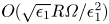 $O(\sqrt {\epsilon _1}R\varOmega /\epsilon _1^{2})$. In fact, we can integrate (4.25) analytically to obtain the leading-order pressure drop over the thinner region as
 \begin{equation} \frac{R\varOmega}{\epsilon_1^{2}}\int_{-\infty}^{\infty}\frac{\textrm{d}P} {\textrm{d}s}\textrm{d}s=\sqrt{\frac{2}{3}}{\rm \pi}\frac{R^{3/2}\varOmega} {\left(\epsilon_1W_0\right){}^{3/2}}. \end{equation}
In either case, we conclude that
 \begin{equation} \epsilon_1=O(\varOmega^{2/3})=O(\epsilon_2^{2}).\end{equation}
Figure 8. (a) Rotation rate  $\varOmega$ as a function of
  $\textit {Bi}$ for
  $\alpha =20^{\circ }$, measured in numerical simulations (stars) and the scaling relationship
 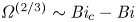 $\varOmega ^{(2/3)}\sim \textit {Bi}_c-\textit {Bi}$. The horizontal dashed line shows
  $\varOmega _V^{(2/3)}$, where
  $\varOmega _V$ is the rotation rate at the point where the strain rate vanishes in the viscous solution. (b) Pressure,
  $p$, as a function of the coordinate along the boundary layer,
  $s$, for three values of the Bingham number deficit,
  $\Delta \textit {Bi}$, indicated in the legend. The black dotted line shows the constant gradient
  $-2\textit {Bi}_c/R$ predicted in the thicker section of the boundary layer for small
  $\Delta \textit {Bi}$, and the vertical grey dashed line marks the narrowest point of the boundary layer.
Finally, we consider the additional torque along the circular arc, above that provided by the yield stress, given by
 \begin{equation} -\int_0^{{R{\rm \pi}}/{2}} R(\tau_{sn}+\textit{Bi})\,{\rm d}s=G(\textit{Bi})-\frac{{\rm \pi} R^{2}\textit{Bi}}{2},\end{equation}
where  $G(\textit {Bi})$ again represents the torque acting on the upper half of the diameter of the semi-circle due to normal stresses in the yielded flow to the right of the plug (see (4.1)), and is substituted for
  $-\int _0^{R{\rm \pi} /2}R\tau _{sn}\,\textrm {d}s$ by torque balance. Since this diameter lies primarily in the adjacent eddy, in which the solution varies smoothly with
  $\textit {Bi}$, we can use a Taylor series to write
 \begin{equation} G(\textit{Bi})=G(\textit{Bi}_c)+O(\textit{Bi}_c-\textit{Bi})=\frac{{\rm \pi} R^{2} \textit{Bi}_c}{2}+O(\Delta\textit{Bi}), \end{equation}
and, thus,
 \begin{equation} -\int_0^{{R{\rm \pi}}/{2}} R(\tau_{sn}+\textit{Bi})\,{\rm d}s=O(\Delta\textit{Bi}). \end{equation}
Substituting for  $\tau _{sn}$ from (4.11), and using (4.17), the contributions to this additional torque from region 2 is
 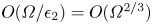 $O(\varOmega /\epsilon _2)=O(\varOmega ^{2/3})$. In region 1, similarly to the pressure gradient, the viscous shear stress is dominated by a region of length
  $O(\sqrt {\epsilon _1})$ where
  $\partial U_s/\partial \eta _1=O(1)$. And hence, using (4.11) and (4.27), the additional torque from region 1 is
  $O(\sqrt {\epsilon _1}\varOmega /\epsilon _1)=O(\varOmega ^{2/3})$, as for region 2. Thus,
  $\Delta \textit {Bi}\sim \varOmega ^{2/3}$, and we obtain the scalings
 \begin{equation} \varOmega\sim\Delta\textit{Bi}^{3/2}, \quad \epsilon_2\sim\Delta\textit{Bi}^{1/2} \quad \text{and}\quad \epsilon_1\sim\Delta\textit{Bi}. \end{equation}
Figure 8 provides evidence for the validity of this boundary layer theory, from a sequence of numerical simulations for  $\alpha =20^{\circ }$. We measure
  $\varOmega$ as the rotation rate at the point on the wedge's symmetry axis at which the strain rate vanishes in the corresponding Moffatt (Reference Moffatt1964) solution. This point is always inside the central rotating plug in the viscoplastic solutions. The left panel shows how
  $\varOmega \sim \Delta \textit {Bi}^{3/2}$ when
  $\textit {Bi}\to \textit {Bi}_c$ from below, and rises up to the rotation rate,
  $\varOmega _V$, from the viscous, Moffatt solution, as
  $\textit {Bi}$ decreases. The right panel shows how pressure varies along the boundary layer, for three values of the Bingham number deficit,
  $\Delta \textit {Bi}$, verifying that the pressure gradient approaches the constant
  $-2\textit {Bi}_c/R$ in the first, wider, part of the boundary layer, before becoming large in a short section of the layer, resulting in an
  $O(1)$ overall pressure change, essentially independent of
  $\Delta \textit {Bi}$.
In region 2 we can solve (4.18) by means of a similarity solution detailed by Balmforth et al. (Reference Balmforth, Craster, Hewitt, Hormozi and Maleki2017) and find that
 \begin{equation} U_s=\frac{1}{2}+\frac{1}{4}\zeta\left(\zeta^{2}-3\right), \quad \zeta={-}\frac{\eta_2-\eta_2^{m}}{Y(s)}, \end{equation}
where  $\eta _2^{m}=(\eta _2^{+}+\eta _2^{-})/2$ is the mid-line of the boundary layer and
  $Y(s)=(\eta _2^{+}-\eta _2^{-})/2$ is its half-width, given implicitly by
 \begin{equation} Y_E^{3/2}\left(\tan^{{-}1}\sqrt{\frac{Y/Y_E}{1-Y/Y_E}}-\sqrt{\frac{Y}{Y_E} \left(1-\frac{Y}{Y_E}\right)}\right)=\frac{\sqrt{3}}{2}\left(\tilde{s}_0-s\right). \end{equation}
Here  $s=\tilde {s}_0$ is the apparent origin of the similarity solution, at which location
  $Y(\tilde {s}_0)=0$, and
 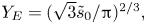 $Y_E=(\sqrt {3}\tilde {s}_0/{\rm \pi} )^{2/3},$ is the maximum half-width of the boundary layer. Asymptotically, to leading order this section of the boundary layer must end at
 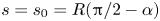 $s=s_0=R({\rm \pi} /2-\alpha )$ with vanishing width, and, hence, to leading order we must have
  $\tilde {s}_0=s_0$. The complete leading-order boundary layer solution would then be obtained by fixing the constants
  $W_0$ and
  $\varOmega _0$, where
  $\varOmega \sim \varOmega _0\Delta \textit {Bi}^{3/2}$, by enforcing both the pressure drop over region 1 and the torque over the entire boundary layer. This calculation requires additional detailed analysis of the fully yielded flow within the eddy adjacent to the boundary layers and is not attempted here. Instead, the boundary layer structure has revealed the asymptotic scalings of
  $\epsilon _1$,
  $\epsilon _2$ and
  $\varOmega$ upon the Bingham number deficit,
  $\Delta \textit {Bi}$.
The predictions of boundary layer shape can also be compared with numerics by directly measuring the empirical rotation rate,  $\varOmega$, radius of the rotating plug,
  $R$, and widths of the boundary layer at
  $s=s_0$ and
  $s=0$,
  $\epsilon _1W_0$ and
  $2\epsilon _2Y_E$, respectively, for a given
  $\alpha$ and
  $\textit {Bi}$. Equations (4.24a,b) and (4.33) can then be used to predict the boundary layer width along the rest of the boundary layer. An example of such a comparison, for
  $\alpha =20^{\circ }$ and
  $\textit {Bi}=0.02$, is given in figure 9 showing good agreement within the limited regions each approximation applies.

Figure 9. (a) Boundary layer width as a function of streamwise coordinate,  $s$, from the numerical solution for
  $\alpha =20^{\circ }$ and
  $\textit {Bi}=0.02$ (black stars) and the asymptotic solutions (4.24a,b) (cyan dotted) and (4.33) (red dashed). (b) A contour plot of log strain rate from the same numerical simulation (black regions represent unyielded plugs) and the predicted boundaries of the shear layer from these asymptotic solutions (colours correspond to left panel).
5. Comparison with flow past triangular inclusion
In the numerical solutions discussed so far, the velocity from an appropriate Moffatt (Reference Moffatt1964) solution has been imposed as a boundary condition far from the vertex of the wedge on the right-hand side of the domain, with the intention of studying the idealised problem in which Moffatt eddies occupy an infinite wedge. It is also of interest to verify that these solutions are relevant to situations in which the eddies are driven by a more readily realised flow configuration. We thus simulate numerically a lid-driven problem in which a rigid wall translates past a triangular inclusion (see figure 10) under no imposed pressure gradient. This problem can be non-dimensionalised by the half-height (in the orientation shown) of the triangular inclusion,  $L$, and the velocity of the translating wall,
  $U$. If we non-dimensionalise stresses by
  $\mu U/L$, this leaves the non-dimensional yield stress,
  $\widehat {\textit {Bi}}=\tau _Y L/(\mu U)$, the wedge half-angle,
  $\alpha$, and the dimensionless distance of the translating wall from the top of the triangular inclusion,
  $\varepsilon$, as free parameters. We have denoted the Bingham number for this flow problem by
  $\widehat {\textit {Bi}}$ to distinguish it from the Bingham number used in the idealised problem,
  $\textit {Bi}$, given by (2.6). The dimensionless inflow length,
  $L_{in}/L$, is taken sufficiently large that the solution in the wedge is independent of it, which we verify by doubling
  $L_{in}/L$ and comparing the solutions. We seek an anti-symmetric solution, and so need only consider the inflow and top half of the wedge, as indicated in figure 10. For the purposes of demonstrating the applicability of the idealised solutions to more general flows, we choose not to explore the parameter space fully and instead set
  $\alpha =20^{\circ }$ and
  $\varepsilon =0.1$, while varying the Bingham number,
  $\widehat {\textit {Bi}}$. These problems are solved using the same numerical methods as described in § 3. The boundary conditions imposed are no-slip on the three rigid walls, anti-symmetry and
  $p=0$ on the
  $x$-axis, and a linear vertical flow profile at the inflow boundary.

Figure 10. Domain (grey), streamlines (red) and unyielded zones (black) for a lid-driven disturbance in a wedge. The motion is driven by a translating boundary, moving with velocity  $U$. In this example
  $\alpha =20^{\circ }$ and
  $\widehat {\textit {Bi}}=0.006$.
For this particular flow configuration, we find that eddies analogous to those described by Moffatt (Reference Moffatt1964) do indeed form in the wedge. As discussed by Roustaei & Frigaard (Reference Roustaei and Frigaard2013), very small Bingham numbers are required to observe multiple eddies. We find that we require  $\widehat {\textit {Bi}}\approx O(10^{-3})$,
  $O(10^{-5})$,
  $O(10^{-7})$, to observe two, three and four eddies, respectively. Note that this is consistent with the Moffatt (Reference Moffatt1964) solution for
  $\alpha =20^{\circ }$, for which the strain rate decreases by a factor of
  $169.6=O(10^{2})$ between consecutive eddies.
Using a purely viscous,  $\widehat {\textit {Bi}}=0$, solution to the same problem, we can measure the
  $x$-coordinate and velocity at the dividing streamline between the first and second eddy, and rescale in the manner described in § 2. In particular we find that, to 2 significant figures, the dividing streamline passes through
  $x=1.0$, with velocity
  $\|\boldsymbol {u}\|= 2.0\times 10^{-3}$. Thus, to compare results from the lid-driven problem and the idealised problem of §§ 2–4, the Bingham number for the lid-driven problem should be approximately a factor of
  $1.0/(2.0\times 10^{-3})=500$ smaller than for the idealised problem. Figure 11 shows comparisons between the lid-driven and idealised problem at two pairs of roughly equivalent Bingham numbers, demonstrating that the unyielded zones correspond very closely. This provides evidence that the idealised problem of §§ 2–4 is indeed relevant to more specific flow configurations, and, hence, we may use the estimates of the occurrence and length scales of unyielded regions and eddies, developed in § 4, in more general flow scenarios.

Figure 11. Comparison of unyielded regions for idealised problem (a,b) and lid-driven problem (c,d) with  $\alpha =20^{\circ }$. The Bingham numbers were chosen to be equivalent after scaling for the velocity and length scales of the first eddy in the lid-driven problem. Only a portion of the lid-driven domain is shown.
6. Conclusion
In this work we have studied corner eddies in viscoplastic fluids. Such corner eddies occur in a range of flow configurations including flows through abrupt contractions and past triangular inclusions, and are of particular relevance to food processing applications in which it is crucial to avoid stagnant unyielded regions of fluid. The idealised problem consists of Bingham fluid occupying an infinite wedge of half-angle  $\alpha$, driven by the corresponding dominant viscous eddy (Moffatt Reference Moffatt1964) at large distances from the vertex. In the presence of a yield stress, the fluid remains static and unyielded in the corner of the wedge but forms eddies away from this stagnant region. Further unyielded regions exist on the boundary in between two eddies, where the fluid is static, and at the centre of the eddies, where it rotates in solid-body motion. The size of these unyielded regions is of concern to applications in which one aims to stir or dislodge viscoplastic material in a sharp corner, where unyielded regions correspond to undisturbed fluid. Direct numerical simulations were carried out at five values of
  $\alpha$ and a large range of Bingham numbers,
  $\textit {Bi}$, to quantify the extent of the inner stagnant region and the critical Bingham numbers at which new eddies form, decreasing the extent of this stagnant fluid. This occurs when the torque exerted on a section of the unyielded fluid by the stresses in the adjacent eddy exceeds the torque that can be provided by the yield stress in the unyielded fluid, providing a heuristic method to calculate approximations for these critical Bingham numbers using only the well established Moffatt (Reference Moffatt1964) solution. The results of this heuristic approximation are compared with the results of numerical solutions, showing good agreement. We further study the behaviour of the smallest eddy at Bingham numbers just below the critical value,
  $\textit {Bi}=\textit {Bi}_c-\Delta \textit {Bi}$, for which a boundary layer method can be employed in a thin layer between the stagnant and rotating plugs. The dimensionless rotation rate scales like
  $\Delta \textit {Bi}^{3/2}$, and the dimensionless width of the thinnest region of the boundary layer, which occurs between the rotating plug and the boundary, scales like
  $\Delta \textit {Bi}$. We demonstrate that the results and insights from this idealised problem are relevant to more readily realised flows in which eddies form, by comparing solutions for
  $\alpha =20^{\circ }$ with a problem in which eddies are driven by a translating lid over the top of the wedge. We also explore the
  $\alpha \to 0$ limit demonstrating how this can be used to predict the number and dimension of viscoplastic eddies forming between parallel plates (Appendix B). Future work could include calculating the dimensions of the other stagnant regions, located on the rigid boundary at the stagnation points between consecutive eddies, and exploring the impact of non-negligible inertial forces on the occurrence and character of viscoplastic corner eddies.
Funding
This work was funded by the Engineering and Physical Sciences Research Council, UK (EP/R513179/1). This work was carried out using the computational facilities of the Advanced Computing Research Centre, University of Bristol (http://www.bris.ac.uk/acrc/).
Declaration of interests
The authors report no conflict of interest.
Appendix A. Torque induced yielding of fluid in a wedge
For the purposes of this appendix, we take Cartesian coordinates  $(x,y)=(r\cos \theta,r\sin \theta )$. We consider a region of the static unyielded corner plug, symmetrical in the
  $\theta =0$ axis, with the upper half given by
  $ABC$ in figure 12 (and the bottom half by symmetry). This region will yield along its boundary when the torque exerted on
  $BC$ exceeds the torque that can be exerted by the unyielded fluid on
  $AB$. Since no net force acts on the region, we can take this torque balance around any origin,
  $O$, and, since the torque on any closed loop also vanishes, we can consider the torque exerted on the straight line
  $BC'$ rather than the more complicated curve
  $BC$.
$BC$.

Figure 12. General geometry for a potential yield surface in the static corner plug.
The maximum magnitude of the deviatoric stress in the unyielded fluid is  $\textit {Bi}$, thus, the fluid yields along
  $AB$ when
 \begin{equation} \left\lvert\int_{C'}^{B}\left({-}p\boldsymbol{r}\times\boldsymbol{\hat{x}}+\boldsymbol{r}\times\boldsymbol{\tau}\cdot\boldsymbol{\hat{x}}\right)\textrm{d} y\right\rvert\geqslant\left\lvert\int_A^{B}-p\boldsymbol{r}\times\boldsymbol{n}\pm \textit{Bi} \,\boldsymbol{r}\times \hat{\boldsymbol{\tau}}\boldsymbol{\cdot} \boldsymbol{n} \,\textrm{d}s\right\rvert,\end{equation}
where  $\hat {\boldsymbol {\tau }}$ is a unit tensor oriented with the deviatoric stress. Note that the pressure term on the right-hand side can be made arbitrarily large unless
  $\boldsymbol {r}\times \boldsymbol {n}=0$ everywhere for some choice of origin,
  $O$, in which case the maximum torque that can be supplied by the unyielded fluid occurs when the deviatoric stress is purely shear stress. This is simply a statement of the physically intuitive result that such a region can only yield to rotation if its boundary is a circular arc. Now taking
  $O$ as the centre of this circular arc, the fluid will yield along
  $AB$ when
 \begin{equation} 0\leqslant\frac{\left\vert\displaystyle\int_{C'}^{B}\left({-}p\boldsymbol{r}\times \boldsymbol{\hat{x}}+\boldsymbol{r}\times\boldsymbol{\tau}\boldsymbol{\cdot}\boldsymbol{\hat{x}}\right) \textrm{d}y\right\vert}{\displaystyle\int_A^{B} R\,\textrm{d}s}- \textit{Bi}\equiv \mathcal{S}\left(AB,\textit{Bi}\right). \end{equation}
 In principle then, starting from an unyielded corner plug, we can decrease  $\textit {Bi}$, evaluating
 \begin{equation} \mathcal{T}\left(\textit{Bi}\right)=\max_{AB}\,\mathcal{S}\left(AB,\textit{Bi}\right),\end{equation}
where the maximum is taken over all possible circular arcs,  $AB$, fitting inside the unyielded plug, with the centre of the circle lying on the symmetry axis of the wedge (see, e.g. figure 13a). Since the plug is initially unyielded,
  $\mathcal {T}$ is initially negative. If
  $\mathcal {T}(\textit {Bi})$ becomes
  $0$, then a new eddy yields along the circular arc,
  $AB$, for which
  $\mathcal {S}(AB,\textit {Bi})=0$, and the Bingham number at which this occurs is, by definition,
  $\textit {Bi}_c$. The space of all possible circular arcs,
  $AB$, can be parameterised by the intersection with the yield surface and the centre of rotation via
  $Y$ and
  $\delta$ as shown in figure 13. We can then write the first term of
  $\mathcal {S}$ (which is the term that varies with
  $AB$) as
 \begin{equation} \frac{\displaystyle\int_0^{Y} y\sigma_{xx}\,\textrm{d} y-\delta Y\displaystyle\int_0^{Y}\sigma_{xy}\,\textrm{d} y}{\left({\rm \pi}/2+\arctan{\delta}\right)\left(1+\delta^{2}\right)Y^{2}}=\frac{N(Y)+\delta S(Y)}{\left({\rm \pi}/2+\arctan{\delta}\right)\left(1+\delta^{2}\right)},\end{equation}
where
 \begin{equation} N(Y)=\int_0^{1}\hat{y}\sigma_{xx}\left(x_Y(Y),Y\hat{y}\right)\textrm{d}\hat{y}, \quad S(Y)=\int_0^{1}-\sigma_{xy}\left(x_Y(Y),Y\hat{y}\right)\textrm{d}\hat{y}, \end{equation}
by making the substitution  $y=Y\hat {y}$ in the integrals in (A4), and
  $x=x_Y(y)$ describes the yield surface of the static corner plug. Contours of
  $\sigma _{xx}$ and
  $\sigma _{xy}$ are given in figure 13 for one example of
  $\alpha =20^{\circ }$ and
  $\textit {Bi}=0.022$ demonstrating that
  $S$ does not depend strongly on
  $Y$ but
  $N$ increases with
  $Y$. Thus, we anticipate
  $\partial \mathcal {S}/\partial Y>0$ and, hence, that the maximum of
  $\mathcal {S}$ is attained on the boundary of the region
 \begin{equation} \left\{Y, \delta : Y\sqrt{1+\delta^{2}}\leqslant \left(x_Y(Y)-\delta Y\right)\sin\alpha \right\},\end{equation}
which represents the condition that the radius of the circular arc is at most the perpendicular distance from the centre to the boundary of the wedge. The conclusion that we expect the maximum of  $\mathcal {S}$ to be attained on the boundary of the region (A6) corresponds to the conclusion that the circular arc along which the static plug yields at
  $\textit {Bi}=\textit {Bi}_c$ meets the boundary of the wedge tangentially, as is observed in the numerical simulations (see, e.g. figure 5).

Figure 13. Contours of the components of stress,  $\sigma _{xx}$ and
  $\sigma _{xy}$, in the eddy adjacent to the static corner plug from the numerical simulation for
  $\alpha =20^{\circ }$ and
  $\textit {Bi}=0.022$. The red dashed line shows a streamline in the eddy, while the white circular arc shows an example of a potential yield surface in the static plug and indicates the parametrisation of these arcs via
  $Y$ and
  $\delta$.
It is not possible to proceed analytically to determine exactly the circular arc  $AB$ that maximises
  $\mathcal {S}$ for general
  $\alpha$ and
  $\textit {Bi}$, as neither the stress field in the yielded region, nor the plug geometry, are known analytically. Thus, for the purposes of a simple approximation, rather than attempting to use this approach to calculate critical Bingham numbers, we instead consider the yield surface along which the static plug yields at
  $\textit {Bi}=\textit {Bi}_c$ to be semi-circular, with the centre of rotation set by the innermost horizontal extent of the adjacent Moffatt (Reference Moffatt1964) eddy. This approximation is supported by the numerical simulations and is detailed in § 4.1.
Appendix B. Flow within a parallel-sided channel: $\alpha \to 0$ limit

As demonstrated by Moffatt (Reference Moffatt1964), the limit  $\alpha \to 0$ can be rationalised by considering
  $\alpha \to 0$ with
  $r\alpha =O(1)$. Specifically if we make the coordinate transformation
  $r=1/\alpha +\tilde {x}$ and
  $\theta =\alpha \tilde {y}$, the limit
  $\alpha \to 0$ represents eddy flow in a gap of width
  $2$ between parallel boundaries. With the additional substitution
  $\lambda =k/\alpha$ we find the Cartesian streamfunction given by
 \begin{equation} \psi_V=\tilde{A}{\rm e}^{k\tilde{x}}\left(\sin{k}\cos{k\tilde{y}}-\tilde{y}\cos{k}\sin{k\tilde{y}}\right),\end{equation}
where  $k=k_r+\textrm {i}k_i\approx 2.11+1.13\textrm {i}$ and the real part of expressions is assumed for all physical quantities. If we choose to fix a dividing streamline with unit velocity through the origin, this sets
  $\tilde {A}=-\textrm {i}/(k_i\sin {k})$. Following the heuristic derivation of
  $\textit {Bi}_c$ given in § 4.1, we consider a semi-circle of unit radius with centre
  $(\tilde {x}_0,0)$, where
  $\tilde {x}_0=\exp (-{\rm \pi} /k_i)$. The normal stress acting on the radius of the semi-circle in the viscous solution (B1) is given by
 \begin{equation} -p+\tau_{\tilde{x}\tilde{x}}=2\tilde{A}k {\rm e}^{{-}k\widetilde{x_0}} \left(k\sin{k}\sin{k\tilde{y}}+k\tilde{y}\cos{k}\cos{k\tilde{y}}+2\cos{k}\sin{k\tilde{y}}\right), \end{equation}
and, hence, the torque is given by
 \begin{align} G&=2\tilde{A}k \exp({-k\tilde{x}_0})\int_0^{1} k\tilde{y}\sin{k}\sin{k\tilde{y}}+k\tilde{y}^{2}\cos{k}\cos{k\tilde{y}}+2\tilde{y}\cos{k}\sin{k\tilde{y}}\,\textrm{d}\tilde{y} \end{align}
 \begin{align} &={-}2\tilde{A}\exp({-k_r{\rm \pi}/k_i})\sin^{2}{k}=\frac{2\textrm{i}}{k_i} \exp({-k_r{\rm \pi}/k_i})\sin{k}. \end{align}
The approximation to the critical Bingham number is then given by
 \begin{equation} \widetilde{\textit{Bi}_c}\approx 2\left\lvert G\right\rvert/{\rm \pi} = \left\lvert {\rm Re}\left(\frac{4\textrm{i}}{k_i{\rm \pi}}\exp({-k_r{\rm \pi}/k_i})\sin{k}\right)\right\rvert=0.0022 \ \text{(to 2 significant figures)}, \end{equation}
as is found via the numerical limit for  $\alpha \textit {Bi}_c$ as
  $\alpha \to 0$ (see § 4.1).
This theory allows us to make some general conclusions about flow configurations in which eddies may form between parallel walls, such as flow over the top of a rectangular inclusion, or the flow configuration described by Moffatt (Reference Moffatt1964), in which fluid between parallel plates is disturbed by a rotating cylinder. In general there will be a region close to the disturbance where the solution depends strongly on the specific form of the driving, but if the inclusion is sufficiently long, and the yield stress sufficiently low, then the theory above will become relevant for predicting the number of eddies and extent of disturbed fluid in the cavity. We consider a non-dimensionalisation in which the distance between the parallel plates is scaled to  $2$, as above, and note that the dimension of each Moffatt (Reference Moffatt1964) eddy in the direction parallel to the plates is
  ${\rm \pi} /k_i\approx 2.78$. Neglecting the region close to the disturbance, for a rectangular cavity of length
  $L$, we would therefore anticipate at most approximately
  $L/2.78$ eddies occupying the full width of the cavity, before end effects become significant, including potential eddies in the corners of the rectangle. For a yield stress fluid, the number of these eddies actually present will depend on the Bingham number,
  $\widetilde {\textit {Bi}}$, much in the same way as described for the wedge in § 4. An initial viscous (
 $\widetilde {\textit {Bi}}=0$) calculation can be carried out to determine the velocity,
  $\tilde {U}$, at the first dividing streamline, and then the set of critical Bingham numbers at which new eddies form, is given approximately by
  $\{\widetilde {\textit {Bi}}_c=0.0022\times \tilde {U}\times \exp (Nk_r{\rm \pi} /k_i)=0.0022\times 353^{N}\times \tilde {U}: N\in \mathbb {Z}, N\leqslant N_0\}$. Here the upper limit,
  $N_0$, corresponds to the Moffatt eddy that occurs closest to the disturbance for the particular flow configuration, and as
  $N$ ranges from
  $N_0$ to
  $-\infty$, we obtain the full infinite sequence of eddies in the cavity (which for a finite rectangular cavity would also be truncated due to end effects as discussed above).
Figure 14 shows the result of numerical simulations for the example of fluid disturbed by a rotating cylinder. In these simulations the boundary of the cylinder has unit velocity.  $\tilde {U}$ was found to be
  $0.14$ to 2 significant figures and
  $N_0$ was found to be
  $1$. Thus, with
  $N=1,0$, we find the first two critical Bingham numbers as approximately
  $0.1$ and
  $0.0003$. The numerical simulations show that new eddies, with large, roughly semi-circular rotating plugs, have formed at these critical Bingham numbers, and that the fully developed eddy in the second and third panel has the dimensions of a viscous Moffatt (Reference Moffatt1964) eddy between parallel plates, as anticipated.

Figure 14. Viscoplastic eddies between parallel plates, driven by a rotating cylinder located at the origin (outline in blue). Plots show strain rate on a logarithmic scale (grey scale) and streamlines (red dashed lines) for  $\widetilde {\textit {Bi}}=0.1$ (a),
  $\widetilde {\textit {Bi}}=0.001$ (b) and
  $\widetilde {\textit {Bi}}=0.0003$ (c).


 Open access