


1. Introduction
Forced stratified shear flows are stratified shear flows that are continuously forced for some period of time by the exchange between two reservoirs (or sources). These reservoirs supply a replenishing source of momentum and buoyancy and enable a constant production of turbulence. Forced shear flows occur at the mouths of rivers and estuaries, in cross-shelf exchange flows and in channels between basins. They play a role in many important processes and systems including outflow from the Mediterranean Sea (Armi & Farmer Reference Armi and Farmer1988), setting properties of bottom water and underflows (Yoshida et al. Reference Yoshida, Ohtani, Nishida, Linden and Imberger1998; Dallimore, Imberger & Ishikawa Reference Dallimore, Imberger and Ishikawa2001; van Haren et al. Reference van Haren, Gostiaux, Morozov and Tarakanov2014), the persistence or destruction of hypoxic layers (Cui et al. Reference Cui, Wu, Ren and Xu2019) and the vertical and horizontal distribution of chemicals, biota and sediments in coastal and riverine regions (Wolanski & Pickard Reference Wolanski and Pickard1983; Pineda Reference Pineda1994; Boehm, Sanders & Winant Reference Boehm, Sanders and Winant2002). However, these flows and the turbulence associated with them are generally unresolved in Earth system models and thus a thorough understanding of them and their effects is needed to model and parameterize them accurately.
Turbulence in stratified shear flows can exhibit a wide range of characteristics. When stratification is relatively weak, shear-driven overturns can develop at a relatively ‘sharp’ density interface embedded in a broader region of velocity variation. Such vortical overturns can break up or broaden interfaces and mix the two differing fluids through penetrative entrainment (Barenblatt et al. Reference Barenblatt, Bertsch, Dal Passo, Prostokishin and Ughi1993; Balmforth, Llewellyn-Smith & Young Reference Balmforth, Llewellyn-Smith and Young1998; Woods et al. Reference Woods, Caulfield, Landel and Kuesters2010). An example of this is the commonly studied stratified shear flow mixing event of a large overturning billow that develops from a Kelvin–Helmholtz instability (KHI) (Thorpe Reference Thorpe1973; Koop & Browand Reference Koop and Browand1979; Klaassen & Peltier Reference Klaassen and Peltier1985). These events occur when the kinetic energy of the flow is able to overcome the potential energy of the (essentially two layer) stratification, thereby allowing eddies to overturn the interface and mix the two fluids.
At higher values of stratification, the flow does not have enough kinetic energy and large overturns are suppressed. Instead, Holmboe wave instabilities (HWI) and turbulent scouring are observed (Holmboe Reference Holmboe1962; Smyth & Winters Reference Smyth and Winters2002; Salehipour, Caulfield & Peltier Reference Salehipour, Caulfield and Peltier2016a; Salehipour, Peltier & Caulfield Reference Salehipour, Peltier and Caulfield2018) that act to sharpen interfaces further (Fernando & Long Reference Fernando and Long1988; Woods et al. Reference Woods, Caulfield, Landel and Kuesters2010; Zhou et al. Reference Zhou, Taylor, Caulfield and Linden2017b). This produces an anti-diffusion-like behaviour at the interface that preserves the distinct density layers over relatively long times. However, it is unclear as to whether this process leads to more or less irreversible mixing of buoyancy in comparison to the above turbulent diffusive-like overturning events (Koop & Browand Reference Koop and Browand1979; Smyth & Winters Reference Smyth and Winters2002; Carpenter, Smyth & Lawrence Reference Carpenter, Smyth and Lawrence2006; Salehipour et al. Reference Salehipour, Caulfield and Peltier2016a).
There is a large body of literature on stratified shear flows (e.g. Peltier & Caulfield Reference Peltier and Caulfield2003; Mashayek & Peltier Reference Mashayek and Peltier2012a,Reference Mashayek and Peltierb; Smyth & Moum Reference Smyth and Moum2012; Salehipour & Peltier Reference Salehipour and Peltier2015; Salehipour et al. Reference Salehipour, Caulfield and Peltier2016a). Many of these studies have focused on the development and breakdown of unforced linear instabilities, including KHI and HWI. A typical initial-value problem consists of a primary linear instability growing to a saturated finite amplitude followed by a (relatively rapid) break down into turbulence and then a (typically slower) decay back to a laminar state. However, the ocean and atmosphere can be turbulent and events like these can exist within a larger-scale forcing flow or within a flow that has retained memory of previous mixing events (Hogg & Ivey Reference Hogg and Ivey2003). It is not clear whether linear stability or initial-value problems are relevant when considering persistent shear flows or useful in predicting shear-driven mixing between two exchanging bodies of fluid. Thus, questions still remain about what happens in a continuously forced shear flow, in particular whether these two behaviours of overturning and scouring are generic, robust and present, and what determines the appearance of either class of dynamics.
Several experiments have tried to address these (and related) questions. For example, the stratified inclined duct experiments of Meyer & Linden (Reference Meyer and Linden2014), Lefauve et al. (Reference Lefauve, Partridge, Zhou, Dalziel, Caulfield and Linden2018) and Lefauve, Partridge & Linden (Reference Lefauve, Partridge and Linden2019) are designed to maintain over relatively long periods a shearing counterflow of dense fluid moving below light fluid within an inclined duct connecting two reservoirs of fluid with differing densities. Depending on the tilt of the duct and the Reynolds number, they found four distinct flow states: (i) a laminar state, (ii) a state primarily susceptible to HWI, (iii) a spatio-temporally intermittent state and (iv) a broadening turbulent state. The transition between the flow states appears to be governed by switching from hydraulically controlled, low-dissipation states to higher-dissipation states. The constricted duct experiments of Hogg & Ivey (Reference Hogg and Ivey2003) saw a billowing KHI steady state and a HWI steady state with a clear transition between, predicted by an appropriately defined bulk Richardson number. Additionally, the circular lock-exchange experiments of Tanino, Moisy & Hulin (Reference Tanino, Moisy and Hulin2012) observed pulsing between turbulent and laminar states that was better predicted by a Reynolds number-based criterion than a Richardson number-based (i.e. shear compared to stratification) criterion.
Here we perform a series of direct numerical simulations (DNS) of a continuously forced stratified shear flow. Each simulation is initialized with a uni-directional stratified shear flow that is unstable to Kelvin–Helmholtz or Holmboe instabilities and random perturbations are added. The flow is then forced by relaxing the buoyancy and streamwise velocity towards a background state that is set to the horizontal mean of the initial conditions. Given the chosen relaxation time scale (discussed in § 2), the flow then reaches a new quasi-equilibrium background state. Our principal aims are twofold. First, we wish to investigate whether this flow (for appropriate choices of parameters) can exhibit ‘overturning’ Kelvin–Helmholtz-like mixing and ‘scouring’ Holmboe-like mixing. Second, we wish to characterize the ensuing mixing, in particular whether it is ever possible for a relatively sharp density interface to survive while the flow is turbulent. To address these two key aims, the rest of the paper is organized as follows. We describe the set-up for the simulations performed in § 2, and we discuss qualitatively the phenomenology of the simulations in § 3. We then discuss the simulations in the context of a linear stability analysis framework in § 4 and present quantitative analysis of the simulations in § 5. Lastly, we provide our conclusions in § 6.
2. Numerical simulations
2.1. Equations
We perform three-dimensional DNS of a box of fluid centred at the density interface of a forced shear flow. We force the flow, the details of which are discussed below, to mimic the effects of the larger-scale shear flow outside of the box. This is intended to resemble what happens at the interface of an actual geophysical exchange flow. A schematic of the flow geometry is shown in figure 1. Such a flow is commonly referred to as a stratified shear ‘layer’, as there is a finite depth layer in which the shear is significantly different from zero. Since we are particularly interested in the fate of the relatively thin region in which the density varies significantly from the two far field values, we will refer to this region as a density ‘interface’ and the region where velocity varies significantly as a velocity ‘interface’, and reserve the use of the word ‘layer’ for the two deeper regions with approximately constant (initial) properties above and below these ‘interfaces’, which in general will have different and time-dependent depths.

Figure 1. Schematic of simulation flow geometry and initial background profiles.
We solve the non-dimensional incompressible Boussinesq Navier–Stokes equations, given as
 \begin{gather} \frac{\partial \boldsymbol{u}}{\partial t} + \boldsymbol{u} \boldsymbol{\cdot} \boldsymbol{\nabla} \boldsymbol{u} = - \boldsymbol{\nabla} p + \frac{1}{{Re}} \nabla^{2} \boldsymbol{u} + {Ri}_0 b \hat{\boldsymbol{z}} + {F}_u \hat{\boldsymbol{x}}, \end{gather}
 \begin{gather} \frac{\partial b}{\partial t} + \boldsymbol{u} \boldsymbol{\cdot} \boldsymbol{\nabla} b = \frac{1}{{Re} {Pr}} \nabla^{2} b + {F}_b, \end{gather}
 \begin{gather} \boldsymbol{\nabla} \boldsymbol{\cdot} \boldsymbol{u} = 0, \end{gather}
where  $\boldsymbol {u}$ is the Eulerian velocity, $p$ is the pressure, $b$ is the buoyancy, ${Re}$ is the Reynolds number, ${Ri}_{0}$ is the (initial) bulk Richardson number, ${Pr}$ is the Prandtl number, ${F}_u$ and ${F}_b$ are the streamwise velocity and buoyancy forcing terms and $\hat {\boldsymbol {x}}$ and $\hat {\boldsymbol {z}}$ are the unit vectors in the streamwise and vertical directions respectively. The forcing terms are defined as
 \begin{gather} {F}_u = -\frac{1}{\tau} \left[ u - u^{*}_0\left( z \right) \right], \end{gather}
 \begin{gather} {F}_b = -\frac{1}{\tau} \left[ b - b^{*}_0\left( z \right) \right], \end{gather}
where  $\tau$ is the relaxing time scale, $u$ is the streamwise velocity component and $u^{*}_0(z)$ and $b^{*}_0(z)$ are the $z$-dependent initial conditions to which the flow relaxes back, which have the (dimensional) form
 \begin{gather} u^{*}_0 \left( z \right) = {U}^{*}_0 \tanh \left( \frac{z^{*}}{d_0^{*}} \right), \end{gather}
 \begin{gather} b^{*}_0 \left( z \right) = {B}^{*}_0 \tanh \left( \frac{z^{*}}{\delta_0^{*}} \right) , \end{gather}
where  $U^{*}_0$ and $B^{*}_0$ are the initial (dimensional) magnitudes of the streamwise velocity and buoyancy, and $d_0^{*}$ and $\delta _0^{*}$ are the initial (half) depths of the velocity and buoyancy interfaces, respectively. This is a forced–dissipative system where forcing in the system is achieved entirely by the relaxation terms in (2.4) and (2.5).
In this context,  $\tau$ can be thought of as the non-dimensional (scaled with the advection time scale $d_0^{*}/{U}^{*}_0$) flushing or refreshing time scale associated with the larger-scale shear flow outside our computational domain. The time scale $\tau = 100$ has been chosen such that, at steady state, the forcing is strong enough to maintain shear unstable background profiles of the streamwise velocity and buoyancy (determined so by performing stability analysis on the steady-state horizontally averaged streamwise velocity and buoyancy profiles), but weak enough that it is less than half the turbulence production term in the turbulent energy equation. Figure 7 in § 3.3 shows the relative magnitude of these terms and additional, under-resolved simulations at $\tau$ values of 50 and 200 are shown and discussed in the appendix. The Reynolds number, initial bulk Richardson number, and Prandtl numbers, as well as the (initial) interface length scale ratio $R_0$ are defined as
 \begin{equation} {Re} \equiv \frac{d^{*}_0 {U}^{*}_0}{\nu^{*}}, \quad {Ri}_{0} \equiv \frac{{B}^{*}_0 d_0^{*}}{{U}_0^{*2}}, \quad {Pr} \equiv \frac{\nu^{*} }{\kappa^{*}}, \quad R_0 = \frac{d_0^{*}}{\delta_0^{*}}, \end{equation}
where  $\nu ^{*}$ is the kinematic viscosity and $\kappa ^{*}$ is the molecular diffusivity of the buoyancy. We are also interested in the properties of a particular gradient Richardson number ${Ri}_g(z,t)$, defined in terms of the horizontally averaged velocity and buoyancy profiles and so in general a function of both $z$ and $t$
$t$
 \begin{equation} {Ri}_g(z,t) = {Ri}_{0}\frac{\dfrac{\partial}{\partial z} \langle b\rangle_{xy}} {\left(\dfrac{\partial}{\partial z} \langle u \rangle_{xy} \right)^{2} }= \frac{N^{2}}{S^{2}}, \end{equation}
where  $\langle \cdot \rangle _{xy}$ denotes horizontal averaging, $S(z,t)$ is the vertical shear of the horizontally averaged streamwise velocity and $N^{2}(z,t)$ is the buoyancy frequency associated with the horizontally averaged buoyancy, i.e.
 \begin{equation} N^{2}(z,t) \equiv {Ri}_{0} \frac{\partial}{\partial z} \langle b\rangle_{xy}. \end{equation}
Initially, the gradient Richardson number at the midpoint of the density interface is  ${Ri}_{g,0}={Ri}_g(0,0)={Ri}_{0} R_0=N^{2}(0,0)$.
The numerical code is the pseudo-spectral code DIABLO (Taylor Reference Taylor2008), used previously in similar simulations of stratified shear flow (Deusebio, Caulfield & Taylor Reference Deusebio, Caulfield and Taylor2015; Taylor & Zhou Reference Taylor and Zhou2017; Zhou et al. Reference Zhou, Taylor, Caulfield and Linden2017b). Horizontal derivatives are calculated pseudo-spectrally, while vertical derivatives use second-order finite differences. Time stepping is done with a mixed implicit/explicit scheme of third-order Runge–Kutta and Crank–Nicolson. The velocity and buoyancy are periodic in both the horizontal directions. Vertical velocity is zero at the top and bottom boundaries while all other components of the velocity and the buoyancy have zero gradients at the top and bottom boundaries. The domain size is  $L_X = 30$, $L_Z = 30$ and $L_Y = 15$ relative to the initial velocity interface half-depth, $d_0^{*}$, and $768 \times 768 \times 384$ grid points are used for all simulations. In all cases the grid spacing is no larger than twice the Kolmogorov length scale ( $L_{\kappa } = ( \nu ^{*3}/\varepsilon )^{1/4}$, where $\varepsilon$ is the kinetic energy dissipation rate), a typical criterion for DNS (Yeung & Pope Reference Yeung and Pope1989; Pope Reference Pope2000). The initial flow field is seeded with random noise with a $k^{-2}$ spectra (although the steady-state results are not sensitive to this specific form) and amplitude of $0.001U^{*}_0$ in order to aid the transition to turbulence.
Through a sequence of exploratory simulations we can identify three distinct regimes which arise in this system: (i) an overturning and interface broadening regime ‘ $B$’; (ii) a scouring and interface thinning regime ‘ $T$’; and (iii) an intermediate, spatio-temporally intermittent regime ‘ $I$’, and we thus consider in detail three simulations, representative of each of these regimes. All three simulations have ${Re} = 4000$, ${Pr} = 1$ and $R_0 = 7$, but with different initial and background forced bulk Richardson numbers. For simulation ‘ $B$’ in the interface broadening regime, ${Ri}_{0} = 0.0125$ and hence ${Ri}_{g,0} = 0.0875$, for simulation ‘ $T$’ in the interface thinning regime ${Ri}_{0} = 0.35$ and hence ${Ri}_{g,0} = 2.45$, while for simulation ‘ $I$’ in the intermediate, spatio-temporally intermittent regime ${Ri}_{0} = 0.1$ and hence ${Ri}_{g,0} = 0.7$. The ${Re}$ value is chosen so it is sufficiently high for the full ‘zoo’ of secondary instabilities and subsequent turbulent break down to arise, at least for flows susceptible to KHI (Mashayek & Peltier Reference Mashayek and Peltier2013; Salehipour et al. Reference Salehipour, Caulfield and Peltier2016a).
We have conducted a linear stability analysis on the initial profiles of each simulation, details of which will be discussed in § 4. This analysis reveals that the most unstable mode in simulation  $B$ is KHI, identified by the phase speed of the most unstable mode being zero, while both simulations $T$ and $I$ are initially most unstable to HWI, with the most unstable modes being a complex conjugate pair with non-zero phase speeds. The specific value of $R_0$ is chosen so that all three of these regimes can be accessed with the same $R_0$ value. Linear stability analysis and several test simulations reveals that at lower values of $R_0$ the flow is no longer unstable to HWI (or only weakly so) at the chosen ${Re}$ and $\tau$ values. This will be discussed further below and is illustrated in figure 8, where the darkness of the red shading represents the growth rate associated with HWI at different $R_0$ and $Ri_b$ values. Simulations $B$ and $T$ are run until an approximate turbulent steady state is achieved, while the simulation $I$ is run until several pulsation cycles are achieved, as a steady state does not develop. All results shown are from times after these steady states are achieved unless otherwise stated. In general, we will not be discussing the transient spin-up phase of each simulation in too much detail, as our primary focus is on the statistically steady state. The novel aspect of this study is the addition of the forcing term, which allows a statistically steady state to develop. Additionally, the forcing term is relatively unimportant during the transient phase, and a large body of literature has already explored the evolution of stratified shear layers from a prescribed initial condition (Caulfield & Peltier Reference Caulfield and Peltier2000; Smyth & Winters Reference Smyth and Winters2002; Peltier & Caulfield Reference Peltier and Caulfield2003; Carpenter et al. Reference Carpenter, Smyth and Lawrence2006; Brucker & Sarkar Reference Brucker and Sarkar2007; Mashayek & Peltier Reference Mashayek and Peltier2012a,Reference Mashayek and Peltierb; Smyth & Moum Reference Smyth and Moum2012; Salehipour & Peltier Reference Salehipour and Peltier2015; Salehipour et al. Reference Salehipour, Caulfield and Peltier2016a; Kaminski & Smyth Reference Kaminski and Smyth2019).
It should be noted that, although the exact form of the forcing and the magnitude of  $\tau$ do change the quantitative results of this study, the qualitative results within each regime appear to be robust for a large range of $\tau$ values. Changing the magnitude of $\tau$ generically leads to the occurrence of three distinct regimes, an overturning and interface broadening regime, a scouring and interface thinning regime and an intermediate spatio-temporally intermittent regime. However, the parameter values at which each regime occurs, the transitions between the regimes, and the magnitudes of the analysed quantities presented later shift with changes of $\tau$, primarily due to an increase or decrease in the kinetic and potential energy provided by the forcing. Thus, our focus in this study is in comparing the characteristics of the turbulence seen in each regime, with all parameters except the initial bulk Richardson numbers held the same. We first consider qualitatively the flows observed in each of the three simulations, and then present a quantitative analysis and interpretation of the simulation data.
3. Phenomenology
3.1. Simulations  $B$ and $T$


Figure 2 shows the horizontal and time-averages of the (a) streamwise velocity, (b) buoyancy and (c) gradient Richardson number  ${Ri}_g$ as defined in (2.9) (but constructed using the time-averaged profiles). Dotted lines show simulations $B$ and $T$ initially and solid lines at their final turbulent steady state. Time averages are performed over the last 100 (non-dimensional) time units of each respective simulation. It is immediately clear from panels (a) and (b) that the initial sharp interfaces of the velocity and buoyancy in simulation $B$ (compare grey dotted lines to red solid lines) are not maintained once a turbulent steady state is achieved and the buoyancy and velocity interfaces are much broader at the end of the simulation.We define time-dependent (and non-dimensional) velocity and density interface half-depths as
 \begin{gather} d(t) = \int_{-L_z/2}^{L_z/2} ( 1 - \langle u \rangle_{xy}{{}^{2}} )\mathrm{d}z , \end{gather}
 \begin{gather} \delta (t) = \int_{-L_z/2}^{L_z/2} ( 1 - \langle b \rangle_{xy}{{}^{2}} )\mathrm{d}z, \end{gather}
where, by construction,  $d(0)=1$ and $\delta (0)=1/R_0$. Defining the time-dependent interface half-depth ratio as $R(t)=d/\delta$, we plot this ratio versus time in figure 3. Here, we see that the initial transient broadening period for all three cases lasts approximately 100–200 (non-dimensional) time units. In simulation $B$, during this transient period the flow develops turbulent billows, similar to those seen in the intermediate or strongly turbulent initial condition simulations of Kaminski & Smyth (Reference Kaminski and Smyth2019). The resulting growth of the buoyancy interface causes $R(t)$ to decrease from its initial value $R(0)=R_0=7$ to its steady-state value of $R\simeq 1$. Additionally, the gradient Richardson number (figure 2c), which initially had a maximum at the midplane of the computational domain, is relatively uniform across the centre of the domain and remains well below the Miles–Howard criterion of 1/4 (vertical dashed line in figure 2c) (Howard Reference Howard1961; Miles Reference Miles1961). In contrast, a relatively sharp interface for both the buoyancy and velocity profiles is still maintained for simulation $T$ during steady state. While both $d$ and $\delta$ increase from their initial values quite rapidly as turbulent and wispy interfacial waves develop in the transient period, even in steady state the density interface remains thinner than the velocity interface, and so $R$ remains significantly greater than one (as seen in figure 3 and discussed further below). Additionally, although slightly decreased from its initial value, a maximum in the gradient Richardson number in figure 2(c) is still maintained at the midplane of the computational domain, with minima (less than $1/4$) on either side of the midplane, while the gradient Richardson number then approaches large values in the far field, as the shear is very small away from the midplane. Note, the high frequency oscillations seen in figure 3 for simulation $T$ are interfacial waves within a continuously stratified system.

Figure 2. Horizontal and time averages of: (a) streamwise velocity  $\langle u \rangle _{xyt}$; (b) buoyancy $\langle b \rangle _{xyt}$; and (c) gradient Richardson number ${Ri}_g$ as defined in (2.9) constructed from these time-averaged profiles as a function of physical depth $z$ for simulation $B$ (with ${Ri}_{0} = 0.0125$) and simulation $T$ (with ${Ri}_{0} = 0.35$). Time averaging is done over the last 100 (non-dimensional) time units of each respective simulation. Non-dimensional streamwise velocity and buoyancy are compared to their initial profiles, shown as a grey dashed line (which lie very close to the curves for ${Ri}_{0}=0.35$). ${Ri}_g$ profiles are also compared to initial profiles, shown as respectively coloured dashed lines, and the Miles–Howard criterion of 1/4, shown as a thin dashed grey line. Note the change in vertical axis used in panel (c).

Figure 3. Value of  $R$ as a function of $t$ for simulations $B$ (
$B$ ( ${Ri}_0 = 0.0125$), $I$ (
$I$ ( ${Ri}_0 = 0.1$) and $T$ (
$T$ ( ${Ri}_0 = 0.35$).
To visualize the flow dynamics, we show in figure 4 vertical slices of various flow quantities at the end of simulations  $B$ and $T$. In figure 4(a,d) we show buoyancy, in figure 4(b,e) we show the log of kinetic energy dissipation rate $\varepsilon$ and in figure 4(c,f) we show the log of buoyancy variance dissipation rate $\chi$, defined as
 \begin{equation} \varepsilon (\boldsymbol{x},t) = (2/Re) \boldsymbol{s}_{ij} \boldsymbol{s}_{ij}, \quad \chi (\boldsymbol{x},t)= (1/(Re Pr)) \left| \boldsymbol{\nabla} b \right|^{2}/N^{2} , \end{equation}
where  $\boldsymbol {s}_{ij}$ is the rate of strain tensor associated with the full velocity field $\boldsymbol {u}$ and the buoyancy frequency is as defined in (2.9).

Figure 4. Vertical  $x$–
$x$– $z$ slices at $y=7.5$ of: (a,d) buoyancy $b$; (b,e) log of kinetic energy dissipation rate $\log _{10} ( \varepsilon )$; and (c,f) log of buoyancy variance dissipation rate $\log _{10} ( \chi )$ for: simulation $B$ with ${Ri}_{0} = 0.0125$ (a–c); simulation $T$ with ${Ri}_{0} = 0.35$ (d–f).
Considering the three panels for simulation  $B$ (i.e. figure 4a–c), it is apparent that regions of high buoyancy variance dissipation generally coincide with regions of high turbulence dissipation. This co-location leads to a significant amount of irreversible mixing and broadens the density interface. Since the initial gradient Richardson number at the density interface is not particularly high, turbulent eddies in the flow overcome the effects of stratification. Additionally, throughout the steady-state portion of this simulation we do not see the classical coherent billow of KHI roll-up, but rather a complex turbulent flow that is reminiscent of the simulations in Brucker & Sarkar (Reference Brucker and Sarkar2007) and Kaminski & Smyth (Reference Kaminski and Smyth2019), which are seeded with pre-existing turbulence. In the initial transient period, there is roll-up like behaviour, but is again significantly altered by the presence of turbulence.
In contrast, in the equivalent panels for simulation  $T$ (i.e. figure 4d–f), the kinetic energy and buoyancy variance dissipation are overall less than those in simulation $B$, indicating that overall mixing in simulation $T$ is much smaller than that in simulation $B$. The high initial gradient Richardson number at the density interface prevents turbulence from overturning the interface, instead relegating overturns to either side of the interface where stratification is relatively low and they can scour the interface. So while mixing is overall all much smaller in simulation $T$, the important feature here is the difference in mixing going from the midplane to the outer flanks of the interface. This leads to a sustained sharpening of the interface and a maintenance of a higher gradient Richardson number at $z=0$, which in turn further inhibits the breaking down of the interface by turbulence.
3.2. Simulation $I$

In contrast to both simulations  $B$ and $T$, a statistically steady turbulent flow is not achieved in simulation $I$ (see figure 3). Instead, spatio-temporal intermittency develops that has aspects that resemble each of the other simulations. Specifically, this simulation exhibits overturning and scouring behaviour at different stages in the flow evolution. In figure 5(a,b), it is apparent that the horizontally averaged streamwise velocity and buoyancy cycle between phases where the interfaces sharpen and broaden. It should be noted that while the cyclic behaviour is generically present for all values of $\tau$ tested (see appendix A for more detail), the value of $\tau$ does influence the period of the cycling between the two states. Specifically, as $\tau$ is increased, the period linearly increases as well. In panel (c), $4N^{2} - S^{2}$ is shown, where $S$ and $N$ are the mean shear and buoyancy frequency as defined in (2.9). Therefore, positive and negative values of this quantity correspond to ${Ri}_g>1/4$ and ${Ri}_g < 1/4$ respectively. Significantly, after $t \simeq 100$ at the midplane of the computational domain, ${Ri}_g>1/4$ is maintained (prior to $t \simeq 100$ an initial larger roll-up occurs that reduces ${Ri}_g$ to less than 1/4 briefly, before developing the spatio-temporal intermittency seen in the rest of the simulation). However, depending on whether the system is in the observed overturning- or scouring-like state, the width of this strong buoyancy interface and the values of ${Ri}_g$ either side of this interface vary. Specifically, considering the time period around the first thick dashed line, there is a relatively thin high ${Ri}_g$ region flanked by very low values of ${Ri}_g$. In contrast, looking at the time period around the second dotted line, we see that $4N^{2} - S^{2}$ becomes small shortly before this time, followed by an increase in ${Ri}_g$ over a much broader vertical extent.

Figure 5. Variation with  $z$ and $t$ of horizontal averages of: (a) streamwise velocity $\langle u \rangle _{xy}$; (b) buoyancy $\langle b \rangle _{xy}$; and (c) $4N^{2} - S^{2}$ as defined in (2.9) for simulation $I$ with ${Ri}_{0} = 0.1$. Regions with ${Ri}_g>1/4$ are shown in blue and regions with ${Ri}_g<1/4$ are shown in red. The dashed and dotted lines indicate the times of slices shown in figure 6.
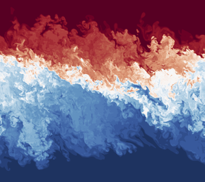
Figure 6 shows vertical slices of buoyancy (in figure 6a,d), the log of kinetic energy dissipation rate (in figure 6b,e) and the log of buoyancy variance dissipation rate (in figure 6c,f) at the spanwise centreline as in figure 4 but at two different times in simulation  $I$ (denoted by the vertical dashed and dotted lines in figure 5).

Figure 6. Vertical  $x$–
$x$– $z$ slices at $y=7.5$ of: (a,d) buoyancy $b$; (b,e) log of kinetic energy dissipation rate $\log _{10} ( \varepsilon )$; and (c,f) log of buoyancy variance dissipation rate $\log _{10} ( \chi )$ for simulation $I$ with ${Ri}_{0} = 0.1$ at two different times: data from a scouring event (a–c, marked with a dashed line in figure 5; data from an overturning event (d–f, marked with a dotted line in figure 5)).
Figure 6(d–f) shows slices taken at the time marked with a grey dotted line in figure 5, at (non-dimensional)  $t \approx 1000$ when the density interface is broadening. Coherent overturns of the density interface are visible and strong momentum dissipation is co-located with strong buoyancy gradients. This is qualitatively similar to figure 4(a–c) for simulation $B$. However, here the buoyancy interface, while broader than in the scouring-like state in figure 6(d–f), is still noticeably thinner than in simulation $B$. Figure 6(a–c) shows slices taken at the time marked with the grey dashed line in figure 5, at $t \approx 500$ when the density interface is thinning. Here, the buoyancy interface is thinner than in figure 6(d–f), and significant kinetic energy dissipation occurs on either side of the buoyancy interface, similar to figure 4(d–f) for simulation $T$ (although the interface is not quite as thin as in simulation $T$).
$T$).
Although this is an idealized system with  ${Pr} = 1$ and a relatively modest Reynolds number, it is interesting to note that the intense braid-like structures in the dissipation field of panel (e) strongly resemble the features in acoustic backscatter images of a salt-stratified estuarian outflow in figures 2 and 3 in Geyer et al. (Reference Geyer, Lavery, Scully and Trowbridge2010). Although they do not explicitly measure dissipation, they estimate kinetic energy dissipation from the vertical velocity variance measurements they make. In both Geyer et al. (Reference Geyer, Lavery, Scully and Trowbridge2010) and the overturning phase simulation $I$ here, the most intense dissipation values occur in regions of large buoyancy gradients. A similar co-location of intense kinetic energy and buoyancy variance dissipation can also be seen in the estuarian observations of Holleman, Geyer & Ralston (Reference Holleman, Geyer and Ralston2016), where again, they have not directly measured either dissipation, but rather estimated it from variance measurements.
3.3. Turbulent kinetic energy
Modifying the Osborn (Reference Osborn1980) assumption of stationarity in time and homogeneity in space to include forcing, the turbulent kinetic energy (TKE) equation reduces to a balance between four terms: shear production  $\mathcal {P}$, turbulent buoyancy flux $\mathcal {B}$, viscous dissipation $\mathcal {D}$ and forcing $\mathcal {F}$. These are defined as
 \begin{equation} \mathcal{P}(z) = - \left\langle \frac{\partial \langle u \rangle_{xy}}{\partial z} \langle u^{\prime} w^{\prime} \rangle_{xy} \right\rangle_t , \quad \mathcal{B}(z) = \langle b^{\prime} w^{\prime} \rangle_{xyt}, \end{equation}
 \begin{equation} \mathcal{D}(z) = \langle \varepsilon \rangle_{xyt}, \quad \mathcal{F}(z) = \langle u^{\prime 2} \rangle_{xyt} / \tau , \end{equation}
where  $u^{\prime }$, $w^{\prime }$ and $b^{\prime }$ are the fluctuations about $\langle u \rangle _{xy}$, $\langle w \rangle _{xy}$ and $\langle b \rangle _{xy}$, respectively. Figure 7 shows the horizontal and time averages of these four terms for the $B$ and $T$ cases. Case $I$ is not shown as stationarity is not achieved at any point in the simulation. Time averages are performed over the last 600 (non-dimensional) time units of the respective simulations. The average TKEs over this period for the $B$ and $T$ cases are $0.64 \pm 0.1$ and $0.015 \pm 0.0007$, respectively, and the average changes in TKE in time over this period are $0.0 \pm 0.004$ and $0.0 \pm 0.0003$, respectively, showing that a statistical steady state is maintained. Additionally, the magnitude of the forcing terms are less than half of the respective TKE production terms in each case.

Figure 7. Horizontal and time average of: shear production  $\mathcal {P}$; buoyancy flux $\mathcal {B}$; dissipation $\mathcal {D}$; and forcing $\mathcal {F}$; as a function of depth $z$ for (a) simulations $B$ with $Ri_{0} = 0.0125$ and (b) simulations $T$ with $Ri_{b,0} = 0.35$. The time average is performed over the last 600 (non-dimensional) time units of each respective simulation.
4. Linear stability analysis
In order to examine the initial and temporal evolution of the stability of each simulation, we have numerically calculated the linear stability of a viscous, diffusive, stratified shear flow system. We substitute the perturbation solutions
 \begin{equation} \boldsymbol{u} = U(z)\boldsymbol{i} + \epsilon \boldsymbol{u}^{\prime}(x,y,z,t), \quad b = B(z) + \epsilon b^{\prime}(x,y,z,t), \end{equation}
into (2.1)–(2.3) and linearize around the base states  $U$ and $B$. Considering normal modes of the form
 \begin{equation} \phi^{\prime}(x,y,z,t) = \hat{\phi}(z) \exp{\left[\sigma t + \textrm{i}kx\right]}, \end{equation}
where  $\phi ^{\prime }$ is the perturbation of any flow property, $\hat {\phi }(z)$ is the $z$-dependent eigenfunction, $\sigma$ is the growth rate and $k$ the streamwise wavenumber, we get the following system of forced, viscous Taylor–Goldstein equations
 \begin{equation} \sigma \left[\begin{array}{@{}cc@{}} \nabla^{2} & 0 \\ 0 & I \end{array} \right] \left[\begin{array}{@{}c@{}} \hat{w} \\ \hat{b} \end{array} \right] = \boldsymbol{A} \left[\begin{array}{@{}c@{}} \hat{w} \\ \hat{b}, \end{array} \right], \end{equation}
where
 \begin{equation} \left. \begin{gathered} A_{11} = -\textrm{i} k U \left({D}^{2} - k^{2} \right) + \textrm{i} k {D}^{2} U + \frac{1}{{Re}} \left({D}^{2} - k^{2} \right)^{2} + \frac{1}{\tau} {{D}}^{2},\\ A_{12} = -k^{2} {Ri}_0 ,\\ A_{21} = -\frac{\textrm{d} B}{\textrm{d} z} ,\\ A_{22} = -\textrm{i} k U + \frac{1}{{Re} {Pr}} \left({{D}}^{2} - k^{2} \right) + \frac{1}{\tau}, \end{gathered} \right\} \end{equation}
and  ${D}^{2} = \textrm {d}^{2}/\textrm {d}z^{2}$. The notable addition to this system of equations is the $\tau$ forcing terms. Boundary conditions at the top and bottom for $\hat {w}$ and $\hat {b}$ are free-slip and insulating, respectively. The base states $U$ and $B$ take the same form as the initial velocity and buoyancy profiles given in (2.6) and (2.7) covering a ${Ri}_0-R_0$ phase space through variation in the strength and depth of the buoyancy interface. We solve the system of equations using the procedure outlined in the appendix of Smyth, Moum & Nash (Reference Smyth, Moum and Nash2011). The most unstable mode is extracted for a range of $R_0$ and ${Ri}_0$ values. Figure 8 shows in colour the magnitude of the real part of the growth rate of the most unstable mode according to the linear stability analysis as a function of $R_0$ and $\log _{10} ( {Ri}_0 )$. Blue shading is used when the phase speed of the most unstable mode is zero (interpreted as being of KHI type) and the red shading is used when there is a complex conjugate pair with non-zero phase speeds of most unstable modes (interpreted as being of HWI type). Stable or neutral modes are coloured white. The initial condition $({Ri}_0,R_0)$ for simulation $B$ is marked with a triangle, for simulation $I$ is marked with a star, and simulation $T$ is marked with a square. The attached lines show the temporal evolution of each simulation in $Ri_b{-}R$ phase space. At each instant the updated values of $d$ and $\delta$, determined using (3.1) and (3.2), are used to determine the value of $R=d/\delta$ for the simulation, used as the $y$-coordinate on the figure. Analogously, we can also define a time-dependent value of the bulk Richardson number, taking into account the fact that the depth $d$ of the velocity interface in general increases (and so the intensity of the shear drops). We generalize the definition of the initial ${Ri}_0$ in (2.8a–d) as it has no time-dependent terms ( $d_0^{*}$ is defined as the initial velocity interface and so we distinguish it from the ${d}(t)$ used in (3.1)), so that
 \begin{equation} {Ri}_b(t)= \frac{{B}_0^{*} {d}_0^{*} \,{d}(t)}{({U}_0^{*})^{2}}= {Ri}_{0} \,{d}(t),\end{equation}
which we use to determine the  $x$-coordinate on the figure. Increases in $d>1$ lead inevitably to increases in ${Ri}_b$ from its initial value ${Ri}_0$. The grey lines denote the initial transitory, non-steady evolution of each simulation and the black lines show the steady or fully evolved state of each simulation. All three simulations exhibit an initial transient period that involves the broadening of the velocity interface. In simulation $B$, this broadening affects the velocity and buoyancy interfaces, so ${Ri}_b$ increases significantly (due to the increase in $d$) and the velocity and buoyancy interfaces becoming approximately equal in depth, and so $R \simeq 1$. In simulation $T$, while there is an initial broadening of both interfaces with $\delta$ increasing more than $d$,
$d$,  $R$ still remains substantially larger than in simulation $B$ (
$B$ ( $R \simeq 3.5$) once steady-state is achieved. Simulation $I$ resembles simulation $B$ in its low steady-state average $R$ value, however, unlike simulation $B$, simulation $I$ oscillates in phase space between two different states (examples of which can be seen in figure 6). Performing the same stability analysis as before, but using the instantaneous horizontally averaged velocity and buoyancy profiles at each time step output as the base state reveals that it is oscillating between a completely stable state and a state that is most unstable to a mode 2 KHI. However, caution should be taken in inferring the stability of the flow from these averaged profiles as the background state is continuously altered by the growing perturbations (Hogg & Ivey Reference Hogg and Ivey2003). Although ${Pr} = 1$ in these simulations, to leading order the forcing counteracts any broadening effects of the much slower molecular diffusion. Thus, turbulence is the primary mechanism for interface broadening and setting of the steady-state $R$ value here.

Figure 8. Growth rate  ${\rm Re}(\sigma )$ of the fastest growing mode from a linear stability analysis as a function of interface half-depth ratio $R_0=d_0/\delta _0$ and $\log _{10} ({Ri}_0)$. Regions plotted using the blue colour map correspond to fastest growing modes with zero phase speeds (i.e. unstable to KHI) and those using the red colour map correspond to fastest growing modes with non-zero phase speeds (i.e. unstable to HWI). The symbols ( $\text {triangle} = B$, $\text {star} = I$ and $\text {square} = S$) indicate the chosen parameters for the initial conditions of each of the simulations. The thick lines are the horizontally averaged trajectories for each simulation that the time-dependent parameters ${Ri}_b={Ri}_0 d$ and $R=d/\delta$ follow in time during the simulation using: grey lines trace the initial unsteady-state path; black lines trace the quasi-steady states (simulations $B$ and $T$) or spatio-temporally intermittent state (simulation $I$).
$I$).
5. Quantitative analysis
5.1. Mixing efficiency: physical coordinate space
Figure 9 shows as a function of time the horizontal averages of kinetic energy dissipation rate  $\langle \varepsilon \rangle _{xy}$, buoyancy variance dissipation rate $\langle \chi \rangle _{xy}$, and the associated mixing efficiency $\eta (z,t)$, defined as
 \begin{equation} \eta(z,t)\equiv \frac{\langle \chi \rangle_{xy}}{\langle \chi \rangle_{xy} + \langle \varepsilon \rangle_{xy}}, \end{equation}
for all three simulations. One advantage of this definition is that the mixing efficiency is a function of depth, unlike the mixing efficiency defined with the irreversible buoyancy flux as calculated from the available potential energy (APE) framework from Winters & D'Asaro (Reference Winters and D'Asaro1996) which yields a single volumetric mixing efficiency. For ease of comparison between different simulations,  $z$ has been normalized for each simulation by a time-averaged buoyancy interface half-depth $\langle \delta \rangle _{xyt}$ given by (3.2), where the time-averaged value is shown in each figure. For simulation $B$, we see that $\eta (z,t)$ is quite variable in space and time. Close to the midplane of the computational domain, $\eta (z,t)$ is relatively low, where overturning and turbulence is relatively active and thus $\langle \varepsilon \rangle _{xy}$ is large, but buoyancy is, relatively, more homogenized, so $\langle \chi \rangle _{xy}$ is somewhat suppressed. The mixing efficiency then increases to higher values toward the outer flanks of the turbulent region, where both $\langle \varepsilon \rangle _{xy}$ and $\langle \chi \rangle _{xy}$ become quite small. In contrast, simulation $T$ has a relatively constant mixing efficiency concentrated around the midplane of the computational domain, with peak values of the mixing efficiency and overall values of the kinetic energy dissipation and buoyancy variance dissipation much less than those in simulation $B$. However, a reduction or enhancement in mixing or mixing efficiency when comparing the two regimes, B and $T$, is not the only important point to be made here. As will be discussed in subsequent sections, how the mixing and mixing efficiencies vary with respect to the buoyancy interface in each regime is a key feature of that respective regime. Again, the high frequency oscillations seen in panels (c), (f) and (i) for simulation $T$ are a result of high frequency internal waves propagating along the density interface. These are effectively interfacial waves in the continuously stratified system and they can be seen more clearly in figure 4(d–f). Similarly to before, simulation $I$ appears to exhibit behaviour similar to aspects of both simulation $B$ and $T$, cycling between a state of high peak values towards the flanks and a state of lower, yet more uniform values that are localized around the midplane.

Figure 9. Horizontal averages of (a–c) kinetic energy dissipation rate [ $\log _{10}( \langle \varepsilon \rangle _{xy} )$]; (d–f) buoyancy variance dissipation rate [ $\log _{10}( \langle \chi \rangle _{xy} )$]; and (g–i) mixing efficiency [ $\eta = \langle \chi \rangle _{xy} / ( \langle \chi \rangle _{xy} + \langle \varepsilon \rangle _{xy} )$] as a function of time-averaged buoyancy-interface normalized depth $z/\langle \delta \rangle {xyt}$ and time $t$ for: simulation $B$ with $Ri_{0} = 0.0125$ (a,d,g); simulation $I$ with $Ri_{0} = 0.1$ (b,e,h); simulation $T$ with $Ri_{b,0} = 0.35$ (c,f,i). Horizontally and time-averaged buoyancy-interface half-depth $\langle \delta \rangle _{xyt}$ values used in normalizing $z$ for each simulation are averaged over the time window in each respective panel and are shown in white text at the tops of the panels in (b,e,h).
An important hypothesis of self-organization and the tendency for a system to be attracted towards critical  ${Ri}_g$ and $\eta$ values of 1/4 and 1/6 respectively at steady state is raised in Salehipour et al. (Reference Salehipour, Peltier and Caulfield2018) using data from unforced, initial-value simulations. To examine whether a forced system, such as the ones examined here, exhibits evidence of this behaviour we plot in figure 10 the probability density function (PDF) of the horizontally averaged gradient Richardson number and mixing efficiency as defined in (2.9) and (5.1), respectively. Data points included in the binning are from the interface region $-\langle \delta \rangle _{t}\leq z \leq \langle \delta \rangle _{t}$ and the last 600 (non-dimensional) time units of each simulation. As to be expected, simulation $B$ has relatively low gradient Richardson numbers and mixing efficiencies, simulation $T$ has relatively high gradient Richardson numbers and mixing efficiencies, and simulation $I$ is situated between the two. Although there is a peak at ${Ri}_g = 1/4$ in the steady state of simulation $T$, the mixing efficiencies are well above 1/6, and again, although there is a peak at $\eta = 1/6$ in the spatio-temporally intermittent simulation $I$, the gradient Richardson's number values are well below 1/4. Additionally, the majority of the steady-state values in simulation $B$ for both ${Ri}_g$ and $\eta$ are well below 1/4 and 1/6, respectively. We might not expect to find evidence of a self-organized basin of attraction here, as the forcing appears to act somewhat against these effects, not least due to being somewhat too strong for the underlying assumptions of the self-organized criticality paradigm.

Figure 10. Probability density function (PDF) of horizontally averaged (a) gradient Richardson number as defined in (2.9) and (b) mixing efficiency as defined in (5.1). Data plotted are from successive horizontal averages spaced 1 (non-dimensional) time unit apart across the respective time window shown in figure 9 within the region  $-\langle \delta \rangle _{t}\leq z \leq \langle \delta \rangle _{t}$. Red bars are from simulation $B$ with ${Ri}_{0} = 0.0125$; blue bars are from simulation $T$ with ${Ri}_{0} = 0.35$; green bars are from simulation $I$ with ${Ri}_{0} = 0.1$. Vertical dashed line in panel (a) marks ${Ri}_g = 1/4$ and in panel (b) $\eta = 1/6$.
5.2. Mixing efficiency: buoyancy coordinate space
The above view of the mixing efficiency, however, does not reveal the full picture. Horizontally averaging over the domain and thus the interfacial internal waves arising in both simulation  $T$ and $I$ produces a broad density interface when calculated in this fashion. In order to eliminate this misleading property, we now average the dissipation rate, buoyancy variance destruction rate, and mixing efficiency data based on the reference $z_*$ buoyancy coordinate space of Winters & D'Asaro (Reference Winters and D'Asaro1996) and Nakamura (Reference Nakamura1996). Specifically, the sorted buoyancy profile $b_*(z_*,t)$ is first calculated using the PDF method in Tseng & Ferziger (Reference Tseng and Ferziger2001). Then $\left \langle \epsilon \right \rangle _*$ and $\left \langle \chi \right \rangle _*$ are calculated by averaging the values of $\epsilon$ and $\chi$ that fall within a given $z_*$ bin.
For all three simulations, figure 11 plots (with thick lines) time and buoyancy coordinate-averaged kinetic energy dissipation rate  $\langle \varepsilon \rangle _{*t}$, buoyancy variance dissipation rate $\langle \chi \rangle _{*,t}$ and the associated time-averaged mixing efficiency $\langle \eta \rangle _{*,t}$, where $\eta _*$ is defined as
 \begin{equation} \eta_* \equiv \frac{\langle \chi \rangle_{*}}{\langle \chi \rangle_{*} + \langle \varepsilon \rangle_{*}}. \end{equation}
Time averages are performed using snapshots spaced 100 (non-dimensional) time units apart across the respective time windows shown in figure 9. Analogously to figure 9, for each simulation, the  $z_*$ coordinate is scaled with an appropriate measure of the depth of the buoyancy interface. Specifically, the time-dependent half-depth $\delta _*(t)$ of the buoyancy interface in buoyancy coordinate space is defined as
 \begin{equation} \delta_* (t) = \int_{-L_z/2}^{L_z/2} (1 - b_*^{2})\mathrm{d}z_* . \end{equation}
We then scale the vertical coordinate in the plots using the time average  $\langle \delta _*\rangle _t$, averaged over the same period as $\langle \varepsilon \rangle _*$, $\langle \chi \rangle _*$ and $\eta _*$, and the specific values of this quantity for each simulation are given on the figure. Furthermore, the data from simulation $I$ have been split to construct a time average, referred to as $I_B$, over all relatively thick interfaces, identified as interfaces for which $\delta _* > 2.4$ (the time-averaged values of $\delta _*$ for all of simulation $I$), and a time average, referred to as $I_T$, over all relatively thin interfaces, identified as interfaces for which $\delta _* < 2.4$. Finally, the shaded regions indicate $\pm 1$ standard deviation of the instantaneous data about the time average.

Figure 11. Average in time and sorted buoyancy coordinates  $z_*/\langle \delta \rangle _{*,t}$ of (a) kinetic energy dissipation rate $\log _{10}( \langle \varepsilon \rangle _{*,t} )$; (b) buoyancy variance destruction rate $\log _{10}( \langle \chi \rangle _{*,t} )$; and (c) mixing efficiency $\langle \eta \rangle _{*,t} = \langle \chi \rangle _{*,t} / ( \langle \chi \rangle _{*,t} + \langle \varepsilon \rangle _{*,t} )$ plotted with solid thick lines. Time averages are performed using data snapshots spaced 100 (non-dimensional) time units apart across the respective time window shown in figure 9. One standard deviation from this average is plotted with shaded regions and solid thin lines for: simulation $B$ with $Ri_{0} = 0.0125$ (red lines); simulation $I$ with $Ri_{0} = 0.1$ during the $I_T$ phase (grey lines) and $I_B$ phase (green lines); simulation $T$ with $Ri_{0} = 0.35$ (blue lines). The $I_T$ phase is defined by $\delta _* < 2.4$, while the $I_B$ phase is defined by $\delta _* > 2.4$. The time-averaged values of $\delta _*$ used are displayed in their respective colours.
Averaged in this way, it is now apparent that the dissipation in simulation  $T$ is localized on the edges of the buoyancy interface, exterior to the location of the strongest buoyancy gradient, the time average of which is maximum at the midpoint in $z_*$ coordinates. The kinetic energy dissipation rate is low in simulation $T$ in the region $-0.5\langle \delta _*\rangle _{t}\leq z_* \leq 0.5\langle \delta _*\rangle _{t}$ compared to the other simulations. The buoyancy variance destruction rate, $\langle \chi \rangle _*$, is also smaller near $z_*=0$ in simulation $T$, but the reduction compared to the other simulations is smaller and hence the mixing efficiency is relatively large in this region in simulation $T$. So while the midplane mixing efficiency is relatively large for simulation $T$, the flow at the midplane is quasi-laminar and mixing and $\langle \chi \rangle _*$ are at least an order of magnitude smaller than the other simulations at the midplane. However, when moving away from $z_*=0$ towards the flanks of the buoyancy interface, the flow becomes more turbulent. Both $\langle \varepsilon \rangle _*$ and $\langle \chi \rangle _*$ begin to increase for larger values of $z_*$ in simulation $T$, indicating more mixing is occurring, but do so in such a way that the mixing efficiency decreases. This difference between mixing at the midplane and flanks is precisely what contributes to the thinning of the interface in simulation $T$, as will be discussed further in § 5.3. Conversely, in simulation $B$, the maximum dissipation rate is co-located with the maximum buoyancy variance destruction. Additionally, both are spread across a much larger portion of the domain (of width $\langle \delta _* \rangle _t = 10.3$), leading a more broad and relatively moderate value of mixing efficiency. Subdividing simulation $I$ into $I_T$ and $I_B$ phases, it is apparent the associated mixing efficiencies are quite similar, exhibiting a combination of behaviours characteristic of both simulation $T$ and $B$. Specifically, dissipation is not peaked on the flanks of the buoyancy interface as in simulation $T$, but rather both dissipation and buoyancy variance destruction are peaked at the midpoint as in simulation $B$. On the other hand, the widths of these regions of enhanced dissipation and buoyancy variance dissipation (of width $\langle \delta _* \rangle _t = 2.0$ and $2.8$ respectively), are quite narrow, similarly to the observed behaviour in simulation $T$.
$T$.
A further depth-averaged mixing efficiency is calculated using an average across the buoyancy interface (i.e. for  $- \langle \delta _* \rangle _t < z_* < \langle \delta _* \rangle _t$), which we denote as $\overline {\eta _*}$. For simulations $B$ and $T$, the associated averaged values are $\overline {\eta _*}=0.11$ and $\overline {\eta _*}=0.43$ respectively, suggesting that, although it spans a much smaller vertical extent, simulation $T$ achieves a much higher interfacial-averaged mixing efficiency. However, a key point to keep in mind when considering the destruction or maintenance of sharp buoyancy interfaces, is not so much whether mixing and mixing efficiency are high or low overall when comparing simulation $B$ and $T$, but how mixing and mixing efficiency vary along the depth of the interface within each simulation (a point that is illustrated further in § 5.3). Evaluating mixing or mixing efficiency as a single depth-averaged value in simulations such as these can mask this important information. For simulation $I$, the value associated with the $I_T$ phase is $\overline {\eta _*}=0.23$ and the value associated with the $I_B$ phase is $\overline {\eta _*}=0.28$, falling between the values associated with the other two simulations.
5.3. Effective diffusivity
In examining the mechanisms behind the destruction or maintenance of buoyancy interfaces in layered stratified plane Couette flow simulations, Zhou et al. (Reference Zhou, Taylor, Caulfield and Linden2017b) derived an evolution equation for the buoyancy gradient in the same sorted buoyancy coordinate as discussed above. They found that the curvature of the effective diffusivity  $\kappa _e$, defined as
 \begin{equation} \frac{\partial^{2} \kappa_e}{\partial z_*^{2}} = \frac{\partial^{2}}{\partial z_*^{2}} \left[ \kappa^{*} \left( \frac{\partial z_*}{\partial b} \right)^{2} \langle \left| \boldsymbol{\nabla} b \right|^{2} \rangle_{z_*} \right] = \frac{\partial^{2}}{\partial z_*^{2}} \left[ \kappa^{*} \left( \frac{A_s}{A} \right)^{2} \right], \end{equation}
where  $A_s$ is the area of the isopycnal surface and $A$ is the area of the isopycnal surface projected onto a flat plane, served as a simple quantity to diagnose whether ‘scouring’ or ‘overturning’ processes took place at the interface. In this context, ‘scouring’ is characterized by positive curvature, while ‘overturning’ is characterized by negative curvature. The distinction can perhaps be best understood through consideration of isopycnal surfaces. Large overturning processes distort isopycnal surfaces near the midpoint, leading to a relatively large $A_s/A$ ratio and hence relatively large $\kappa _e$. This distortion then decreases away from the midpoint, creating negative curvature in $\kappa _e$. Conversely, during scouring processes, relatively large isopycnal distortion due to turbulence, and associated relatively large $A_s/A$, is displaced to either side of the interface, while at the midpoint (i.e. where $z_*=0$) the isopycnals are almost flat. This leads to a positive curvature in $\kappa _e$ and a mechanism by which diffusive spreading of the interface is counteracted. In addition to the curvature of $\kappa _e$, Prandtl number effects were also found to be important, as $\kappa _e$ is bounded below by the molecular value of $\kappa ^{*}$, which thus limits the development of positive curvature at finite Péclet numbers.
While the physical set-up of the Zhou et al. (Reference Zhou, Taylor, Caulfield and Linden2017b) simulations is quite different from that of this study, we can still employ this simple metric describing the curvature of  $\kappa _e$ to understand the mechanisms behind the interface broadening and thinning behaviour observed in simulations $B$,
$B$,  $T$ and $I$. In figure 12(c) we have plotted the time-averaged vertical profiles of $\kappa _e/\kappa ^{*}$ as a function of $z_*/\langle \delta _* \rangle _t$ for all three simulations. Time-averaging is the same as in figure 11. In simulation $B$,
$B$,  $\kappa _e$ is enhanced well above molecular diffusion across the entire depth of the domain with $\kappa _e$ exhibiting a negative curvature. Isopycnal distortion is greatest at the midpoint (i.e. at $z_*=0$) due to overturns, which naturally leads to interface broadening.

Figure 12. Variation with normalized buoyancy depth  $z_*/\langle \delta _* \rangle _t$ of the time-averaged (a) buoyancy Reynolds number $\langle {Re}_{b,*} \rangle _t$; (b) turbulent flux coefficient $\langle \varGamma _* \rangle _t$; and (c) normalized effective diffusivity $\kappa _e/\kappa ^{*}$ as defined in (5.5a–d) for simulation $B$ with ${Ri}_{0} = 0.0125$ (red lines); simulation $I$ with ${Ri}_{0} = 0.1$ during the $I_T$ phase (grey lines) and $I_B$ phase (green lines); simulation $T$ with ${Ri}_{0} = 0.35$ (blue lines). The $I_T$ phase is defined by $\delta _* < 2.4$, while the $I_B$ phase is defined by $\delta _* > 2.5$. Time averages are performed in the same manner as in figure 11 and respective time-averaged values of $\delta _*$ are the same as used in figure 11.
In simulation  $T$,
$T$,  $\kappa _e \simeq \kappa ^{*}$ for $|z_*|<\langle \delta _* \rangle _t$. Since $\kappa _e$ includes molecular diffusion, this indicates that there is very little enhancement in mixing by turbulence and the flow is quasi-laminar. For $|z_*|=\langle \delta _* \rangle _t$, $\kappa _e>2\kappa ^{*}$. Although this is smaller than in the other simulations, the enhancement of mixing by turbulence outside of the density interface is non-trivial. As a result of the enhanced mixing on the flanks of the density interface, the $\kappa _e(z_*)$ profile has positive curvature, and based on the analysis in Zhou et al. (Reference Zhou, Taylor, Caulfield and Linden2017b), this acts to thin the interface.
In Zhou et al. (Reference Zhou, Taylor, Caulfield and Linden2017b), similar thinning and broadening interfaces were seen. However, the interface thinning observed in that study required a relatively large Prandtl number ( $Pr=70$) to limit the diffusion of the interface. In the study described herein, the forcing plays a somewhat analogous role in limiting secular spreading of the interface. In all cases the velocity and buoyancy-interface depths are greater than their initial depths. The forcing term always works to counteract the effects of interface diffusion. In simulation $B$, this effect is swamped by the broadening effects of the overturns. On the other hand, in simulation $T$, the forcing helps the scouring eddies to maintain a thinner interface.
In order to understand what sets the magnitude of  $\kappa _e$, it is helpful to consider the following relation from Salehipour & Peltier (Reference Salehipour and Peltier2015) and Taylor & Zhou (Reference Taylor and Zhou2017) for $\kappa _e$, quantifying the effective diffusivity enhancement above the molecular $\kappa ^{*}$
 \begin{equation} \frac{\kappa_e}{\kappa^{*}} = {Pr} \varGamma_* {Re}_{b,*} + 1;\quad {Re}_{b,*} = \frac{\langle \varepsilon \rangle_*}{\nu^{*} N^{2}_*};\quad \varGamma_* = \frac{\eta_* }{\left( 1 - \eta_* \right)};\quad N^{2}_*=Ri_0\frac{\partial}{\partial z_*} b_* , \end{equation}
where  ${Re}_{b,*}$, $N^{2}_*$ and $\varGamma _*$ are a buoyancy Reynolds number, buoyancy frequency and turbulent flux coefficient constructed from the appropriately sorted buoyancy field $b_*(z_*,t)$, and generically functions of both $z_*$ and time.
Figure 12(a,b) shows time-averaged profiles of the buoyancy Reynolds number ( $\langle {Re}_{b,*} \rangle _t$) and flux coefficient ( $\langle \varGamma _* \rangle _t$) as a function of $z_*/\langle \delta _* \rangle _t$ for the three simulations. Again, time averaging is the same as in figure 11 and for $\kappa _e$ in panel (c). Comparing these profiles with their corresponding $\kappa _e$ profiles in panel (c), it is apparent that both $\langle {Re}_{b,*} \rangle _t$ and $\langle \varGamma _* \rangle _t$ contribute to the magnitude of $\kappa _e$. For simulation $B$,
$B$,  $\langle {Re}_{b,*} \rangle _t$ is relatively large over the entire depth of the domain, but $\langle \varGamma _* \rangle _t$ conversely is relatively small. The overturns are not particularly efficient at buoyancy variance destruction, at least partly because there is less buoyancy variance to destroy, but are nevertheless quite vigorous and thus lead to a relatively large value of $\kappa _e$. Conversely, in simulation $T$,
$T$,  $\langle {Re}_{b,*} \rangle _t$ is relatively small at the interface and increases away from it, while $\langle \varGamma _* \rangle _t$ is quite large at the interface and decreases away from it. Therefore, the scouring interface can be interpreted as being quite efficient at the destruction of buoyancy variance, but since overturns of the interface are suppressed, $\kappa _e$ falls to molecular $\kappa ^{*}$ values, and mixing at the interface is weak. Away from the interface, there is less buoyancy variance to destroy, but turbulence conversely become more vigorous and $\kappa _e$ is larger than at the interface. Again, the $I_T$ and $I_B$ phases of simulation $I$ lie somewhere in between simulations $B$ and $T$ at intermediate values and exhibit a mix of characteristics of the dynamics of the other two simulations.
Crucially, as is immediately apparent from panel (c), forced flows exhibiting overturning, broadening behaviour lead to much more diapycnal transport than flows exhibiting scouring, thinning behaviour. Although the mixing in simulation  $B$ may be thought of as being less efficient than in simulation $T$, since typical values of the flux coefficient $\varGamma _*$ are significantly smaller for simulation $B$ than for simulation $T$, this effect is completely swamped by the substantially higher average value of the buoyancy Reynolds number, as shown in panel (a) (and thus perhaps warrants a comparison to be made between scouring and overturning mechanisms at the same buoyancy Reynolds number). Therefore, from (5.5a–d), the overturning-dominated mixing in simulation $B$ has a much larger typical value of effective diffusivity than the scouring-dominated mixing in simulation $T$, remembering that the horizontal axes in the figure are logarithmic. It is also apparent that the intermediate simulation $I$ has properties which lie between the two other simulations, with significantly larger effective diffusivity when the flow is in the $I_B$ phase.
5.4. Scaling of mixing efficiency
There is mounting evidence that mixing associated with stratified turbulence is a function of one or more non-dimensional numbers (see e.g. Linden Reference Linden1979; Shih et al. Reference Shih, Koseff, Ivey and Ferziger2005; Brucker & Sarkar Reference Brucker and Sarkar2007; Karimpour & Venayagamoorthy Reference Karimpour and Venayagamoorthy2014; Holleman et al. Reference Holleman, Geyer and Ralston2016; Maffioli, Brethouwer & Lindborg Reference Maffioli, Brethouwer and Lindborg2016; Salehipour et al. Reference Salehipour, Peltier, Whalen and MacKinnon2016b; Venayagamoorthy & Koseff Reference Venayagamoorthy and Koseff2016; Zhou et al. Reference Zhou, Taylor, Caulfield and Linden2017b; Garanaik & Venayagamoorthy Reference Garanaik and Venayagamoorthy2019). Here, we diagnose the dependence of the time-dependent mixing efficiency  $\eta _*(z_*, t)$ in reference buoyancy coordinates (as defined in (5.2)) on several (also time-dependent) non-dimensional numbers to understand these relationships in a continuously forced system. As noted above, the actual (effective) diffusivity is proportional to the product of the turbulent flux coefficient $\varGamma _*=\eta _*/(1+\eta _*)$ and the buoyancy Reynolds number ${Re}_{b,*}$, and so any dependence of $\eta _*$ on ${Re}_{b,*}$ is naturally of interest to explain (and parameterize) the eventual effective diffusivity.
We use the results of our simulations to determine the values of various key quantities as functions of time and the reference buoyancy coordinate  $z_*$, and then construct various non-dimensional parameters on which (an appropriately defined) mixing efficiency has been hypothesized to depend. In particular, figures 13 and 14 show time-dependent mixing efficiency and flux coefficient with respect to several commonly considered non-dimensional numbers. Specifically, we are interested in the dependence on the buoyancy Reynolds number ${Re}_{b,*}$ as defined in (5.5a–d), gradient Richardson number and horizontal Froude number in the reference $z_*$ buoyancy space coordinate, defined as
 \begin{equation} {Ri}_{g,*} = \frac{N^{2}_*}{S^{2}_*}, \quad {Fr}_{h,*} = \frac{\varepsilon_*}{N_* {U}_{h,*}^{2}}, \end{equation}
where  $S^{2}_* = ( \langle {\partial u}/{\partial z} \rangle _* )^{2}$ and ${U}_{h,*} = \sqrt {\langle u^{\prime 2} + v^{\prime 2} \rangle _*}$. Here, the gradient for the shear is with respect to the physical space vertical coordinate and $u^{\prime }$ and $v^{\prime }$ are the fluctuating horizontal velocities calculated as departures from the horizontal means $\langle u \rangle _{xy}$ and $\langle v \rangle _{xy}$ in physical space.

Figure 13. Variation of mixing efficiency,  $\eta _*$ (as defined in (5.2)), with (a) buoyancy Reynolds number, $\log _{10}( {Re}_{b,*} )$; (b) gradient Richardson number, $Ri_{g,*}$; and (c) variation of the flux coefficient, $\varGamma _*$, with horizontal Froude number, $Fr_{h,*}$. Only points within the region $-\delta _* \leq z_* \leq \delta _*$ are shown. Red points are from simulation $B$ with ${Ri}_{0} = 0.0125$; blue points are from simulation $T$ with ${Ri}_{0} = 0.35$. Black and green points are from simulation $I$ with $Ri_{b,0} = 0.1$ during the $I_T$ phase and $I_B$ phase respectively. No time-averaging is performed. Instead, all data points are plotted from successive snapshots spaced 100 (non-dimensional) time units apart within the respective time window shown in figure 9. Shading indicates distance from $z_* = 0$, or neutral buoyancy, where light is close to $z_* = 0$ and dark is close to $z_* = \pm \delta _*$. In panel (a) the dashed line indicates $\eta _* \propto {Re}_{b,*}^{-{1}/{2}}$ scaling. In panel (b) the dashed line indicates $\eta _* \propto Ri_{g,*}$ scaling and the dotted line is $\eta _* = 0.25 [1- \exp (-7 Ri_{g,*}) ]$ scaling. In panel (c) the dashed line indicates $\varGamma _*\propto Fr_{h,*}^{-2}$ and the dotted line indicates $\varGamma _*\propto Fr_{h,*}^{-1}$. The vertical solid grey line in panel (c) marks the regime transition between the $\varGamma _* \propto Fr_{h,*}^{-2}$ scaling and constant $\varGamma _*$ found by Maffioli et al. (Reference Maffioli, Brethouwer and Lindborg2016).

Figure 14. Comparison of mixing efficiency,  $\eta _*$ (as defined in (5.2) and shown as symbol shading), as a function of buoyancy Reynolds number, $\log _{10}({Re}_{b,*} )$ and gradient Richardson number, $Ri_{g,*}$ within the region $-\delta _* \leq z_* \leq \delta _*$. As in figure 13, all data points are plotted from successive snapshots spaced 100 (non-dimensional) time units apart within the respective time window shown in figure 9 with no time averaging performed. Data from simulation $B$ with ${Ri}_{0} = 0.0125$ are plotted with triangles; simulation $T$ with ${Ri}_{0} = 0.35$ are plotted with squares; and from simulation $I$ with ${Ri}_{0} = 0.1$ are plotted with diamonds and circles for the $I_T$ phases and $I_B$ phases respectively. Note that the colour bar has been saturated at a value of 0.4 and for some value less than $\log _{10}({Re}_{b,*} )=1$ the mixing efficiency $\eta _*$ is always greater than 0.4. The dashed line plots a $Ri_{g,*} \propto 1/{Re}_{b,*}$ scaling.
In each case, all values of  $\eta _*$ over the range $-\delta _* \leq z_* \leq \delta _*$ are plotted against the relevant parameter and no time averaging is performed. Points outside of this $z_*$ range are not considered in this analysis because stratification in this region is very weak and our focus is on the properties of turbulence and mixing within a stratified shear layer. By restricting our analysis to the stratified interface, we are able to compare the three simulations more directly since the stratified interface occupies a much smaller fraction of the computational domain in simulations $T$ and $I$ than in simulation $B$. Data points are plotted from successive snapshots spaced 100 (non-dimensional) time units apart within the respective time window shown in figure 9. The colouring of circles indicates distance from $z_* = 0$, where light is close to $z_* = 0$ and dark is close to $z_* = \pm \delta _*$. A series of scaling lines are provided for reference on each of the panels. In figure 13(a), the dashed lines show the scaling $\eta _* \propto {Re}^{-1/2}_{b,*}$ identified in the DNS simulations of Shih et al. (Reference Shih, Koseff, Ivey and Ferziger2005) and field measurements of Davis & Monismith (Reference Davis and Monismith2011) and Walter et al. (Reference Walter, Squibb, Brock Woodson, Koseff and Monismith2014). The data appear to be consistent with a $\eta _* \propto {Re}^{-1/2}_{b,*}$ scaling for simulation $B$, which it must be remembered is relatively weakly stratified. We do not see evidence for an asymptote to a constant mixing efficiency for small ${Re}_{b,*}$ as suggested in Shih et al. (Reference Shih, Koseff, Ivey and Ferziger2005). However, the Reynolds number and resolution of the simulations in this study are not similar to those in Shih et al. (Reference Shih, Koseff, Ivey and Ferziger2005).
Shih et al. (Reference Shih, Koseff, Ivey and Ferziger2005) proposed that the mixing efficiency transitions from a constant value to  $\eta \propto {Re}_b^{-1/2}$ at ${Re}_b\simeq 100$. However, several recent studies have found that the value of ${Re}_b$ that marks the start of the $\eta \propto {Re}^{-1/2}_{b}$ scaling is Reynolds number dependent (Lozovatsky & Fernando Reference Lozovatsky and Fernando2013; Maffioli et al. Reference Maffioli, Brethouwer and Lindborg2016; Taylor et al. Reference Taylor, de Bruyn Kops, Caulfield and Linden2019). Extrapolating the ${Re}_{b,*}^{-1/2}$ scaling line in figure 13(a) suggests that the start of the ${Re}_{b,*}^{-1/2}$ scaling occurs for ${Re}_{b,*}>100$ in our simulations, although the gap between cases $B$ and $I_B$ make it difficult to be precise about this transition point. Additionally, the mixing efficiency does not appear to decay to zero at small values of ${Re}_{b,*}$, as was seen in the analysis of Salehipour & Peltier (Reference Salehipour and Peltier2015) which only included the post roll-up mixing events, but rather varies non-monotonically as ${Re}_{b,*}$ decreases. Specifically, $\eta _*$ decreases in the $I_T$ phase after an initial peak during the $I_B$ phase for simulation $I$, but it is observed to increase again in simulation $T$. Figure 2 in Mashayek, Caulfield & Peltier (Reference Mashayek, Caulfield and Peltier2017) shows that with the addition of the roll-up, denoted as ‘DNS: young’, a similar second peak in mixing efficiency at low ${Re}_{b,*}$ occurs.
The dependence of the mixing efficiency on the gradient Richardson number,  $Ri_{g,*}$ is shown in figure 13(b). For comparison, the dashed line shows the scaling $\eta _* \propto Ri_{g,*}$. As proposed by Salehipour & Peltier (Reference Salehipour and Peltier2015), this scaling arises from the assumption that an appropriate (irreversible) definition of the turbulent Prandtl number is unity, implying that the turbulent diffusivities of momentum and (irreversible) buoyancy variations are equal. As discussed in Salehipour & Peltier (Reference Salehipour and Peltier2015), this scaling follows by noting that the turbulent Prandtl number $Pr_{T,*}$ can be written as
 \begin{equation} Pr_{T,*}\equiv \frac{\nu_T(z_*,t)}{\kappa_T(z_*,t)}=\frac{-{\mathcal{P}}_*/S_*^{2}}{-{\mathcal{B}}_*/N^{2}_*}=\frac{{\mathcal{P}}_*}{{\mathcal{B}}_*} {Ri}_{g,*} \equiv \frac{{Ri}_{g,*}}{R_{f,*}}, \end{equation}
where  $R_{f,*}=R_{f,*}(z_*,t)$ is a ‘flux Richardson number’, and $\nu _T$ and $\kappa _T$ are the turbulent viscosity and diffusivity, respectively. They are defined as the ratio of the turbulent momentum (buoyancy) flux to the momentum (buoyancy) gradient. $\kappa _T$ here differs from the $\kappa _e$ used above as $\kappa _T$ vanishes in the limit of a laminar flow, while $\kappa _e$ remains non-zero due to molecular diffusion. For a quasi-steady state with negligible turbulent transport (see for example Mashayek, Caulfield & Peltier Reference Mashayek, Caulfield and Peltier2013; Salehipour & Peltier Reference Salehipour and Peltier2015 for further discussion) it is commonplace to assume that, particularly when only irreversible processes are considered, $R_{f,*}\simeq \eta _{*}$ or equivalently $R_{f,*}\simeq \varGamma _{*}/(1+\varGamma _{*})$. Therefore the assumption that both momentum and buoyancy are ‘mixed’ largely equivalently by turbulent motions and $Pr_{T,*}\simeq 1$, implies that $\eta _* \propto Ri_{g,*}$. There is increasing evidence for this scaling, particularly when a flow may be characterized as being relatively weakly stratified (see for example Zhou, Taylor & Caulfield Reference Zhou, Taylor and Caulfield2017a; Portwood, de Bruyn Kops & Caulfield Reference Portwood, de Bruyn Kops and Caulfield2019). On the other hand, the dotted line in figure 13 shows the essentially empirical scaling
 \begin{equation} \eta_* = 0.25 \left[1- \exp \left(-7 Ri_{g,*}\right) \right], \end{equation}
proposed by Karimpour & Venayagamoorthy (Reference Karimpour and Venayagamoorthy2014) and Venayagamoorthy & Koseff (Reference Venayagamoorthy and Koseff2016).
Simulations  $B$ and $I$ appear to exhibit at least approximate agreement with the unity turbulent Prandtl number scaling. Around $Ri_{g,*} \sim 0.2\text {--}0.25$ the data (largely the interface preserving data from simulation $T$) begins to deviate from this scaling. From here it is unclear as to whether $\eta _*$ asymptotes to a constant value, similar to the empirical scaling relation in (5.8), or if it decreases again in some fashion, as is predicted by the right flank of the flux-gradient curve within the paradigm presented by (Phillips Reference Phillips1972) for the development (and maintenance) of interfaces, and is observed in the experimental data presented by Linden (Reference Linden1979).
Although the flows considered here are forced specifically by a vertical shear, it is also of interest to compare the mixing efficiency with scalings proposed in terms of the horizontal Froude number,  $Fr_{h,*}$, which naturally is expressed in terms of properties of the turbulence and background stratification alone. Maffioli et al. (Reference Maffioli, Brethouwer and Lindborg2016) proposed that for sufficiently high Reynolds number, ${Re}$, the flux coefficient, $\varGamma$, is a function of the Froude number alone. Specifically, Maffioli et al. (Reference Maffioli, Brethouwer and Lindborg2016) proposed that
 \begin{equation} \varGamma_* \propto Fr^{-2}_{h,*},\quad \textrm{for}\ Fr_{h,*}>0.3, \end{equation}
and Garanaik & Venayagamoorthy (Reference Garanaik and Venayagamoorthy2019) proposed an additional intermediate scaling  $\varGamma _*\propto Fr_{h,*}^{-1}$ for $Fr_{h,*}=O(1)$, where in both cases we have written the scaling in terms of variables calculated in sorted buoyancy coordinates. Since the Reynolds number, buoyancy Reynolds number and Froude number are related through ${Re}_{b,*}={Re}Fr_{h,*}^{2}$ by definition (e.g. Ivey, Winters & Koseff Reference Ivey, Winters and Koseff2008), for fixed ${Re}$, the scaling $\varGamma _* \propto Fr_{h,*}^{-1}$ is equivalent to $\varGamma _* \propto Re_{b,*}^{-1/2}$.
Figure 13(c) shows the flux coefficient,  $\varGamma _*$, as a function of the horizontal Froude number, $Fr_{h,*}$, along with lines indicating $\varGamma _*\propto Fr_{h,*}^{-1}$ (dotted) and $\varGamma _*\propto Fr_{h,*}^{-2}$ (dashed). The solid grey line shows the regime transition from the scaling given in (5.9) for $Fr_{h,*} > 0.3$ to an $\eta \sim 0.23$ scaling for $Fr_{h,*} < 0.3$ seen by Maffioli et al. (Reference Maffioli, Brethouwer and Lindborg2016) in their steady-state forced shear-free DNS simulations. Simulation $B$ is consistent with a $Fr_{h,*}^{-1}$ scaling, while the scatter in the data points makes it difficult to determine whether the results follow a $Fr_{h,*}^{-2}$ scaling, although the data is not inconsistent with this scaling for $Fr_{h,*}>0.3$ as proposed by Maffioli et al. (Reference Maffioli, Brethouwer and Lindborg2016).
There is no significant evidence of an asymptote to a constant as proposed by Maffioli et al. (Reference Maffioli, Brethouwer and Lindborg2016) and Garanaik & Venayagamoorthy (Reference Garanaik and Venayagamoorthy2019) for small Froude numbers. However, our simulations differ from those reported in Maffioli et al. (Reference Maffioli, Brethouwer and Lindborg2016) in several important ways and are perhaps not expected to be directly comparable. First, the flows here are never ‘strongly’ stratified at all depths. Second, they are specifically designed to inject energy through shear instabilities, while those in Maffioli et al. (Reference Maffioli, Brethouwer and Lindborg2016) are isotropically forced. Third, the vertical Froude number here is somewhat constrained by the initial and forcing value of  $Ri_0$ and may not reach unity as it has in Maffioli et al. (Reference Maffioli, Brethouwer and Lindborg2016), where it no longer influences the dynamics. However, we argue that, in the flows considered here, the vertical momentum length scale (used in the calculation of the vertical Froude number) is not the only important length scale. Here, the width of the momentum and buoyancy interfaces, and in particular their ratio, $R$, is an important parameter, as demonstrated in figure 8.
In figure 13 the spatial variability within the buoyancy interface in the  $B$ and $I$ cases are quite small, meaning they are more robust to the different definitions of vertical averaging one might choose in order to arrive at an average measure of the mixing efficiency. In contrast, the $T$ case has a very strong dependence on depth within the buoyancy interface and thus would be quite sensitive to the specific choice in definition of vertical averaging. It should be noted for all of these scalings that the method used for averaging and the definition of each non-dimensional number could be different between the current study and those that are cited and thus could explain some of the differences.
Figure 14 shows the specific value of the mixing efficiency (shown as symbol shading), as defined in (5.2), as a function of  ${Re}_{b,*}$ and $Ri_{g,*}$. Data from simulation $B$ are plotted as triangles, from simulation $T$ are plotted as squares, while phase $I_B$ and phase $I_T$ from simulation $I$ are plotted with circles and diamonds respectively. Here again, no time or vertical averaging is performed. All data points are plotted from within the region $-\delta _* \leq z_* \leq \delta _*$ and from successive snapshots spaced 100 (non-dimensional) time units apart within the respective time window shown in figure 9. From this plot, it is clear that for all the simulations ${Re}_{b,*}$ and $Ri_{g,*}$ are correlated, and overall, a decrease in gradient Richardson number corresponds to an increase in the buoyancy Reynolds number, although there is some suggestion of an increase in $Ri_{g,*}$ with intermediate values of ${Re}_{b,*}$. An additional dashed line plots a $Ri_{g,*} \propto 1/{Re}_{b,*}$ scaling, which naturally emerges from their respective dependence on $N_*^{2}$. Such a scaling implies that turbulence is shear generated. Its properties are determined by the large scale shear and not strongly affected by the stratification. Thus in turn, the stratification is also not strongly affected by the turbulence. Both the $B$ and $T$ cases fall on this line because in their steady states, where turbulence is strong (everywhere for the $B$ case and on either side of the interface for the $T$ case), it is shear generated and stratification is relatively weak. In contrast, the $I$ case does not fall on the line because it is never in a steady state, instead the shear and stratification compete with each other. Thus turbulence is not solely shear generated and the stratification is not unaffected.
Non-monotonic variation of  $\eta _*$ with ${Re}_{b,*}$ is once again apparent, with peak values of $\eta _*$ shown for both simulation $T$ and the $I_B$ phase of simulation $I$. Also, the relatively high values of $\eta _*$ at very low ${Re}_{b,*}$ and high $Ri_{g,*}$ suggest that, even though entrainment of fluid due to large overturning processes may strongly decrease in a weakly turbulent flow with a robust interface, the flux of buoyancy, and associated irreversible mixing across the interface, is not fully suppressed. However, it is important to appreciate that such high efficiency does not imply large (total) transport, due to the associated small value of ${Re}_{b,*}$, thus implying from (5.5a–d) relatively little enhancement in (irreversible) effective diffusivity.
6. Conclusions
We have demonstrated the existence of three distinct types of behaviour in an idealized continuously forced, stratified shear flow: (i) a weakly stratified, broad density interface in simulation  $B$; (ii) a thin, strongly stratified density interface in simulation $T$; and (iii) spatio-temporal intermittency with certain characteristics of each of the other two behaviours, shown in simulation $I$. Each simulation had the same ${Re}=4000$, ${Pr}=1$ and initial $R_0=7$, the ratio between the initial velocity and buoyancy-interface half-depths, but different initial bulk Richardson numbers ${Ri}_0$.
Simulation  $B$ is characterized by turbulent eddies and overturns being largely co-located with strong buoyancy gradients. This flow structure leads to a relatively rapid break up and broadening of the buoyancy interface so that the ratio of the velocity and buoyancy-interface half-depths $R\approx 1$ throughout the quasi-steady-state flow evolution. In contrast, simulation $T$ is characterized by turbulent eddies being shifted slightly above and below the (robust) buoyancy interface. This produces a scouring effect, ensuring that the buoyancy interface remains relatively thin compared to the velocity interface, and so $R>1$ throughout the quasi-steady-state evolution of this simulation.
We have found that there is a useful classification in terms of a parameter space based on the specific properties of the initial and forced background velocity and buoyancy profiles, in particular the values of  ${Ri}_b$ and $R=d/\delta$, as defined in (4.5), (3.1) and (3.2). Certain regions of this parameter space can be associated with these two dynamically different behaviours, which may be characterized as ‘overturning’ and ‘scouring’ dynamics. Loosely, overturning dynamical behaviour is associated with relatively small values of ${Ri}_b$ and $R$, while scouring dynamical behaviour is associated with larger values of ${Ri}_b$ and $R$.
$R$.
However, we have also found that there is not a sharp transition between these two behaviours. For certain choices of initial parameters, as demonstrated by simulation  $I$, intermediate dynamical behaviour occurs, characterized by spatio-temporal intermittency and alternating overturning and scouring behaviour with points of at least qualitative similarity to simulations $B$ and $T$. As shown in figure 8, simulations $B$ and $T$ evolved to quasi-steady states, with characteristic values of associated bulk Richardson number ${Ri}_b$ and interfacial depth ratio $R$. Interestingly, linear stability analysis of the notional horizontally averaged background profiles of velocity and buoyancy reveals that the quasi-steady state of simulation $B$ is most unstable to Kelvin–Helmholtz-type instabilities, while the quasi-steady state of simulation $T$ is most unstable to Holmboe wave instabilities. These observations suggest that linear stability could be useful to determine if a quasi-steady forced turbulent system is in either an overturning or scouring state.
Comparison of the three forced simulations considered here to previously reported unforced (and hence inherently transient) simulations is instructive. For example, in the unforced KHI and HWI simulations of Salehipour et al. (Reference Salehipour, Caulfield and Peltier2016a) and Salehipour et al. (Reference Salehipour, Peltier and Caulfield2018), qualitatively similar overturning behaviour at low  $R$ values and scouring behaviour at higher $R$ values is observed, consistent with previous simulations at substantially smaller Reynolds numbers considered by Carpenter et al. (Reference Carpenter, Smyth and Lawrence2006). Indeed, all such simulations are consistent with the theoretical predictions of Smyth & Peltier (Reference Smyth and Peltier1991) and Hogg & Ivey (Reference Hogg and Ivey2003).
Furthermore, the HWI simulations of Salehipour et al. (Reference Salehipour, Caulfield and Peltier2016a) clearly exhibited both a scouring-like behaviour and a ‘long-lived twin-lobed’ structure in the diapycnal diffusivity. Recalling the simple metric of Zhou et al. (Reference Zhou, Taylor, Caulfield and Linden2017b) utilized here, the positive curvature of the diffusivity profile reported in Salehipour et al. (Reference Salehipour, Caulfield and Peltier2016a) suggests strong points of commonality between these (transient) simulations and the continually forced simulation  $T$ described here. This is perhaps unsurprising, since as discussed in Salehipour et al. (Reference Salehipour, Peltier and Caulfield2018), transient flows prone to HWI apparently approach for an extended period a quasi-equilibrium state. Perhaps more interestingly, in the inherently transient simulations prone to primary KHI, Salehipour et al. (Reference Salehipour, Caulfield and Peltier2016a) observed an analogously negative curvature in diapycnal diffusivity to simulation $B$ reported here. This point of similarity suggests that such a property may well be generic for flows prone to relatively large-scale overturning mixing.
As discussed in Salehipour et al. (Reference Salehipour, Caulfield and Peltier2016a), the efficiency of mixing by a KHI-dominated flow can reach substantially larger values compared to the mixing associated with a HWI-dominated flow with the same (initial) bulk Richardson number  ${Ri}_0=0.16$, and yet different initial interface ratio $R_0$, ( $R_0=1$ for the KHI simulation and $R_0=\sqrt {8}$ for the HWI simulation) principally due to the ‘flare’ associated with the large primary KHI billow overturning. They also found that ${Re}_{b,*}$ reached significantly larger values in the KHI-dominated flow, thus leading transiently to larger effective diffusivity $\kappa _e$ (see their figure 11). This behaviour is superficially not consistent with our forced results here, where the time-averaged mixing efficiency was much lower in the overturning simulation $B$ than in the scouring simulation $T$. However, it is important to remember that the initial bulk Richardson number is much smaller for simulation $B$ than for simulation $T$ (0.0125 as opposed to 0.35), and also that their simulations were at higher ${Pr}=8$. Furthermore, in our analysis here, we only consider the steady-state behaviour of the system, and in particular we ignore the collapse of the first overturning event in simulation $B$. Also, as is shown in figure 12, the effective diffusivity of simulation $B$ is still markedly larger than for simulation $T$, principally due to ${Re}_{b,*}$ being substantially larger in the broadening simulation, which does have points of consistency with the KHI-dominated simulation reported in Salehipour et al. (Reference Salehipour, Caulfield and Peltier2016a).
Additionally, we see higher mixing efficiency values at very low buoyancy Reynolds number here in comparison to the strongly stratified HW simulations of Salehipour et al. (Reference Salehipour, Caulfield and Peltier2016a), suggesting that the re-supply of stratification through the forcing helps to sustain a larger mixing efficiency. While this may be less relevant in the open ocean, it could be an important factor in natural exchange flows where there is an external source of buoyancy, although it is worth noting that if  ${Re}_{b,*}$ is small, the enhancement in diffusivity might not be significant.
Our demonstration of the scouring dynamics at relatively high Richardson numbers suggests that this behaviour could be a mechanism for interface formation and preservation in places where there are large buoyancy contrasts, such as the sharp thermoclines of estuaries. Additionally, the maintenance of a sharp interface at a relatively low Prandtl number in this study suggests that in regions of high levels of turbulence, such as those associated with many exchange flows, a high Prandtl number may not be necessary for either interface formation or maintenance if there is some form of external forcing and a re-supply of buoyancy. Indeed, a fluid with a larger Prandtl number should result in more of the  $Ri_b-R$ phase space being favourable for interface formation and maintenance.
Acknowledgements
This work was supported by funding from the Engineering and Physical Sciences Research Council (EPSRC) under the Programme Grant EP/K034529/1 ‘Mathematical Underpinnings of Stratified Turbulence’ (MUST) and the European Research Council (ERC) under the European Union's Horizon 2020 research and innovation Grant No 742480 ‘Stratified Turbulence And Mixing Processes’ (STAMP). The authors gratefully acknowledge many helpful discussions and suggestions from the MUST project team.
Declaration of interests
The authors report no conflict of interest.
Appendix. Dependence on $\tau$

In order to show the dependence of the results shown here on the chosen value of  $\tau$, additional simulations were run for $\tau = 50, 100$ and 200 for each of the three $Ri_0$ values. These simulations used a lower resolution than the simulations in the text and should be classified as under-resolved DNS. However, comparing the fully resolved and under-resolved simulations with $\tau =100$ shows that the qualitative behaviour is similar. Note that all results shown here for $\tau = 100$ are from the under-resolved simulations in order to make a fair comparison between the different $\tau$ value results. Specifically, the same physical dimensions, boundary conditions, and form of forcing were used, but the resolution was reduced to $256 \times 256 \times 128$ grid points and the value of $\tau$ was set to 50, 100 or 200.
Figure 15 shows the trajectories of the simulations in  $R$,
$R$,  $Ri_b$ phase space as in figure 8 in the main text, but now for $\tau = 50$, 100 and 200, differentiated by dashed, solid or dotted lines, respectively. Trajectories are calculated in the same way using (3.1) and (3.2) to construct a time-dependent $R$ and bulk Richardson number and the initial conditions are marked with a triangle for $Ri_0 = 0.0125$, a star for $Ri_0 = 0.1$ and a square for $Ri_0 = 0.35$. Linear stability analysis was performed for the three different values of $\tau$. While the magnitude of the growth rates of the fastest growing modes do vary with $\tau$, we found that the boundaries between the KHI, HWI and stable regions to be only very weakly dependent on $\tau$ within this range. Thus for simplicity and clarity, we choose to plot only the boundaries between the primary instability regimes for $\tau = 100$ here (which correspond closely to the boundaries for $\tau = 50$ and 200). The blue contour line denotes the boundary of the region where the most unstable mode is a KHI, the red contour line denotes the boundary of the region where the most unstable mode is a HWI, and all regions outside of both the red and blue contour lines are stable.

Figure 15. Boundaries of the positive growth rate  ${\rm Re}(\sigma )$ regions for the fastest growing mode from the $\tau = 100$ linear stability analysis (same as in figure 8) as a function of interface half-depth ratio $R_0=d_0/\delta _0$ and $\log _{10} ({Ri}_0)$. Regions to the left of the blue contour line correspond to where the fastest growing modes have zero phase speeds (i.e. unstable to KHI) and regions enclosed by the red contour line correspond to where the fastest growing modes have non-zero phase speeds (i.e. unstable to HWI). Regions outside of the blue and red contour lines correspond to where all modes are decaying (i.e. stable). Like figure 8, the symbols ( $\text {triangle} = B$, $\text {star} = I$ and $\text {square} = T$) indicate the chosen parameters for the initial conditions of each of the simulations. The thick black lines are the horizontally averaged trajectories for each under-resolved simulation that the time-dependent parameters ${Ri}_b={Ri}_0 d$ and $R=d/\delta$ follow in time during the simulation, with dashed lines corresponding to $\tau = 50$, solid lines to $\tau = 100$ and dotted lines to $\tau = 200$.
In general, we found that the simulations do not strongly depend on the value of  $\tau$ unless the flow changes regimes (e.g. from broadening to thinning). For $Ri_0 = 0.0125$, all of the results are largely insensitive to the range of $\tau$ values tested and behave largely the same. Similarly, for $Ri_0 = 0.35$, reducing the forcing time scale to 50 results in very similar behaviour to the $\tau = 100$ simulations. However, an increase in the forcing time scale to 200 causes a regime change, from one of interface thinning to one of interface broadening. For the $Ri_0 = 0.1$, a regime change does not occur, but the period and amplitude of the spatio-temporally intermittent pulsations was affected by changes in $\tau$. There appears to be a roughly linear relationship between the $\tau$ and the period of the pulsations, though this conclusion should be taken with caution as it is made with only three data points. Concerning differences in the transient behaviour dependence on $\tau$, we found that for all three values of $Ri_0$ the transient period was roughly the same for the different values of $\tau$ so long as a regime change was not triggered (as it was with $Ri_0 = 0.35$, $\tau = 200$).
In order to examine the dependence of mixing efficiency on the choice of  $\tau$ in figure 16 we plot the horizontal and time-averaged mixing efficiency $\langle \eta \rangle _{xyt}$ for $\tau = 50$, 100 or 200 for each of the three $Ri_0$ values as a function of time-averaged buoyancy-interface normalized depth $z/\langle \delta \rangle _{xyt}$ (the values of which appear in corresponding colours in each panel). Here the time average has been performed over the last 100 (non-dimensional) time units of each simulation.Similar to what was seen in figure 15 for the trajectories, the general behaviour and shape of the mixing efficiency across the interface for the $Ri_0 = 0.0125$ simulations (figure 16a) is largely insensitive to the $\tau$ values tested here. However, the width of the interface does increase slightly with $\tau$. The same can be said for the behaviour and shape of the mixing efficiency across the interface for the $Ri_0 = 0.35$ (figure 16c), $\tau = 50$ and 100 simulations, but when a regime change is triggered in the $\tau = 200$ simulation the interface begins to broaden and behave more like the broadening regime seen in the $Ri_0 = 0.0125$ simulations. For the $Ri_0 = 0.1$ simulations (figure 16b), again, the $\tau = 50$ and 100 simulations are roughly identical in their mixing efficiencies, but as $\tau$ is relaxed to 200, the amplitude of the spatio-temporally intermittent pulsations increases and the broadening phase of those pulsations increases in vertical extent. We speculate that further relaxation of $\tau$ in this case would cause a regime change, either to one of interface broadening or to a laminar state.

Figure 16. Horizontal and time average of: mixing efficiency [ $\eta = \langle \chi \rangle _{xy} / ( \langle \chi \rangle _{xy} + \langle \varepsilon \rangle _{xy} )$] as a function of time-averaged buoyancy-interface normalized depth $z/\langle \delta \rangle {xyt}$ for the under-resolved: (a) simulations with $Ri_{0} = 0.0125$; (b) simulations with $Ri_{0} = 0.1$; (c) simulations with $Ri_{b,0} = 0.35$. Here, $\tau = 50$ is shown as red lines; $\tau = 100$ is shown as green lines; $\tau = 200$ is shown as blue lines. The time average for both values of $\eta$ and the buoyancy-interface half-depth $\langle \delta \rangle _{xyt}$ is performed over the last 100 (non-dimensional) time units of each respective simulation. Respective values of $\langle \delta \rangle _{xyt}$ used are shown in corresponding red, green or blue colours in each panel.


 Open access