


1 Introduction
Cavitation is enormously rich in its forms of appearance including single bubble cavitation, streak cavitation, tip vortex cavitation, free jet cavitation etc. with the two manifestations: (i) sheet; and (ii) cloud cavitation – that are of interest here – joining each other. Depending on the operation point of a hydraulic device such as a pump, a turbine or a propeller, i.e. depending on cavitation number
 $\unicode[STIX]{x1D70E}$
and Reynolds number
$\unicode[STIX]{x1D70E}$
and Reynolds number
 $Re$
, there might be a transition from sheet to cloud cavitation. It is of practical importance to understand and predict this transition, since sheet cavitation is in general harmless whereas cloud cavitation has a high potential to damage material and produce noise and vibration, see Buttenbender & Pelz (Reference Buttenbender and Pelz2012) and Kim et al. (Reference Kim, Chahine, Franc and Karimi2014). Knapp (Reference Knapp1955) was the first to study sheet and cloud cavitation extensively although he did not use today’s terminology. He described his observations in detail and provided an explanation for the detachment of a cavitation cloud from a sheet cavity that is still valid today and that we will pick up in the following.
$Re$
, there might be a transition from sheet to cloud cavitation. It is of practical importance to understand and predict this transition, since sheet cavitation is in general harmless whereas cloud cavitation has a high potential to damage material and produce noise and vibration, see Buttenbender & Pelz (Reference Buttenbender and Pelz2012) and Kim et al. (Reference Kim, Chahine, Franc and Karimi2014). Knapp (Reference Knapp1955) was the first to study sheet and cloud cavitation extensively although he did not use today’s terminology. He described his observations in detail and provided an explanation for the detachment of a cavitation cloud from a sheet cavity that is still valid today and that we will pick up in the following.
Following the established theory, cloud detachment is caused by a liquid film flow, the so-called re-entrant jet, that flows upstream beneath the sheet cavity. The re-entrant jet finally breaks through the sheet cavity and cuts of the cavitation cloud. The cavitation cloud is then carried downstream by the fluid flow and collapses. Lange & Bruin (Reference De Lange and De Bruin1997), Kjeldsen, Arndt & Effertz (Reference Kjeldsen, Arndt and Effertz2000) and Kawanami et al. (Reference Kawanami, Kato, Yamaguchi, Maeda and Nakasumi2002) also made important contributions to the study of this complex phenomenon.
Recent research activities show that there is still a lack of knowledge and that there are still questions to be answered. The recent works of Ceccio (Reference Ceccio2015), Ganesh (Reference Ganesh2015), Ganesh, Mäkiharju & Ceccio (Reference Ganesh, Mäkiharju and Ceccio2016) show that, alternatively to the re-entrant jet, a shock propagation in the sheet cavity may play a role in the dynamics of cloud shedding in some cases. Using high-speed visualisation and time-resolved X-ray densitometry they observed that the cloud shedding can be caused by the collapse of a cavitation cloud downstream of a growing sheet cavity. After the detachment, the cloud is carried downstream by the fluid flow, collapses and causes the detachment of the next cavitation cloud. In this way the cyclic process is maintained.
Numerous recent computational fluid dynamics (CFD) studies on sheet and cloud cavitation demonstrate the relevance of the topic treated here. Worthy of mention in this respect are the works of Chahine and his group (e.g. Hsiao, Ma & Chahine Reference Hsiao, Ma and Chahine2014; Chahine Reference Chahine2015; Ma, Hsiao & Chahine Reference Ma, Hsiao and Chahine2015). By using an Euler–Lagrange model, single cavitation nuclei and their bubble dynamics are considered. Thus the model works without any empirical mass exchange models that are non-physical and need to be calibrated. Although this approach is computationally expensive in comparison to other cavitation models (Schnerr & Sauer Reference Schnerr and Sauer2001; Singhal et al. Reference Singhal, Li, Athavale and Jiang2001), it is physically more consistent for representing the processes of sheet and cloud cavitation.
The present research is founded on the results obtained by the detailed experiments which were aimed at determining the critical Reynolds number
 $Re_{c}=Re_{c}(\unicode[STIX]{x1D70E},k_{+})$
in a convergent–divergent nozzle where
$Re_{c}=Re_{c}(\unicode[STIX]{x1D70E},k_{+})$
in a convergent–divergent nozzle where
 $k_{+}:=\hat{k}/B$
(height
$k_{+}:=\hat{k}/B$
(height
 $\hat{k}$
, typical length of the device
$\hat{k}$
, typical length of the device
 $B$
) is the relative height of an artificial roughness (see Keil & Pelz Reference Keil and Pelz2012; Keil Reference Keil2014; Pelz, Keil & Ludwig Reference Pelz, Keil and Ludwig2014). For
$B$
) is the relative height of an artificial roughness (see Keil & Pelz Reference Keil and Pelz2012; Keil Reference Keil2014; Pelz, Keil & Ludwig Reference Pelz, Keil and Ludwig2014). For
 $Re<Re_{c}(\unicode[STIX]{x1D70E},k_{+})$
sheet cavitation occurs, for
$Re<Re_{c}(\unicode[STIX]{x1D70E},k_{+})$
sheet cavitation occurs, for
 $Re\geqslant Re_{c}(\unicode[STIX]{x1D70E},k_{+})$
one observes cloud cavitation. The shape of the curved wall of the nozzle is completely described by the dimensionless pressure distribution
$Re\geqslant Re_{c}(\unicode[STIX]{x1D70E},k_{+})$
one observes cloud cavitation. The shape of the curved wall of the nozzle is completely described by the dimensionless pressure distribution
 $c_{p}(x)$
along the wall with wall coordinate
$c_{p}(x)$
along the wall with wall coordinate
 $x$
. For a hydrofoil of chord length
$x$
. For a hydrofoil of chord length
 $l$
in an unbounded flow,
$l$
in an unbounded flow,
 $l$
would be the typical length of the problem.
$l$
would be the typical length of the problem.
From our experiments and observations we draw an extended picture of sheet cavitation and the origin of cloud cavitation which is consistent with the observations and conclusions of Knapp (Reference Knapp1955). We follow the epistemology of Hertz (Reference Hertz1899) in which the experience motivates pictures and those pictures motivate models. The models have to be in agreement with the basic principles of thermo and fluid dynamics.
With this guidance in mind, we first draw a rough picture in § 2. In § 3 we present the idea of the growth of the sheet cavity which is based on nucleation. In § 4 we derive a model for the re-entrant jet which is treated as a viscous film flow and validate the model with experiments. Section 5 closes the article with a final conclusion.
2 Sheet and cloud cavitation
We consider the flow of a condensed fluid (density
 $\unicode[STIX]{x1D71A}$
, kinematic viscosity
$\unicode[STIX]{x1D71A}$
, kinematic viscosity
 $\unicode[STIX]{x1D708}$
, surface tension
$\unicode[STIX]{x1D708}$
, surface tension
 $S$
, vapour pressure
$S$
, vapour pressure
 $p_{v}$
) along a curved solid surface as sketched in figure 1. At
$p_{v}$
) along a curved solid surface as sketched in figure 1. At
 $x=0$
the liquids velocity is denoted
$x=0$
the liquids velocity is denoted
 $U_{0}$
and its static pressure is
$U_{0}$
and its static pressure is
 $p_{1}$
. Along the convex surface the pressure
$p_{1}$
. Along the convex surface the pressure
 $p(x)$
increases, reaching a value
$p(x)$
increases, reaching a value
 $p_{2}$
far downstream. By placing the upper channel wall or the line of symmetry at
$p_{2}$
far downstream. By placing the upper channel wall or the line of symmetry at
 $y=B$
, the volume flow rate per unit depth is
$y=B$
, the volume flow rate per unit depth is
 $U_{0}B$
. In a cavitation experiment both
$U_{0}B$
. In a cavitation experiment both
 $U_{0}B$
and
$U_{0}B$
and
 $p_{2}$
are controlled by means of throttling and pressurising the test rig. Decreasing the pressure
$p_{2}$
are controlled by means of throttling and pressurising the test rig. Decreasing the pressure
 $p_{2}$
or – in dimensionless arguments – lowering the cavitation number
$p_{2}$
or – in dimensionless arguments – lowering the cavitation number
 $\unicode[STIX]{x1D70E}:=2(p_{2}-p_{v})/\unicode[STIX]{x1D71A}U_{0}^{2}$
at the same time constant Reynolds number
$\unicode[STIX]{x1D70E}:=2(p_{2}-p_{v})/\unicode[STIX]{x1D71A}U_{0}^{2}$
at the same time constant Reynolds number
 $Re:=U_{0}B/\unicode[STIX]{x1D708}$
, the first phenomenon to observe is single cavitation bubbles on the curved surface. If the cavitation number is further decreased there will be one or several rows of bubbles originating from specific points on the surface. In our case, an obstacle with height
$Re:=U_{0}B/\unicode[STIX]{x1D708}$
, the first phenomenon to observe is single cavitation bubbles on the curved surface. If the cavitation number is further decreased there will be one or several rows of bubbles originating from specific points on the surface. In our case, an obstacle with height
 $\hat{k}$
is the point of origin (figure 1).
$\hat{k}$
is the point of origin (figure 1).

Figure 1. Sketch of sheet (a) and cloud cavitation (b).
It should be mentioned that the cavitation number contains the downstream pressure
 $p_{2}$
instead of the pressure at the smallest cross-section
$p_{2}$
instead of the pressure at the smallest cross-section
 $p_{1}$
as one might expect. Under a choked cavitation condition, the pressure in the smallest cross-section equals the vapour pressure or a constant pressure below the vapour pressure if the liquid can withstand tensile stresses. A further decrease of the system pressure would not cause a change of the pressure at the smallest cross-section, even if there is a change of the cavitation occurrence downstream of the smallest cross-section. The outlet pressure is a measure of the cavitation occurrence because it contains the losses that appear between the smallest cross-section and outlet. The Reynolds number is written with length
$p_{1}$
as one might expect. Under a choked cavitation condition, the pressure in the smallest cross-section equals the vapour pressure or a constant pressure below the vapour pressure if the liquid can withstand tensile stresses. A further decrease of the system pressure would not cause a change of the pressure at the smallest cross-section, even if there is a change of the cavitation occurrence downstream of the smallest cross-section. The outlet pressure is a measure of the cavitation occurrence because it contains the losses that appear between the smallest cross-section and outlet. The Reynolds number is written with length
 $B$
which is a measure of the size of the hydraulic device. In the case of a hydrofoil, the chord length
$B$
which is a measure of the size of the hydraulic device. In the case of a hydrofoil, the chord length
 $l$
would be a reasonable characteristic length. Of course, one could choose the obstacle height
$l$
would be a reasonable characteristic length. Of course, one could choose the obstacle height
 $\hat{k}$
as the characteristic length. In our study this is not expedient with regards to the stability maps we will discuss in § 4. The length of the sheet cavity, which is also a measurable length, is not suitable as the characteristic length since it depends on the flow and is not freely adjustable.
$\hat{k}$
as the characteristic length. In our study this is not expedient with regards to the stability maps we will discuss in § 4. The length of the sheet cavity, which is also a measurable length, is not suitable as the characteristic length since it depends on the flow and is not freely adjustable.
There is one fundamental similarity one observes in cavitation experiments independent of the cavitation regime: the smallest elements of cavitating flows are cavitation nuclei. Basically, cavitation nuclei are small amounts of non-condensable gas that work as weak spots in the liquid and allow its rupture under technically relevant pressures. The well-known experiments of Briggs (Reference Briggs1950) demonstrate the ability of liquids to withstand high tensile stresses if the presence of such nuclei is avoided, e.g. a tensile strength of 280 bar in water for a temperature of 10
 $^{\circ }\text{C}$
. In cavitation research, a distinction is made between nuclei that freely float in the liquid (free stream nuclei) and nuclei that are attached to walls or particles. The latter are often referred to as Harvey nuclei. In their study on bubble formation in animals Harvey et al. (Reference Harvey, Barnes, McElroy, Whiteley, Pease and Cooper1944) postulated the existence of minute gas nuclei attached to (hydrophobic) cracks in surfaces. The nuclei grow due to mass transfer of gas out of the supersaturated liquid and finally free nuclei detach. This process is called bubble nucleation. Compared to homogeneous and heterogeneous nucleation the described process is diffusion driven and much smaller supersaturations are needed. In the case of homogeneous and heterogeneous nucleation the liquid has to be ruptured to create the gas phase. High supersaturations are needed to overcome the nucleation energy barrier. The theory of nuclei found its way to standard literature (Knapp, Daily & Hammitt Reference Knapp, Daily and Hammitt1970; Franc & Michel Reference Franc and Michel2004) and is widely accepted in the community. Nevertheless, there are only a few studies that tackle the process of (diffusion driven) nucleation from surfaces and roughness elements in the context of hydrodynamic cavitation. In general, the review articles of Jones, Evans & Galvin (Reference Jones, Evans and Galvin1999) and Mørch (Reference Mørch2007) provide a good overview about nuclei and nucleation.
$^{\circ }\text{C}$
. In cavitation research, a distinction is made between nuclei that freely float in the liquid (free stream nuclei) and nuclei that are attached to walls or particles. The latter are often referred to as Harvey nuclei. In their study on bubble formation in animals Harvey et al. (Reference Harvey, Barnes, McElroy, Whiteley, Pease and Cooper1944) postulated the existence of minute gas nuclei attached to (hydrophobic) cracks in surfaces. The nuclei grow due to mass transfer of gas out of the supersaturated liquid and finally free nuclei detach. This process is called bubble nucleation. Compared to homogeneous and heterogeneous nucleation the described process is diffusion driven and much smaller supersaturations are needed. In the case of homogeneous and heterogeneous nucleation the liquid has to be ruptured to create the gas phase. High supersaturations are needed to overcome the nucleation energy barrier. The theory of nuclei found its way to standard literature (Knapp, Daily & Hammitt Reference Knapp, Daily and Hammitt1970; Franc & Michel Reference Franc and Michel2004) and is widely accepted in the community. Nevertheless, there are only a few studies that tackle the process of (diffusion driven) nucleation from surfaces and roughness elements in the context of hydrodynamic cavitation. In general, the review articles of Jones, Evans & Galvin (Reference Jones, Evans and Galvin1999) and Mørch (Reference Mørch2007) provide a good overview about nuclei and nucleation.
High-speed visualisations of cavitating flows show a nucleation rate
 $f$
of the order of 1 kHz in the case of travelling bubble cavitation that fluctuates only a little over time (Guennoun et al.
Reference Guennoun, Farhat, Ait Bouziad and Avellan2003). Figure 2 is a single high-speed photograph of a NACA0009 hydrofoil in top view perspective taken by the authors together with Dr Mohamed Farhat at the test rig of the Laboratory for Hydraulic Machines (EPFL Lausanne). The bubbles are lined up like a string of pearls with an origin at a specific point on the surface. Experiments by van Rijsbergen & van Terwisga (Reference van Rijsbergen and van Terwisga2011) showed that such processes are activated by single nuclei passing by or hitting a roughness element on a surface. The authors of this paper have investigated the nucleation rate and its dependence on flow velocity and supersaturation of the liquid by generic experiments (Groß, Ludwig & Pelz Reference Groß, Ludwig and Pelz2015, Reference Groß, Ludwig and Pelz2016). In the CFD studies of Hsiao et al. (Reference Hsiao, Ma and Chahine2014) and Ma et al. (Reference Ma, Hsiao and Chahine2015) referred to above, nucleation from surfaces plays a crucial role for the simulation of cavitating flows with an Euler–Lagrange model. In the simulations a nucleation rate of 22 kHz is assumed, which seems to be reasonable and consistent with our findings as will be seen later.
$f$
of the order of 1 kHz in the case of travelling bubble cavitation that fluctuates only a little over time (Guennoun et al.
Reference Guennoun, Farhat, Ait Bouziad and Avellan2003). Figure 2 is a single high-speed photograph of a NACA0009 hydrofoil in top view perspective taken by the authors together with Dr Mohamed Farhat at the test rig of the Laboratory for Hydraulic Machines (EPFL Lausanne). The bubbles are lined up like a string of pearls with an origin at a specific point on the surface. Experiments by van Rijsbergen & van Terwisga (Reference van Rijsbergen and van Terwisga2011) showed that such processes are activated by single nuclei passing by or hitting a roughness element on a surface. The authors of this paper have investigated the nucleation rate and its dependence on flow velocity and supersaturation of the liquid by generic experiments (Groß, Ludwig & Pelz Reference Groß, Ludwig and Pelz2015, Reference Groß, Ludwig and Pelz2016). In the CFD studies of Hsiao et al. (Reference Hsiao, Ma and Chahine2014) and Ma et al. (Reference Ma, Hsiao and Chahine2015) referred to above, nucleation from surfaces plays a crucial role for the simulation of cavitating flows with an Euler–Lagrange model. In the simulations a nucleation rate of 22 kHz is assumed, which seems to be reasonable and consistent with our findings as will be seen later.
In our picture a sheet cavity consists of a large number of parallel streaks all originating either from a line of roughness, an edge of a hydrofoil, the point of laminar separation or an artificial roughness as seen in figure 3(b). This picture will guide us in developing a physical model which serves to determine the sheet length
 $a$
from
$a$
from
 $t=0$
to its asymptotic maximum length
$t=0$
to its asymptotic maximum length
 $a\rightarrow \hat{a}$
for
$a\rightarrow \hat{a}$
for
 $t\rightarrow \infty$
for a given nucleation rate
$t\rightarrow \infty$
for a given nucleation rate
 $f$
and a nucleus radius
$f$
and a nucleus radius
 $R_{0}$
.
$R_{0}$
.

Figure 2. Streak cavitation on NACA0009 hydrofoil. The flow is from left to right with a frequency of bubble generation of 1000 Hz. The image was taken with an exposure time of 55
 $\unicode[STIX]{x03BC}$
s. The cavitation number is
$\unicode[STIX]{x03BC}$
s. The cavitation number is
 $\unicode[STIX]{x1D70E}=5.4$
and the Reynolds number is
$\unicode[STIX]{x1D70E}=5.4$
and the Reynolds number is
 $Re=1.1\times 10^{5}$
. The image was taken at the cavitation tunnel of the Laboratory for Hydraulic Machines/École polytechnique fédérale de Lausanne by the authors.
$Re=1.1\times 10^{5}$
. The image was taken at the cavitation tunnel of the Laboratory for Hydraulic Machines/École polytechnique fédérale de Lausanne by the authors.

Figure 3. Single bubble cavitation (a) and transient cloud cavitation (b) in convergent–divergent nozzle from top view perspective. The flow is from left to right. The image shows a section of the divergent part of the nozzle. The surface bounded obstacle (
 $\hat{k}=1$
mm) is positioned 5 mm to the right of the left edge of picture (b). The cavitation number is
$\hat{k}=1$
mm) is positioned 5 mm to the right of the left edge of picture (b). The cavitation number is
 $\unicode[STIX]{x1D70E}=0.228$
and the Reynolds number is
$\unicode[STIX]{x1D70E}=0.228$
and the Reynolds number is
 $Re=4.2\times 10^{6}$
.
$Re=4.2\times 10^{6}$
.
The opponent of the sheet cavity is the so-called re-entrant jet. It is more precise to call it an upstream spreading thin viscous film moving over the curved surface reverse to the sheet movement. Since the pressure along the free streamline is approximately constant – provided the transient inertial forces are small – the jet starts to spread with the initial conditions
 $\dot{\unicode[STIX]{x1D709}}(t=0)=U_{0}$
and
$\dot{\unicode[STIX]{x1D709}}(t=0)=U_{0}$
and
 $\unicode[STIX]{x1D709}(t=0)=0$
. The initial thickness
$\unicode[STIX]{x1D709}(t=0)=0$
. The initial thickness
 $h_{0}$
of the jet can be determined either applying potential flow theory or performing a momentum balance. Measurements and calculations of Michel (Reference Michel1978) and Callenaere et al. (Reference Callenaere, Franc, Michel and Riondet2001) show that the thickness of the re-entrant jet ranges between 15 % and 35 % of the cavity thickness. The maximum film length
$h_{0}$
of the jet can be determined either applying potential flow theory or performing a momentum balance. Measurements and calculations of Michel (Reference Michel1978) and Callenaere et al. (Reference Callenaere, Franc, Michel and Riondet2001) show that the thickness of the re-entrant jet ranges between 15 % and 35 % of the cavity thickness. The maximum film length
 $\hat{\unicode[STIX]{x1D709}}$
is given by the balance of stagnation pressure
$\hat{\unicode[STIX]{x1D709}}$
is given by the balance of stagnation pressure
 $\unicode[STIX]{x1D71A}U_{0}^{2}/2$
which is the driving potential and viscous friction at the wall.
$\unicode[STIX]{x1D71A}U_{0}^{2}/2$
which is the driving potential and viscous friction at the wall.
There are two situations. The first situation, which corresponds to
 $\hat{\unicode[STIX]{x1D709}}\ll \hat{a}$
, is sketched schematically in figure 1(a). The sheet cavity appears to be stationary. Only at the cavity closure are small bubbly vortices continuously peeled off by the film flow which comes to rest. This situation is called sheet cavitation. According to the described mechanism it is clear that the flow is never stationary. In the second situation,
$\hat{\unicode[STIX]{x1D709}}\ll \hat{a}$
, is sketched schematically in figure 1(a). The sheet cavity appears to be stationary. Only at the cavity closure are small bubbly vortices continuously peeled off by the film flow which comes to rest. This situation is called sheet cavitation. According to the described mechanism it is clear that the flow is never stationary. In the second situation,
 $\hat{\unicode[STIX]{x1D709}}=\hat{a}$
, the film peels off the complete sheet and a large cavitation cloud with a circulation of the order of magnitude of
$\hat{\unicode[STIX]{x1D709}}=\hat{a}$
, the film peels off the complete sheet and a large cavitation cloud with a circulation of the order of magnitude of
 $2U_{0}\hat{a}$
is formed. The value of
$2U_{0}\hat{a}$
is formed. The value of
 $2U_{0}\hat{a}$
can be understood as an upper bound. Due to Helmholtz vortex theorem a vortex cannot end somewhere in the fluid. Thus it must extend to walls of the flow area or form a closed path. In most cases the cavitation cloud will form a cylindrical vortex which turns into a horseshoe vortex (see Kawanami et al.
Reference Kawanami, Kato, Yamaguchi, Maeda and Nakasumi2002). The horseshoe vortex is excited by two mechanisms: the first is a dynamic mechanism which acts by increasing the ambient pressure and the second, which is a kinematic mechanism, acts by stretching the vortex ring as indicated by Buttenbender & Pelz (Reference Buttenbender and Pelz2012). They showed that the cloud collapse is largely intensified by the latter situation. For the sake of completeness it should be mentioned that
$2U_{0}\hat{a}$
can be understood as an upper bound. Due to Helmholtz vortex theorem a vortex cannot end somewhere in the fluid. Thus it must extend to walls of the flow area or form a closed path. In most cases the cavitation cloud will form a cylindrical vortex which turns into a horseshoe vortex (see Kawanami et al.
Reference Kawanami, Kato, Yamaguchi, Maeda and Nakasumi2002). The horseshoe vortex is excited by two mechanisms: the first is a dynamic mechanism which acts by increasing the ambient pressure and the second, which is a kinematic mechanism, acts by stretching the vortex ring as indicated by Buttenbender & Pelz (Reference Buttenbender and Pelz2012). They showed that the cloud collapse is largely intensified by the latter situation. For the sake of completeness it should be mentioned that
 $\hat{\unicode[STIX]{x1D709}}>\hat{a}$
is not possible.
$\hat{\unicode[STIX]{x1D709}}>\hat{a}$
is not possible.
For our purpose the condition for the transition from sheet to cloud cavitation is given by
 $\hat{\unicode[STIX]{x1D709}}=\hat{a}$
which can, at least in most cases, be determined easily in experiments. In other words, the transition occurs if the viscous film reaches the point of origin of the sheet cavity. Operation points where it is not clear whether the re-entrant jet reaches the point of origin of the sheet cavity or not are categorised as transition operation points. In the following we introduce physical models for the growth of the sheet cavity and for the flow of the viscous film that allow for a determination of
$\hat{\unicode[STIX]{x1D709}}=\hat{a}$
which can, at least in most cases, be determined easily in experiments. In other words, the transition occurs if the viscous film reaches the point of origin of the sheet cavity. Operation points where it is not clear whether the re-entrant jet reaches the point of origin of the sheet cavity or not are categorised as transition operation points. In the following we introduce physical models for the growth of the sheet cavity and for the flow of the viscous film that allow for a determination of
 $\hat{a}$
and
$\hat{a}$
and
 $\hat{\unicode[STIX]{x1D709}}$
and thus help us to predict the cavitation regime.
$\hat{\unicode[STIX]{x1D709}}$
and thus help us to predict the cavitation regime.
3 Asymptotic sheet growth
In the following two sections we will derive the transition criteria
 $Re_{c}=Re_{c}(\unicode[STIX]{x1D70E},\,k_{+})$
according to the critical condition
$Re_{c}=Re_{c}(\unicode[STIX]{x1D70E},\,k_{+})$
according to the critical condition
 $\hat{\unicode[STIX]{x1D709}}=\hat{a}$
introduced above. Hence, a model for the sheet growth and the history of the re-entrant jet is needed. The principle idea is based on our experimental findings (Pelz et al.
Reference Pelz, Keil and Ludwig2014; Groß et al.
Reference Groß, Ludwig and Pelz2015, Reference Groß, Ludwig and Pelz2016).
$\hat{\unicode[STIX]{x1D709}}=\hat{a}$
introduced above. Hence, a model for the sheet growth and the history of the re-entrant jet is needed. The principle idea is based on our experimental findings (Pelz et al.
Reference Pelz, Keil and Ludwig2014; Groß et al.
Reference Groß, Ludwig and Pelz2015, Reference Groß, Ludwig and Pelz2016).
The picture of the growth of the sheet cavity consists of three parts, which are at the same time the three phases of the bubble: (i) birth, i.e. nucleation, (ii) midlife, i.e. advection and (iii) death, i.e. collapse.
(i) Birth, i.e. nucleation: as the observations indicate (cf. figures 2 and 3
b) the sheet cavity is composed of parallel streaks consisting of a large number of bubbles all originating from a line of roughness, an edge of a hydrofoil, the point of laminar separation or an artificial roughness. The experiments of Guennoun et al. (Reference Guennoun, Farhat, Ait Bouziad and Avellan2003), as well as our own experiments and the recent findings from a very generic experiment (Groß et al.
Reference Groß, Ludwig and Pelz2015, Reference Groß, Ludwig and Pelz2016), indicate a bubble nucleation rate
 $f$
of the order of 1–10 kHz depending on the supersaturation of the fluid, shear rate and size of the surface bound nuclei. The nucleation process itself is a mass transfer problem which has hardly been investigated even if its importance for the understanding of cavitating flows is apparent. Even though there has been only little experimental evidence, Hsiao et al. (Reference Hsiao, Ma and Chahine2014) and Ma et al. (Reference Ma, Hsiao and Chahine2015) used the idea of nucleation in their numerical calculations. As mentioned before, the nucleation rates they assume, i.e. 22 kHz, are reasonable and consistent with our findings presented here. In a first (and rough) approximation we assume that the size of the produced nuclei
$f$
of the order of 1–10 kHz depending on the supersaturation of the fluid, shear rate and size of the surface bound nuclei. The nucleation process itself is a mass transfer problem which has hardly been investigated even if its importance for the understanding of cavitating flows is apparent. Even though there has been only little experimental evidence, Hsiao et al. (Reference Hsiao, Ma and Chahine2014) and Ma et al. (Reference Ma, Hsiao and Chahine2015) used the idea of nucleation in their numerical calculations. As mentioned before, the nucleation rates they assume, i.e. 22 kHz, are reasonable and consistent with our findings presented here. In a first (and rough) approximation we assume that the size of the produced nuclei
 $R_{0}$
is of the same order of magnitude as the surface roughness
$R_{0}$
is of the same order of magnitude as the surface roughness
 $\hat{k}$
. In fact
$\hat{k}$
. In fact
 $\hat{k}$
is an upper bound to
$\hat{k}$
is an upper bound to
 $R_{0}$
. The initial bubble radius
$R_{0}$
. The initial bubble radius
 $R_{0}$
is stable, i.e. the bubble is in an equilibrium at the ambient pressure
$R_{0}$
is stable, i.e. the bubble is in an equilibrium at the ambient pressure
 $p_{1}$
but will cavitate if it is exposed to a pressure higher than
$p_{1}$
but will cavitate if it is exposed to a pressure higher than
 $p_{1}$
.
$p_{1}$
.
(ii) Midlife, i.e. advection: as soon as a bubble detaches it is transported downstream from
 $x=0$
with a velocity which is approximately the velocity of the flow
$x=0$
with a velocity which is approximately the velocity of the flow
 $U_{0}$
. Although Khlifa et al. (Reference Khlifa, Coutier-Delgosha, Hocevar, Fuzier, Vabre, Fezzaa and Lee2012) and Mäkiharju et al. (Reference Mäkiharju, Gabillet, Perlin and Ceccio2012) observed a slip between bubbles and free flow, this effect is only of minor importance for the sheet growth, as we learned. As our experiments show, the sheet cavity is formed by the numerous bubbles that nucleate from the different nucleation spots, cf. figure 3(b). There are several studies, e.g. Stutz & Reboud (Reference Stutz and Reboud1997), reporting a clear and glossy surface of the sheet cavity. This is an indication of large vapour filled areas. In our experiments we do not observe a single operation point where such structures occur. Hence we refer only to the case of a sheet cavity which appears as a bubbly mixture. A uniform constant pressure equal to
$U_{0}$
. Although Khlifa et al. (Reference Khlifa, Coutier-Delgosha, Hocevar, Fuzier, Vabre, Fezzaa and Lee2012) and Mäkiharju et al. (Reference Mäkiharju, Gabillet, Perlin and Ceccio2012) observed a slip between bubbles and free flow, this effect is only of minor importance for the sheet growth, as we learned. As our experiments show, the sheet cavity is formed by the numerous bubbles that nucleate from the different nucleation spots, cf. figure 3(b). There are several studies, e.g. Stutz & Reboud (Reference Stutz and Reboud1997), reporting a clear and glossy surface of the sheet cavity. This is an indication of large vapour filled areas. In our experiments we do not observe a single operation point where such structures occur. Hence we refer only to the case of a sheet cavity which appears as a bubbly mixture. A uniform constant pressure equal to
 $p_{1}$
holds within the sheet cavity providing a stable midlife phase of the bubble.
$p_{1}$
holds within the sheet cavity providing a stable midlife phase of the bubble.
(iii) Death, i.e. collapse: a bubble located in the front row of the sheet cavity is exposed to the pressure outside of the sheet
 $p(x)>p_{1}$
and collapses. After the collapse of the leading bubble, i.e. the first bubble, the former second bubble enters the front row and is affected by a higher pressure itself. During its collapse the first bubble moves a distance
$p(x)>p_{1}$
and collapses. After the collapse of the leading bubble, i.e. the first bubble, the former second bubble enters the front row and is affected by a higher pressure itself. During its collapse the first bubble moves a distance
 $U_{0}\,\unicode[STIX]{x1D70F}(x)$
with collapse time
$U_{0}\,\unicode[STIX]{x1D70F}(x)$
with collapse time
 $\unicode[STIX]{x1D70F}(x)$
. The distance between the first and the second bubble is
$\unicode[STIX]{x1D70F}(x)$
. The distance between the first and the second bubble is
 $U_{0}/f$
. If the travelling distance of the collapsing (first) bubble is larger than the distance between the two bubbles the sheet increases its length with a sheet growth velocity that is smaller than the advection velocity of the bubbles,
$U_{0}/f$
. If the travelling distance of the collapsing (first) bubble is larger than the distance between the two bubbles the sheet increases its length with a sheet growth velocity that is smaller than the advection velocity of the bubbles,
 ${\dot{a}}<U_{0}$
. The second bubble will start its collapse further downstream than the first bubble. The sheet cavity will reach its maximum lengths
${\dot{a}}<U_{0}$
. The second bubble will start its collapse further downstream than the first bubble. The sheet cavity will reach its maximum lengths
 $a(t\rightarrow \infty )\rightarrow \hat{a}$
when both distances are equal which is equivalent to the critical condition
$a(t\rightarrow \infty )\rightarrow \hat{a}$
when both distances are equal which is equivalent to the critical condition
 $f=1/\unicode[STIX]{x1D70F}$
. As long as the collapse rate
$f=1/\unicode[STIX]{x1D70F}$
. As long as the collapse rate
 $1/\unicode[STIX]{x1D70F}$
is smaller than the nucleation rate
$1/\unicode[STIX]{x1D70F}$
is smaller than the nucleation rate
 $f$
the sheet is still growing, i.e. the front moves downstream with speed
$f$
the sheet is still growing, i.e. the front moves downstream with speed
 ${\dot{a}}$
.
${\dot{a}}$
.
As for negligible surface tension
 $S$
, i.e. large Weber number
$S$
, i.e. large Weber number
 $We:=\unicode[STIX]{x1D71A}\,U_{0}^{2}\,B/S\rightarrow \infty$
and negligible viscous stresses, i.e. large Reynolds number
$We:=\unicode[STIX]{x1D71A}\,U_{0}^{2}\,B/S\rightarrow \infty$
and negligible viscous stresses, i.e. large Reynolds number
 $Re:=\unicode[STIX]{x1D71A}\,U_{0}\,B/\unicode[STIX]{x1D707}\rightarrow \infty$
the collapse time is derived from the Rayleigh–Plesset equation (cf. Franc & Michel Reference Franc and Michel2004) as
$Re:=\unicode[STIX]{x1D71A}\,U_{0}\,B/\unicode[STIX]{x1D707}\rightarrow \infty$
the collapse time is derived from the Rayleigh–Plesset equation (cf. Franc & Michel Reference Franc and Michel2004) as
 $$\begin{eqnarray}\unicode[STIX]{x1D70F}(x)\approx 0.915\,\frac{R_{0}}{U_{0}}\sqrt{\frac{2}{\unicode[STIX]{x1D70E}+c_{p}(x)}},\end{eqnarray}$$
with
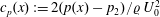 $c_{p}(x):=2(p(x)-p_{2})/\unicode[STIX]{x1D71A}\,U_{0}^{2}$
. As a result, the maximum sheet length is given implicitly as an argument of the pressure distribution with the important condition
$c_{p}(x):=2(p(x)-p_{2})/\unicode[STIX]{x1D71A}\,U_{0}^{2}$
. As a result, the maximum sheet length is given implicitly as an argument of the pressure distribution with the important condition
 $f=1/\unicode[STIX]{x1D70F}(\hat{a})$
:
$f=1/\unicode[STIX]{x1D70F}(\hat{a})$
:
 $$\begin{eqnarray}c_{p}(\hat{a})\approx 1.67\left(\frac{fR_{0}}{U_{0}}\right)^{2}-\unicode[STIX]{x1D70E}.\end{eqnarray}$$
In cases where the conditions
 $Re\rightarrow \infty$
and
$Re\rightarrow \infty$
and
 $We\rightarrow \infty$
are not met, the well-known Rayleigh–Plesset equation or the Keller–Miksis equation has to be solved numerically to calculate the collapse time
$We\rightarrow \infty$
are not met, the well-known Rayleigh–Plesset equation or the Keller–Miksis equation has to be solved numerically to calculate the collapse time
 $\unicode[STIX]{x1D70F}$
.
$\unicode[STIX]{x1D70F}$
.
The nucleation rate
 $f$
together with the initial bubble radius
$f$
together with the initial bubble radius
 $R_{0}$
are the crucial parameters of the model. In the following we present two approaches that show how (3.2) helps to gain insights into the physics of sheet and cloud cavitation.
$R_{0}$
are the crucial parameters of the model. In the following we present two approaches that show how (3.2) helps to gain insights into the physics of sheet and cloud cavitation.
First: equation (3.2) can be used for an order of magnitude estimation of the nucleation rate. In our experiments (Pelz et al.
Reference Pelz, Keil and Ludwig2014) we see that
 $c_{p}(\hat{a})+\unicode[STIX]{x1D70E}$
ranges between 0.29 and 0.66. A typical velocity of the flow is
$c_{p}(\hat{a})+\unicode[STIX]{x1D70E}$
ranges between 0.29 and 0.66. A typical velocity of the flow is
 $U_{0}=10\,\text{m}~\text{s}^{-1}$
. With
$U_{0}=10\,\text{m}~\text{s}^{-1}$
. With
 $c_{p}(\hat{a})+\unicode[STIX]{x1D70E}=0.5$
and the assumption that the detaching bubbles are of the same order of magnitude as the obstacle height,
$c_{p}(\hat{a})+\unicode[STIX]{x1D70E}=0.5$
and the assumption that the detaching bubbles are of the same order of magnitude as the obstacle height,
 $R_{0}\sim \hat{k}=0.5\,\text{mm}$
, we end up with a nucleation rate of
$R_{0}\sim \hat{k}=0.5\,\text{mm}$
, we end up with a nucleation rate of
 $f\approx 11\,\text{kHz}$
which is of the same order of magnitude as the nucleation rates assumed by Hsiao et al. (Reference Hsiao, Ma and Chahine2014), Chahine (Reference Chahine2015) and Ma et al. (Reference Ma, Hsiao and Chahine2015). Of course, the assumption
$f\approx 11\,\text{kHz}$
which is of the same order of magnitude as the nucleation rates assumed by Hsiao et al. (Reference Hsiao, Ma and Chahine2014), Chahine (Reference Chahine2015) and Ma et al. (Reference Ma, Hsiao and Chahine2015). Of course, the assumption
 $R_{0}\sim \hat{k}$
has to be treated with some reservation. As already mentioned
$R_{0}\sim \hat{k}$
has to be treated with some reservation. As already mentioned
 $\hat{k}$
is more likely to be an upper bound for the initial bubble radius
$\hat{k}$
is more likely to be an upper bound for the initial bubble radius
 $R_{0}$
: the experiments conducted by the first and third author of this manuscript indicate that there is a strong dependence of the bubbles radius on the flow parameters (cf. Groß et al.
Reference Groß, Ludwig and Pelz2016).
$R_{0}$
: the experiments conducted by the first and third author of this manuscript indicate that there is a strong dependence of the bubbles radius on the flow parameters (cf. Groß et al.
Reference Groß, Ludwig and Pelz2016).

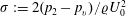
Figure 4. Sheet cavity length
 $a_{+}$
plotted against cavitation number for four Reynolds numbers and three obstacle heights (experimental data by Pelz et al.
Reference Pelz, Keil and Ludwig2014). The solid lines are calculated with (3.2) using the approach
$a_{+}$
plotted against cavitation number for four Reynolds numbers and three obstacle heights (experimental data by Pelz et al.
Reference Pelz, Keil and Ludwig2014). The solid lines are calculated with (3.2) using the approach
 $(fR_{0}/U_{0})^{2}=0.97\,k_{+}^{0.3}$
.
$(fR_{0}/U_{0})^{2}=0.97\,k_{+}^{0.3}$
.
Second: the model can be used to calculate the sheet length and to compare the results with experimental data, see figure 4. With (3.2) it can be concluded that
 $(fR_{0}/U_{0})^{2}$
has to be of the same order of magnitude as the sum of cavitation number
$(fR_{0}/U_{0})^{2}$
has to be of the same order of magnitude as the sum of cavitation number
 $\unicode[STIX]{x1D70E}$
and the pressure distribution
$\unicode[STIX]{x1D70E}$
and the pressure distribution
 $c_{p}$
which is of the order of 0.1–1, as previously mentioned. In general, the nucleation rate
$c_{p}$
which is of the order of 0.1–1, as previously mentioned. In general, the nucleation rate
 $f$
and the size of the detaching free nuclei
$f$
and the size of the detaching free nuclei
 $R_{0}$
depend on surface tension and viscosity, as well as on the size and shape of the nucleation site that is located on the rigid surface. Since nucleation is a mass transfer problem the nucleation rate also depends on the diffusion coefficient
$R_{0}$
depend on surface tension and viscosity, as well as on the size and shape of the nucleation site that is located on the rigid surface. Since nucleation is a mass transfer problem the nucleation rate also depends on the diffusion coefficient
 ${\mathcal{D}}$
, or in dimensionless arguments on the Schmidt number
${\mathcal{D}}$
, or in dimensionless arguments on the Schmidt number
 $Sc:=\unicode[STIX]{x1D708}/{\mathcal{D}}$
, and the supersaturation of the liquid
$Sc:=\unicode[STIX]{x1D708}/{\mathcal{D}}$
, and the supersaturation of the liquid
 $\unicode[STIX]{x1D701}$
. The supersaturation is defined as
$\unicode[STIX]{x1D701}$
. The supersaturation is defined as
 $\unicode[STIX]{x1D701}:=c/c_{N}-1$
, where
$\unicode[STIX]{x1D701}:=c/c_{N}-1$
, where
 $c$
is the measurable concentration of gas in the liquid and
$c$
is the measurable concentration of gas in the liquid and
 $c_{N}$
is the equilibrium saturation concentration at the nucleation site which is determined by the local pressure due to Henry’s law. Physical modelling and experiments indicate that the nucleation rate depends linearly on the supersaturation,
$c_{N}$
is the equilibrium saturation concentration at the nucleation site which is determined by the local pressure due to Henry’s law. Physical modelling and experiments indicate that the nucleation rate depends linearly on the supersaturation,
 $f\propto \unicode[STIX]{x1D701}$
(Groß et al.
Reference Groß, Ludwig and Pelz2016). Thus we obtain
$f\propto \unicode[STIX]{x1D701}$
(Groß et al.
Reference Groß, Ludwig and Pelz2016). Thus we obtain
 $fR_{0}/U_{0}=\unicode[STIX]{x1D701}\,\text{fn}(Re,We,Sc,k_{+})$
. In the experiments the supersaturation has not been measured but it is likely that it only varies within a small range. For a constant supersaturation of the liquid
$fR_{0}/U_{0}=\unicode[STIX]{x1D701}\,\text{fn}(Re,We,Sc,k_{+})$
. In the experiments the supersaturation has not been measured but it is likely that it only varies within a small range. For a constant supersaturation of the liquid
 $\unicode[STIX]{x1D701}\approx \text{const.}$
,
$\unicode[STIX]{x1D701}\approx \text{const.}$
,
 $Re\rightarrow \infty$
,
$Re\rightarrow \infty$
,
 $Sc\rightarrow \infty$
,
$Sc\rightarrow \infty$
,
 $We\rightarrow \infty$
it is reasonable to assume
$We\rightarrow \infty$
it is reasonable to assume
 $fR_{0}/U_{0}$
to be only dependent on the obstacle height
$fR_{0}/U_{0}$
to be only dependent on the obstacle height
 $k_{+}$
in a first step. The investigation of the dependence of the nucleation rate
$k_{+}$
in a first step. The investigation of the dependence of the nucleation rate
 $f$
and the initial bubble radius
$f$
and the initial bubble radius
 $R_{0}$
on the flow parameters is part of current research and not known so far.
$R_{0}$
on the flow parameters is part of current research and not known so far.
Figure 4 shows the dependency of the length of the sheet cavity
 $a_{+}$
on the cavitation number
$a_{+}$
on the cavitation number
 $\unicode[STIX]{x1D70E}$
for different Reynolds numbers
$\unicode[STIX]{x1D70E}$
for different Reynolds numbers
 $Re$
and three obstacle heights
$Re$
and three obstacle heights
 $k_{+}$
. The symbols are experimental data (cf. Pelz et al.
Reference Pelz, Keil and Ludwig2014) and the solid lines represent the results of calculations with (3.2). First of all we want to summarise the main findings of the experiments. The experiments illustrate that: (i) the sheet cavity length
$k_{+}$
. The symbols are experimental data (cf. Pelz et al.
Reference Pelz, Keil and Ludwig2014) and the solid lines represent the results of calculations with (3.2). First of all we want to summarise the main findings of the experiments. The experiments illustrate that: (i) the sheet cavity length
 $a_{+}$
does not depend on the Reynolds number
$a_{+}$
does not depend on the Reynolds number
 $Re$
; (ii) it increases with decreasing cavitation number
$Re$
; (ii) it increases with decreasing cavitation number
 $\unicode[STIX]{x1D70E}$
; and (iii) it increases with increasing obstacle height
$\unicode[STIX]{x1D70E}$
; and (iii) it increases with increasing obstacle height
 $k_{+}$
. Looking at the experimental results one might think that there is a linear dependency
$k_{+}$
. Looking at the experimental results one might think that there is a linear dependency
 $a_{+}=a_{+}(\unicode[STIX]{x1D70E})$
. Since
$a_{+}=a_{+}(\unicode[STIX]{x1D70E})$
. Since
 $c_{p}(a_{+})$
is nonlinear for the examined nozzle, this assumption is unlikely to be true. In addition, for
$c_{p}(a_{+})$
is nonlinear for the examined nozzle, this assumption is unlikely to be true. In addition, for
 $\unicode[STIX]{x1D70E}\rightarrow \infty$
we expect
$\unicode[STIX]{x1D70E}\rightarrow \infty$
we expect
 $a_{+}\rightarrow 0$
which cannot be met by a linear relation. Furthermore it should be mentioned that the sheet length seems to be independent of the obstacle height for small cavitation numbers. In the case of small cavitation numbers, pronounced cloud cavitation complicates the determination of the sheet length. General statements regarding the length of the sheet cavity are reliable only to a limited extent if the sheet cavity is altering its length very fast, i.e. if high cloud detachment frequencies occur. The measured points on the far left (
$a_{+}\rightarrow 0$
which cannot be met by a linear relation. Furthermore it should be mentioned that the sheet length seems to be independent of the obstacle height for small cavitation numbers. In the case of small cavitation numbers, pronounced cloud cavitation complicates the determination of the sheet length. General statements regarding the length of the sheet cavity are reliable only to a limited extent if the sheet cavity is altering its length very fast, i.e. if high cloud detachment frequencies occur. The measured points on the far left (
 $\unicode[STIX]{x1D70E}\approx 0.7$
) demonstrate this uncertainty.
$\unicode[STIX]{x1D70E}\approx 0.7$
) demonstrate this uncertainty.
The solid lines in figure 4 are the results of (3.2) with
 $(fR_{0}/U_{0})^{2}=0.97\,k_{+}^{0.3}$
, which is a result of a parameter variation. In particular, the calculated curves for
$(fR_{0}/U_{0})^{2}=0.97\,k_{+}^{0.3}$
, which is a result of a parameter variation. In particular, the calculated curves for
 $k_{+}=0.05$
and
$k_{+}=0.05$
and
 $k_{+}=0.0375$
match the experimental data quite well, keeping in mind the simplicity of the model. Indeed, the proposed model captures the basic physical content of the phenomenon. The calculated sheet length
$k_{+}=0.0375$
match the experimental data quite well, keeping in mind the simplicity of the model. Indeed, the proposed model captures the basic physical content of the phenomenon. The calculated sheet length
 $a_{+}$
is (i) of course independent of the Reynolds number
$a_{+}$
is (i) of course independent of the Reynolds number
 $Re$
as assumed, (ii) increases with increasing cavitation number
$Re$
as assumed, (ii) increases with increasing cavitation number
 $\unicode[STIX]{x1D70E}$
and (iii) increases with increasing obstacle height
$\unicode[STIX]{x1D70E}$
and (iii) increases with increasing obstacle height
 $k_{+}$
.
$k_{+}$
.
In conclusion, we have two manifestations for the proposed model based on
 $f=1/\unicode[STIX]{x1D70F}$
. The model assumptions are certainly worth discussing: the interaction between bubbles, different bubble sizes, turbulence and pressure fluctuations are all neglected and influence the results to a certain degree. Moreover, the two-way interaction of the sheet cavity with the main flow is not taken into consideration. In particular, the size of the nuclei is an important parameter. In the case of small nuclei (e.g.
$f=1/\unicode[STIX]{x1D70F}$
. The model assumptions are certainly worth discussing: the interaction between bubbles, different bubble sizes, turbulence and pressure fluctuations are all neglected and influence the results to a certain degree. Moreover, the two-way interaction of the sheet cavity with the main flow is not taken into consideration. In particular, the size of the nuclei is an important parameter. In the case of small nuclei (e.g.
 $R_{0}=1\,\unicode[STIX]{x03BC}\text{m}$
) the resulting collapse times are of the order of micro seconds and smaller, which result in high nucleation rates due to (3.2). In these cases it is conceivable that nucleation sites close to each other produce bubbles that are laterally displaced. In this way the required nucleation rates per nucleation site are much lower. The model should be seen as a new picture of sheet cavitation preparing the ground for further investigations. There is no doubt that further experiments are needed to gain a better understanding of the nucleation process.
$R_{0}=1\,\unicode[STIX]{x03BC}\text{m}$
) the resulting collapse times are of the order of micro seconds and smaller, which result in high nucleation rates due to (3.2). In these cases it is conceivable that nucleation sites close to each other produce bubbles that are laterally displaced. In this way the required nucleation rates per nucleation site are much lower. The model should be seen as a new picture of sheet cavitation preparing the ground for further investigations. There is no doubt that further experiments are needed to gain a better understanding of the nucleation process.
4 Re-entrant jet as an upstream spreading thin viscous film
On the one hand, viscosity, hence Reynolds number, influence the dynamics of sheet growth to a minor extend. Only the bubble dynamics is damped by viscous stresses but this is of minor importance: viscosity does not enter the approximation of the collapse time, equation (3.1). On the other hand, the transition from sheet to cloud cavitation is influenced by viscous effects as experiments show (Pelz et al. Reference Pelz, Keil and Ludwig2014). Hence, the viscous effect comes into the picture by means of the re-entrant jet. In fact, the viscous wall shear stress causes the dissipation within the film and the deceleration of the film.

Figure 5. Sketch of a re-entrant jet modelled as a spreading film. The main flow is from left to right while the re-entrant jet flows in the opposite direction. The coordinate
 $x^{\prime }$
starts at the end of the sheet cavity.
$x^{\prime }$
starts at the end of the sheet cavity.
In figure 5 the re-entrant jet is sketched as a spreading film with a distribution of film thickness
 $h(x^{\prime },t)$
with
$h(x^{\prime },t)$
with
 $x^{\prime }=\hat{a}-x$
. The first and main source of rotation is the generation and diffusion of vorticity within the film. The second source of rotation in cavitating flows, i.e. second source of vorticity
$x^{\prime }=\hat{a}-x$
. The first and main source of rotation is the generation and diffusion of vorticity within the film. The second source of rotation in cavitating flows, i.e. second source of vorticity
 $\unicode[STIX]{x1D735}\unicode[STIX]{x1D71A}\times \unicode[STIX]{x1D735}p$
, is of minor importance and is thus not considered in the presented model. Since
$\unicode[STIX]{x1D735}\unicode[STIX]{x1D71A}\times \unicode[STIX]{x1D735}p$
, is of minor importance and is thus not considered in the presented model. Since
 $p=p_{1}=\text{const.}$
along the free streamline the initial condition
$p=p_{1}=\text{const.}$
along the free streamline the initial condition
 $\dot{\unicode[STIX]{x1D709}}(t=0)=U_{0}$
is derived. The second initial condition
$\dot{\unicode[STIX]{x1D709}}(t=0)=U_{0}$
is derived. The second initial condition
 $h(x^{\prime }=0,\,t=0)=h_{0}$
is derived either by a potential flow solution or a momentum balance. As already mentioned, the initial thickness ranges between 15 % and 35 % of the cavity thickness (Michel Reference Michel1978; Callenaere et al.
Reference Callenaere, Franc, Michel and Riondet2001).
$h(x^{\prime }=0,\,t=0)=h_{0}$
is derived either by a potential flow solution or a momentum balance. As already mentioned, the initial thickness ranges between 15 % and 35 % of the cavity thickness (Michel Reference Michel1978; Callenaere et al.
Reference Callenaere, Franc, Michel and Riondet2001).
It is assumed that the liquid film starts to evolve upstream when the growth of the sheet cavity stagnates. The initial conditions are the initial film velocity
 $\dot{\unicode[STIX]{x1D709}}_{0}$
and the initial height of the liquid film
$\dot{\unicode[STIX]{x1D709}}_{0}$
and the initial height of the liquid film
 $h_{0}$
. The pressure in the liquid film is predetermined by the pressure in the sheet cavity which is approximately equal to
$h_{0}$
. The pressure in the liquid film is predetermined by the pressure in the sheet cavity which is approximately equal to
 $p_{1}$
. The continuity equation for the spreading film, cf. figure 5, can be written in an integral form as
$p_{1}$
. The continuity equation for the spreading film, cf. figure 5, can be written in an integral form as
 $$\begin{eqnarray}\int _{0}^{x^{\prime }}\frac{\unicode[STIX]{x2202}h}{\unicode[STIX]{x2202}t}\,\text{d}x^{\prime }-Q_{0}+Q=0.\end{eqnarray}$$
The volume flow
 $Q_{0}=U_{0}\,h_{0}$
is prescribed as a boundary condition whereas
$Q_{0}=U_{0}\,h_{0}$
is prescribed as a boundary condition whereas
 $Q=Uh$
is unknown.
$Q=Uh$
is unknown.
 $U$
and
$U$
and
 $U_{0}$
are the mean velocities within the film. This equation is equivalent to
$U_{0}$
are the mean velocities within the film. This equation is equivalent to
 $$\begin{eqnarray}\frac{\unicode[STIX]{x2202}h}{\unicode[STIX]{x2202}t}+\frac{\unicode[STIX]{x2202}Q}{\unicode[STIX]{x2202}x^{\prime }}=0\quad \text{or}\quad \frac{\text{D}Q}{\text{D}t}=\frac{Q}{U}\frac{\unicode[STIX]{x2202}U}{\unicode[STIX]{x2202}t}\end{eqnarray}$$
for the sketched infinitesimal control volume. The momentum balance in the streamwise direction gives
 $$\begin{eqnarray}\int _{0}^{x^{\prime }}\frac{\unicode[STIX]{x2202}(Uh)}{\unicode[STIX]{x2202}t}\,\text{d}x^{\prime }-Q_{0}U_{0}+QU=-\int _{0}^{x^{\prime }}\frac{\unicode[STIX]{x1D70F}_{w}}{\unicode[STIX]{x1D71A}}\,\text{d}x^{\prime }.\end{eqnarray}$$
With the local wall friction coefficient defined by
 $c_{f}=2\unicode[STIX]{x1D70F}_{w}/(\unicode[STIX]{x1D71A}\,U_{0}^{2})$
this yields
$c_{f}=2\unicode[STIX]{x1D70F}_{w}/(\unicode[STIX]{x1D71A}\,U_{0}^{2})$
this yields
 $$\begin{eqnarray}\frac{\text{D}Q}{\text{D}t}+Q\frac{\unicode[STIX]{x2202}U}{\unicode[STIX]{x2202}x^{\prime }}=-\frac{U^{2}}{2}c_{f}.\end{eqnarray}$$
The local friction coefficient
 $c_{f}(k_{+},Re)$
is a function of the surface roughness and the local Reynolds number. Inserting the continuity equation into the momentum balance gives the expected result:
$c_{f}(k_{+},Re)$
is a function of the surface roughness and the local Reynolds number. Inserting the continuity equation into the momentum balance gives the expected result:
 $$\begin{eqnarray}\frac{\text{D}U}{\text{D}t}=\frac{U^{2}}{2}\frac{c_{f}}{h}\quad \text{or}\quad \frac{\unicode[STIX]{x2202}U}{\unicode[STIX]{x2202}t}+U\frac{\unicode[STIX]{x2202}U}{\unicode[STIX]{x2202}x^{\prime }}=\frac{U^{2}}{2}\frac{c_{f}}{h}.\end{eqnarray}$$
As one can see, the pressure does not appear in the momentum balance. The pressure in the film is determined by the pressure in the sheet cavity which is approximately
 $p_{1}$
. This conclusion is based on the continuity of the stress vector. Nevertheless, the pressure plays an important role. The pressure distribution which is given by
$p_{1}$
. This conclusion is based on the continuity of the stress vector. Nevertheless, the pressure plays an important role. The pressure distribution which is given by
 $c_{p}$
is of importance for length and height of the sheet cavity as Callenaere et al. (Reference Callenaere, Franc, Michel and Riondet2001) showed. Thus, the pressure gradient influences our results indirectly without being part of the model itself.
$c_{p}$
is of importance for length and height of the sheet cavity as Callenaere et al. (Reference Callenaere, Franc, Michel and Riondet2001) showed. Thus, the pressure gradient influences our results indirectly without being part of the model itself.
Integrating (4.5) from
 $x^{\prime }=0$
to
$x^{\prime }=0$
to
 $x^{\prime }=\unicode[STIX]{x1D709}$
gives
$x^{\prime }=\unicode[STIX]{x1D709}$
gives
 $$\begin{eqnarray}\int _{0}^{\unicode[STIX]{x1D709}}\frac{\unicode[STIX]{x2202}U}{\unicode[STIX]{x2202}t}\,\text{d}x^{\prime }+\frac{\dot{\unicode[STIX]{x1D709}}^{2}}{2}-\frac{U_{0}^{2}}{2}=-\int _{0}^{\unicode[STIX]{x1D709}}\frac{c_{f}}{2}\frac{U}{h}\,\text{d}x^{\prime }.\end{eqnarray}$$
The equation is nothing other than Bernoulli‘s equation. Together with the continuity equation
 $$\begin{eqnarray}\int _{0}^{\unicode[STIX]{x1D709}}\frac{\unicode[STIX]{x2202}h}{\unicode[STIX]{x2202}t}\,\text{d}x^{\prime }-U_{0}\,h_{0}+\dot{\unicode[STIX]{x1D709}}\,h_{\unicode[STIX]{x1D709}}=0\end{eqnarray}$$
we have two equations to be solved simultaneously. To solve this system of equations we follow the linear ansatz with
 $U\approx U_{0}+(\dot{\unicode[STIX]{x1D709}}-U_{0})\,x^{\prime }/\unicode[STIX]{x1D709}$
and
$U\approx U_{0}+(\dot{\unicode[STIX]{x1D709}}-U_{0})\,x^{\prime }/\unicode[STIX]{x1D709}$
and
 $h\approx h_{0}+(h_{\unicode[STIX]{x1D709}}-h_{0})\,x^{\prime }/\unicode[STIX]{x1D709}$
. With the approximations
$h\approx h_{0}+(h_{\unicode[STIX]{x1D709}}-h_{0})\,x^{\prime }/\unicode[STIX]{x1D709}$
. With the approximations
 $$\begin{eqnarray}\displaystyle & \displaystyle \frac{\unicode[STIX]{x2202}U}{\unicode[STIX]{x2202}t}\approx \frac{x^{\prime }}{\unicode[STIX]{x1D709}}\left[\ddot{\unicode[STIX]{x1D709}}-\left(\dot{\unicode[STIX]{x1D709}}-U_{0}\right)\frac{\dot{\unicode[STIX]{x1D709}}}{\unicode[STIX]{x1D709}}\right], & \displaystyle\end{eqnarray}$$
 $$\begin{eqnarray}\displaystyle & \displaystyle \frac{\unicode[STIX]{x2202}h}{\unicode[STIX]{x2202}t}\approx \frac{x^{\prime }}{\unicode[STIX]{x1D709}}\left[{\dot{h}}_{\unicode[STIX]{x1D709}}-\left(h_{\unicode[STIX]{x1D709}}-h_{0}\right)\frac{\dot{\unicode[STIX]{x1D709}}}{\unicode[STIX]{x1D709}}\right]~\text{and} & \displaystyle\end{eqnarray}$$
 $$\begin{eqnarray}\displaystyle & \displaystyle \frac{U^{2}}{2}\frac{c_{f}}{h}\approx R=\text{const.} & \displaystyle\end{eqnarray}$$
the system of equations with the ‘excitation’ on the right-hand side reads:
 $$\begin{eqnarray}\displaystyle & \displaystyle \frac{1}{2}\unicode[STIX]{x1D709}\left[\ddot{\unicode[STIX]{x1D709}}-\left(\dot{\unicode[STIX]{x1D709}}-U_{0}\right)\frac{\dot{\unicode[STIX]{x1D709}}}{\unicode[STIX]{x1D709}}\right]+\frac{\dot{\unicode[STIX]{x1D709}}^{2}}{2}+R\,\unicode[STIX]{x1D709}=\frac{U_{0}^{2}}{2}, & \displaystyle\end{eqnarray}$$
 $$\begin{eqnarray}\displaystyle & \displaystyle \frac{1}{2}\unicode[STIX]{x1D709}\left[{\dot{h}}_{\unicode[STIX]{x1D709}}-\left(h_{\unicode[STIX]{x1D709}}-h_{0}\right)\frac{\dot{\unicode[STIX]{x1D709}}}{\unicode[STIX]{x1D709}}\right]-U_{0}\,h_{0}+\dot{\unicode[STIX]{x1D709}}\,h_{\unicode[STIX]{x1D709}}=0. & \displaystyle\end{eqnarray}$$
This system of equations in the unknowns
 $\unicode[STIX]{x1D709}(t)$
and
$\unicode[STIX]{x1D709}(t)$
and
 $h_{\unicode[STIX]{x1D709}}(t)$
with the three initial conditions
$h_{\unicode[STIX]{x1D709}}(t)$
with the three initial conditions
 $\unicode[STIX]{x1D709}(0)=0,\,\dot{\unicode[STIX]{x1D709}}(0)=U_{0}$
and
$\unicode[STIX]{x1D709}(0)=0,\,\dot{\unicode[STIX]{x1D709}}(0)=U_{0}$
and
 $h_{\unicode[STIX]{x1D709}}(0)=h_{0}$
has to be solved numerically and allows for the calculation of the position and the velocity of the liquid film and its height.
$h_{\unicode[STIX]{x1D709}}(0)=h_{0}$
has to be solved numerically and allows for the calculation of the position and the velocity of the liquid film and its height.
The question is whether the liquid film will reach the point of origin or not. In the first case we see cloud cavitation. To calculate the behaviour of the liquid film we assume that the initial height of the liquid film in general is 15 % of the average height of the sheet cavity (cf. Callenaere et al. Reference Callenaere, Franc, Michel and Riondet2001). The friction coefficient is modelled as a turbulent flow above a plate. We use
 $$\begin{eqnarray}R=\frac{U_{0}^{2}}{2}\frac{c_{f}}{h_{0}}\end{eqnarray}$$
and
 $$\begin{eqnarray}c_{f}=2\left[\frac{\unicode[STIX]{x1D705}}{\ln Re_{J}}\,G(\ln Re_{J})\right]^{2},\end{eqnarray}$$
with the von Kármán constant
 $\unicode[STIX]{x1D705}=0.41$
, the Reynolds number of the film defined by
$\unicode[STIX]{x1D705}=0.41$
, the Reynolds number of the film defined by
 $Re_{J}=U_{0}\,h_{0}/\unicode[STIX]{x1D708}$
and coefficient
$Re_{J}=U_{0}\,h_{0}/\unicode[STIX]{x1D708}$
and coefficient
 $G=1.5$
for
$G=1.5$
for
 $10^{5}<Re_{J}<10^{6}$
to model the friction (cf. Schlichting & Gersten Reference Schlichting and Gersten2006).
$10^{5}<Re_{J}<10^{6}$
to model the friction (cf. Schlichting & Gersten Reference Schlichting and Gersten2006).

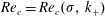
Figure 6. Stability map for sheet and cloud cavitation for
 $k_{+}=0.025$
. The map shows operation points where sheet (squares) and cloud cavitation (circles) occur. Operation points marked with diamonds could not be categorised. The larger symbols mark the experimental data, the smaller symbols are the results of the physical model (experimental data by Pelz et al.
Reference Pelz, Keil and Ludwig2014).
$k_{+}=0.025$
. The map shows operation points where sheet (squares) and cloud cavitation (circles) occur. Operation points marked with diamonds could not be categorised. The larger symbols mark the experimental data, the smaller symbols are the results of the physical model (experimental data by Pelz et al.
Reference Pelz, Keil and Ludwig2014).

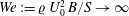
Figure 7. Stability map for sheet and cloud cavitation for
 $k_{+}=0.0375$
. The map shows operation points where sheet (squares) and cloud cavitation (circles) occur. Operation points marked with diamonds could not be categorised. The larger symbols mark the experimental data, the smaller symbols are the results of the physical model (experimental data by Pelz et al.
Reference Pelz, Keil and Ludwig2014).
$k_{+}=0.0375$
. The map shows operation points where sheet (squares) and cloud cavitation (circles) occur. Operation points marked with diamonds could not be categorised. The larger symbols mark the experimental data, the smaller symbols are the results of the physical model (experimental data by Pelz et al.
Reference Pelz, Keil and Ludwig2014).

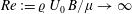
Figure 8. Stability map for sheet and cloud cavitation for
 $k_{+}=0.05$
. The map shows operation points where sheet (squares) and cloud cavitation (circles) occur. Operation points marked with diamonds could not be categorised. The larger symbols mark the experimental data, the smaller symbols are the results of the physical model (experimental data by Pelz et al.
Reference Pelz, Keil and Ludwig2014).
$k_{+}=0.05$
. The map shows operation points where sheet (squares) and cloud cavitation (circles) occur. Operation points marked with diamonds could not be categorised. The larger symbols mark the experimental data, the smaller symbols are the results of the physical model (experimental data by Pelz et al.
Reference Pelz, Keil and Ludwig2014).
For constant
 $R$
the asymptotic solution with
$R$
the asymptotic solution with
 $\dot{\unicode[STIX]{x1D709}}=0$
and
$\dot{\unicode[STIX]{x1D709}}=0$
and
 $\ddot{\unicode[STIX]{x1D709}}=0$
of (4.11) is
$\ddot{\unicode[STIX]{x1D709}}=0$
of (4.11) is
 $\hat{\unicode[STIX]{x1D709}}=U_{0}^{2}/2R=h_{0}/c_{f}$
. A comparison of the calculated maximum length of the liquid film with the measured sheet length gives the answer to the question above. For
$\hat{\unicode[STIX]{x1D709}}=U_{0}^{2}/2R=h_{0}/c_{f}$
. A comparison of the calculated maximum length of the liquid film with the measured sheet length gives the answer to the question above. For
 $\hat{\unicode[STIX]{x1D709}}\geqslant \hat{a}$
the operation point is classified as cloud cavitation, for
$\hat{\unicode[STIX]{x1D709}}\geqslant \hat{a}$
the operation point is classified as cloud cavitation, for
 $\hat{\unicode[STIX]{x1D709}}<\hat{a}$
it is classified as sheet cavitation. One has to mention that it is possible to calculate a larger penetration length of the re-entrant jet than the actual length of the sheet cavity,
$\hat{\unicode[STIX]{x1D709}}<\hat{a}$
it is classified as sheet cavitation. One has to mention that it is possible to calculate a larger penetration length of the re-entrant jet than the actual length of the sheet cavity,
 $\hat{\unicode[STIX]{x1D709}}>\hat{a}$
. This is only a result of the differential equation but of course cannot be seen in the experiments. In these cases the re-entrant jet could flow upstream much further.
$\hat{\unicode[STIX]{x1D709}}>\hat{a}$
. This is only a result of the differential equation but of course cannot be seen in the experiments. In these cases the re-entrant jet could flow upstream much further.
By plotting Reynolds number against cavitation number and using different symbols to mark the two cavitation regimes we obtain stability maps for different heights of the artificial roughness, figures 6–8. Every symbol in the diagrams marks one operation point that has been measured, evaluated and analysed. Operation points where sheet cavitation (squares) and cloud cavitation (circles) occur can be identified. Operation points marked with diamonds could not be categorised and are interpreted as a transition area. The larger symbols mark the experimental data, the smaller symbols are the results of the physical model.
The stability maps show that there are two possible ways to avoid operation points in which cloud cavitation occur. The first way is to increase the cavitation number which is the most common procedure. The other possible way is to decrease the Reynolds number. One can see that for small Reynolds numbers no cloud cavitation exists. In these cases the film does not reach the artificial roughness since
 $\hat{\unicode[STIX]{x1D709}}<\hat{a}$
. The stagnation pressure
$\hat{\unicode[STIX]{x1D709}}<\hat{a}$
. The stagnation pressure
 $\unicode[STIX]{x1D71A}U_{0}^{2}/2$
that drives the film flow is too small. The graphs show that the transition from sheet to cloud cavitation can be predicted remarkably well by the presented model.
$\unicode[STIX]{x1D71A}U_{0}^{2}/2$
that drives the film flow is too small. The graphs show that the transition from sheet to cloud cavitation can be predicted remarkably well by the presented model.
An application of our model to real hydraulic devices is difficult because of the complex flow conditions. Nevertheless the findings could be used to tackle problems of technical relevance. If a hydraulic device (pump, turbine, propeller, etc.) is usually operated in operation points where cloud cavitation occurs it would be worth considering increasing the surface roughness in the region where the re-entrant jet develops. Kawanami et al. (Reference Kawanami, Kato, Yamaguchi, Tanimura and Tagaya1997) showed that a small obstacle placed in that region can stop the re-entrant jet. Callenaere et al. (Reference Callenaere, Franc, Michel and Riondet2001) suspected that smaller wall surface perturbations, such as distributed roughness, influence the cloud cavitation instability. Our interpretation of the re-entrant jet as a viscous film supports this hypothesis and provides an explanation. To fully understand the phenomenon of cloud cavitation one has to consider the interaction of the re-entrant jet with the solid wall as we addressed in this paper.
5 Conclusion
For engineers and operators dealing with cavitation in hydraulic components such as pumps, turbines, propellers or valves it is important to know that there are various kinds of cavitation regimes which differ in appearance and erosive potential. Failures of hydraulic components due to cavitation are often caused by a lack of knowledge about the different cavitation regimes and their erosive potential. Therefore the prediction of critical operating parameters is of great value to identify harmful operation points already in the design process or during the operation of technical applications.
In the present paper we investigate sheet and cloud cavitation and the transition between these two regimes, which depends on cavitation number and Reynolds number. It is of practical importance to understand and predict this transition, since sheet cavitation is in general harmless whereas cloud cavitation has a high potential to damage material and to cause noise and vibration.
For this purpose we present an analytical model that describes the two main mechanisms: the growth of the sheet cavity and the flow of the re-entrant jet. The asymptotic sheet growth model allows for the calculation of the length of the sheet cavity for a given nucleation rate or vice versa. The flow of the re-entrant jet is interpreted as a viscous film that streams upstream beneath the sheet cavity. The film theory allows to consider viscous effects and thus an influence of the Reynolds number. The transition from sheet to cloud cavitation occurs if the liquid film reaches the point of origin of the sheet cavity, or in other words if the length of the viscous film is equal to the length of the sheet cavity.
Although the models do not include the interaction between bubbles, the interaction of the sheet cavity with the main flow and other effects, such as turbulence and pressure fluctuations, the results fit remarkably well to experimental data and help to gain new insights into the physics of this complex phenomenon.
Acknowledgement
The presented results were obtained within the research project no. 16054 N/1, funded by budget resources of the Bundesministerium für Wirtschaft und Technologie (BMWi) approved by the Arbeitsgemeinschaft industrieller Forschungsvereinigungen ‘Otto von Guericke’ e.V. (AiF).


 Open access