


1. Introduction
The dynamics in the airflow above wind-generated waves is crucial for wind–wave coupling and for the air–sea momentum flux as a whole (Janssen Reference Janssen1989; Komen et al. Reference Komen, Cavaleri, Donelan, Hasselmann, Hasselmann and Janssen1994; Belcher & Hunt Reference Belcher and Hunt1998; Edson & Fairal Reference Edson and Fairal1998; Janssen Reference Janssen1999; Sullivan & McWilliams Reference Sullivan and McWilliams2002; Sullivan et al. Reference Sullivan, Edson, Hristov and McWilliams2008; Mueller & Veron Reference Mueller and Veron2009; Sullivan & McWilliams Reference Sullivan and McWilliams2010; Grare, Lenain & Melville Reference Grare, Lenain and Melville2013a; Suzuki, Hara & Sullivan Reference Suzuki, Hara and Sullivan2013; Hara & Sullivan Reference Hara and Sullivan2015; Grare, Lenain & Melville Reference Grare, Lenain and Melville2018). Detailed experimental investigations of the airflow structure and wind stress above wind waves remain rare, however, largely because of the technical challenges involved with acquiring high resolution measurements very close to a rapidly moving interface (Buckley & Veron Reference Buckley and Veron2017). Yet, it is now accepted that surface waves in general, and airflow separation and wave breaking processes in particular, play an important role in the momentum flux between the ocean and the atmosphere (Melville Reference Melville1996; Sullivan & McWilliams Reference Sullivan and McWilliams2010). Thus, there is a need for detailed airflow and surface stress measurements above wind waves. This is particularly true in high wind conditions where momentum flux parametrizations still need to be improved in order to help better predict extreme weather events such as tropical storms (e.g. Edson et al. Reference Edson, Jampana, Weller, Bigorre, Plueddemann, Fairall, Miller, Mahrt, Vickers and Hersbach2013; Veron Reference Veron2015).
At moderate to high wind speeds, and/or when waves break, airflow separation is believed to have an important impact on the total air–sea momentum flux. However, our current understanding of airflow separation over wind waves is still rather poor and detailed measurements are lacking. Consequently, the effects of airflow separation on the surface stress and the range of wind speeds over which separation substantially affects the air–sea momentum flux are not well resolved.
Airflow separation began receiving increased interest over four decades ago, when Banner & Melville (Reference Banner and Melville1976) conducted flow-visualization studies and established on theoretical grounds derived from the earlier work of Banner & Phillips (Reference Banner and Phillips1974), that airflow separation over a surface gravity wave occurs concurrently with breaking (see also the work of Gent & Taylor Reference Gent and Taylor1977). A year later, Okuda, Kawai & Toba (Reference Okuda, Kawai and Toba1977) quantified the surface stress over wind waves at relatively short fetches (2.85 m) and noted that the dominant mechanism for transferring energy from the air to the water was the high tangential stress at the interface. This was in contrast with the results of Banner & Melville (Reference Banner and Melville1976), who found that the normal, not tangential stress, was the main contributor to the momentum flux between air and water. Neither study discussed the instantaneous turbulent structures present when the airflow separates. In order to fill this gap, Kawai (Reference Kawai1981, Reference Kawai1982) performed a qualitative flow visualization study over short wind waves and was able to detect the separated airflow. He suggested that airflow separation was caused by the inability of the airflow to curve along the steep slope of the wave crest. Later, Kawamura & Toba (Reference Kawamura and Toba1988) performed instantaneous velocity-shear measurements in the separated flow over wind waves using a pair of surface following hot-films. They explained the abrupt change in the velocity across an observed shear layer by the existence of a separation region behind the wind-wave crest. Reul, Branger & Giovanangeli (Reference Reul, Branger and Giovanangeli1999) pioneered the use of PIV (particle image velocimetry) in the airflow over waves and quantified airflow separation over mechanically generated breaking waves. They reported the presence of multiple coherent patches of vorticity downwind of the crest that were strongly influenced by the geometry of the breaker (see also Reul, Branger & Giovanangeli Reference Reul, Branger and Giovanangeli2008). More recently, Veron, Saxena & Misra (Reference Veron, Saxena and Misra2007) were able to identify airflow separation events over wind-generated waves. Later, Buckley & Veron (Reference Buckley and Veron2016) and Buckley & Veron (Reference Buckley and Veron2017) determined that separation dramatically enhances the along-wave turbulent stress and kinetic energy distributions past the crest of the average wind wave. Subsequent analysis is also presented in Buckley & Veron (Reference Buckley and Veron2019), Husain et al. (Reference Husain, Hara, Buckley, Yousefi, Veron and Sullivan2019) and Yousefi, Veron & Buckley (Reference Yousefi, Veron and Buckley2020). Finally, two important laboratory studies that focused on estimating the near-surface viscous stress at the wavy air–water interface should be mentioned here. First, Banner & Peirson (Reference Banner and Peirson1998), using underwater PIV measurements under wind-generated waves, estimated along-wave near-surface tangential stresses. Grare et al. (Reference Grare, Peirson, Branger, Walker, Giovanangeli and Makin2013b) were able to estimate near-surface viscous stresses very close to the surface by plunging a hot-wire anemometer into the wavy water. In both of these studies, however, a quantification of airflow separation effects was not possible.
Coincidentally, a number of direct numerical simulation (DNS) and large eddy simulation (LES) investigations of the airflow and airflow separation above solid wavy surfaces were initiated (Kuzan, Hanratty & Adrian Reference Kuzan, Hanratty and Adrian1989; Maass & Schumann Reference Maass and Schumann1994; Gong, Taylor & Dornbrack Reference Gong, Taylor and Dornbrack1996; Angelis, Lombardi & Banerjee Reference Angelis, Lombardi and Banerjee1997; Henn & Sykes Reference Henn and Sykes1999). In particular, Maass & Schumann (Reference Maass and Schumann1994) and Calhoun & Street (Reference Calhoun and Street2001) studied the turbulent flow near the wavy wall and confirmed that a wavy surface substantially modifies classical wall turbulence. They also provided some insight into the detailed three-dimensional instantaneous structures in the separated region. Later, Sullivan, McWilliams & Moeng (Reference Sullivan, McWilliams and Moeng2000) and Shen et al. (Reference Shen, Zhang, Yue and Triantafyllou2003) modelled the airflow over a moving sinusoidal wall. In recent years, LES and DNS simulations have considerably improved and allowed for increasing complexity to be accounted for. In particular, multi-modal surface geometry and propagating surface waves can now be incorporated in the simulation with good success (Yang & Shen Reference Yang and Shen2010; Sullivan, McWilliams & Patton Reference Sullivan, McWilliams and Patton2014; Hara & Sullivan Reference Hara and Sullivan2015; Sullivan et al. Reference Sullivan, Banner, Morison and Peirson2018; Wang et al. Reference Wang, Zhang, Hao, Huang, Shen, Xu and Zhang2020) but available experimental data to validate these simulations are lacking.
In this paper, we present two-dimensional high resolution measurements of the airflow above wind-generated waves, within the airflow's viscous sublayer and above. We further investigate the mean and phase-averaged contributions of viscous stress to the total momentum flux across the air–water interface and the energy flux contributing to wind-wave growth. Finally, the impact of airflow separation on the average surface viscous stress is discussed.
2. Experimental set-up and methods
The experiments presented in this paper were performed in the University of Delaware's large wind-wave-current facility. The tank, specially designed for the study of air–sea interactions, is 42 m long, 1 m wide and 1.25 m high. The mean water depth was kept at 0.70 m, with an airflow space of 0.55 m. For this study, wind waves were generated by the computer-controlled recirculating wind tunnel, sketched in figure 1(a). In this paper, we present results for six different wind/wave conditions. Winds were generated with mean 10 m equivalent speeds of  $U_{10} = 0.86$, 2.19, 5.00, 9.41, 14.34 and $16.63\ \textrm {m}\ \textrm {s}^{-1}$. The data were collected at a fetch of 22.7 m. The different experimental conditions are summarized in table 1.

Figure 1. Sketch of University of Delaware's large wind-wave tank (a). The experimental set-up is positioned at a fetch of 22.7 m. Upwind view of the imaging system (b). The optical paths of the pulsed Nd-Yag laser sheets are shown. Velocities in the airflow are measured by PIV, and wave properties are measured by laser-induced fluorescence (LIF). LIF systems include the PIVSD camera (for water surface detection on PIV images), the large field of view (LFV) laser and camera (for large field of view snapshots of wave profiles) and optical wave gauge (WG) cameras.
Table 1. Summary of the experimental conditions. Measured, apparent peak wave frequencies  $f_m$ were obtained from the optical wave gauge frequency spectra. The wave speed $c$ denotes the intrinsic phase speed and was extracted using a cross-spectral analysis of two consecutive optical wave gauge signals which included the wind-induced drift $u_d$. The wave amplitude $a$ is estimated using $a=\sqrt {2}a_{rms}$, where $a_{rms}$ is the root-mean-squared amplitude measured with optical wave gauges. The wall-normalized roughness length (or roughness Reynolds number, Donelan Reference Donelan1998) is given by $z_{0}^+ = u_* z_0 / \nu$ (where $z_0$ is the roughness length and $\nu$ the air kinematic viscosity). Both $u_*$ and $z_0$ are estimated from the mean velocity profiles assuming classical log behaviour outside the wave boundary layer. $U_{10}$ is the mean air velocity extrapolated from the measurements to $z = 10$ m, obtained by fitting the upper logarithmic part of each mean velocity profile. $\delta _{\nu } k$ is the thickness of the viscous sublayer scaled by wavenumber $k$, with $\delta _{\nu } = 10 \nu / u_*$ (e.g. Phillips Reference Phillips1977, p. 128).

A complex imaging system was developed for the study of the airflow above wind waves. The experimental set-up, combining PIV with LIF techniques, allowed us to simultaneously obtain two-dimensional velocity fields in the air above the wind-generated waves, together with spatial and temporal wave properties. The apparatus and data processing techniques are described in detail in Buckley & Veron (Reference Buckley and Veron2017). Accordingly, we will present below a brief summarized overview of the complete system.
2.1. Airflow velocity measurements
In order to obtain high resolution, two-dimensional velocity measurements in the airflow above surface wind waves, we used a custom built PIV–LIF system. For this, the airflow was seeded with 8 to  $12\ \mathrm {\mu }\textrm {m}$ water droplets generated by a commercial fog generator and illuminated with a high intensity pulsed green laser light sheet (Nd-Yag, $200\ \textrm {mJ}\ \textrm {pulse}^{-1}$, 3–5 ns pulse duration). The light sheet was aligned in the along-wind direction and positioned in the centre line of the tank (see figure 1). Sequential image pairs of the seeded flow were obtained with two side-by-side CCD cameras (JAI, $2048 \times 2048$ pixel). The adjacent PIV images were merged together in order to obtain a high resolution ( $47\ \mathrm {\mu }\textrm {m}\ \textrm {pixel}^{-1}$) $18.7\ \textrm {cm}\times 9.7\ \textrm {cm}$ PIV image. The resulting PIV image pairs were then processed using conventional cross-correlation techniques (Raffel et al. Reference Raffel, Willert, Wereley and Kompenhans2007) performed using an in-house iterative multi-grid software. Two-dimensional velocity maps were thus obtained with a velocity vector measurement every $188\ \mathrm {\mu }\textrm {m}^2$ over the $18.7\ \textrm {cm}\times 9.7\ \textrm {cm}$ imaging footprint. The PIV cameras operated at 14.4 frames/second yielding PIV velocity maps at a 7.2 Hz rate. Low laser light reflection from the air–water interface rendered precise automated surface detection difficult on the raw PIV images. To address this issue, high resolution ( $100\ \mathrm {\mu }\textrm {m}\ \textrm {pixel}^{-1}$) LIF images (PIV surface detection images, noted ‘PIVSD’) of the wave surface profiles within the PIV field of view were acquired simultaneously with the PIV images. This was achieved by adding a liquid solution of Rhodamine 6G dye to the water at a concentration of $8 \times 10^{-6}\ \textrm {g}\ \textrm {L}^{-1}$. The fluorescent dye was then excited by the PIV laser and images of the surface were collected with a CCD camera identical to those used for the PIV. An optical filter was also used to remove green laser light reflections (and potential contamination from light scattered by the fog particles), and isolate the light emitted by the fluorescent dye. This yielded sharp, crisp images of the interface which was then automatically detected using an in-house, gradient-based edge-detection image processing software (as pioneered by Duncan (Reference Duncan1981), Duncan et al. (Reference Duncan, Qiao, Philomin and Wenz1999), for the study of mechanically generated waves). In turn, being able to properly locate the air–water interface on the PIV images allowed us to perform velocity measurements very close to the interface. In the end, airflow velocities were consistently measured as close as
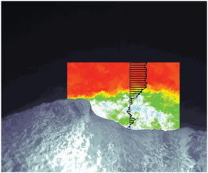
  $100\ \mathrm {\mu }\textrm {m}$ above the air–water interface. A sample merged PIV–PIVSD image is plotted in figure 2.

Figure 2. A composite image showing the air-side portion of merged raw PIV images, plotted above the water-side portion of the PIVSD image used for surface detection. The background image is the LFV LIF. WG fields of view are also displayed, up and downwind of the PIV field of view. This sextuplet of instantaneous PIV–LIF images was acquired during the experiment with  $U_{10}=5.00\ \textrm {m}\ \textrm {s}^{-1}$.
2.2. Wind-wave measurements
The LIF technique employed to precisely locate the air–water interface within the PIV frame was also used to measure two additional types of wind wave data: along-channel spatial surface profiles with high spatial resolution, and single point high frequency wave height measurements.
Large along-channel spatial profiles of the wavy surface were obtained by LIF, using a third CCD camera (JAI,  $2048\times 2048$ pixel, noted ‘LFV’ hereafter), that was focused on the intersection with the surface of a long green laser sheet, generated by a second pulsed Nd-Yag laser ( $120\ \textrm {mJ}\ \textrm {pulse}^{-1}$, 3–5 ns pulse duration). The resulting LFV images provided measurements of the along-channel surface elevation in the centre line of the channel over a length of $51.2\ \textrm {cm}$ $(0.25\ \textrm {mm}\ \textrm {pixel}^{-1}\ \text {resolution})$, and at a rate of 7.2 Hz. The LFV field of view was positioned in the same along-channel plane as the PIV images, and extended 16.7 cm upwind and 15.8 cm downwind of the PIV field of view (figure 2).
Finally, four single point optical wave gauges, provided time series of the water height 2.8 and 1.4 cm upwind and 2.7 and 4.2 cm downwind of the PIV airflow velocity measurements. The system consisted of two CCD cameras (JAI,  $300\times 1600$ pixel), which imaged the intersection with the surface of pairs of 200 mW continuous green laser beams. The resulting LIF images provided measurements of the water height with a resolution of $65 \ \mathrm {\mu }\textrm {m}\ \textrm {pixel}^{-1}$, and at a frequency of 93.6 Hz (figure 2). Peak apparent wave frequencies $f_m$ were obtained from the optical wave gauge frequency spectra. Here, the peak frequencies are Doppler shifted by the wind-induced drift
 \begin{equation} \omega_m = \sigma + k u_d = k (c + u_d), \end{equation}
where  $\omega _m=2 {\rm \pi}f_m$ is the apparent (measured) angular frequency, $c$ and $\sigma$ are the intrinsic phase speed and angular frequency respectively and $k$ is the wavenumber (e.g. Phillips Reference Phillips1977, p. 24). Peak wave speeds $c_m=c+u_d$ were directly estimated using a cross-spectral analysis on two adjacent optical wave gauge signals. The wavenumber $k$ was then readily obtained using (2.1). Next, the intrinsic frequency $\sigma$ and wave phase speed $c$ were estimated using the linear dispersion relationship for deep water gravity waves $\sigma = c k =\sqrt {gk+\varGamma k^3}$ where $\varGamma$ is the surface tension. The wind drift velocity $u_d$ is given by $u_d=({\omega _m-\sigma })/{k}$. Note that the Doppler shifting results from a drift current that acts not only on the surface characteristics of the waves, but also on the underwater wave orbital motions. This means that $u_d$ is an integrated measure of the wind-induced shear currents down to a depth of $O(0.1\lambda )$ (e.g. Stewart & Joy Reference Stewart and Joy1974), rather than a solely surface wind drift velocity $u_s$ (see also Smeltzer et al. Reference Smeltzer, Æsøy, Ådnøy and Ellingsen2019). The peak wave amplitude $a$ was estimated using $a=\sqrt {2}a_{rms}$, where $a_{rms}$ is the root-mean-squared amplitude measured with optical wave gauges (see table 1).
2.3. Experimental procedure
All cameras and pulsed lasers were synchronized using triggers from a single timing computer equipped with National Instruments digital and analogue signal generation software and hardware (see Buckley & Veron (Reference Buckley and Veron2017), for additional details). The wind blower was controlled by an analogue signal, also generated by the timing computer. Each wind-wave experiment followed a fully automated, repeatable procedure. At first, the wind was slowly increased to its target steady value. After the wave field had sufficiently developed and reached a fetch-limited equilibrium state, the fog generator started and the system acquired simultaneously PIV data, LIF PIV surface detection data, LIF large field of view data and LIF single point wave height data. During each experiment, the inside of the tank windows were dried using window wipers every 30 s, and for a period of 3 s. The images altered by the presence of the wiper were later systematically removed from the dataset. Experiments were performed for durations varying from 4.5 to 14 min, depending on the wind-wave conditions. These durations were chosen based on the estimated dominant wavelength and wave speed for each experiment, with the objective of sampling approximately 2000 distinct waves per experiment, regardless of the wind conditions. Overall, the complete dataset consists of nearly 2 million images. Acquired images were transferred to hard drive storage arrays from the frame grabbers, then processed using Matlab (MathWorks).
3. Results
3.1. High resolution airflow velocity fields
Representative examples of instantaneous horizontal velocity fields obtained in the airflow are shown in figure 3 for all six wind speeds studied. Here,  $u$, the horizontal velocity components of the velocity vectors $\boldsymbol {u}$ are plotted above the corresponding LIF image used to detect the position of the interface. When $U_{10}=0.86\ \textrm {m} \ \textrm {s}^{-1}$ (figure 3a), no apparent waves are generated. In fact, in this case the instantaneous airflow velocity field shows structures that can be interpreted as sweeps of high velocity fluid toward the surface and ejection of low velocity fluid into the bulk fluid. These ejection and sweep events are typical of turbulent boundary layers over solid flat boundaries (Kline et al. Reference Kline, Reynolds, Schraub and Runstadler1967; Adrian Reference Adrian2007).

Figure 3. Instantaneous velocities and surface viscous stress, for six different wind-wave conditions,  $U_{10} = 0.86\ \textrm {m}\ \textrm {s}^{-1}$ (a), $2.19 \ \textrm {m}\ \textrm {s}^{-1}$ (b), $5.00\ \textrm {m}\ \textrm {s}^{-1}$ (c), $9.41\ \textrm {m}\ \textrm {s}^{-1}$ (d), $14.34\ \textrm {m}\ \textrm {s}^{-1}$ (e) and $16.63\ \textrm {m}\ \textrm {s}^{-1}$ (f). Estimates of the surface viscous stresses are shown in the panels below the wave shapes and are averages from 284 to $664\ \mathrm {\mu } \textrm {m}$ above the water surface, normalized by the total mean wind stress.
At  $U_{10} = 2.19\ \textrm {m}\ \textrm {s}^{-1}$ (figure 3b), short surface waves are present. Here, the ejections and sweeps, as well as a local thinning and thickening of the near-surface boundary layer, appear to be coherent with surface waves. The alternating thinning and thickening of the turbulent boundary layer above waves (without airflow separation) was in fact suggested by Belcher & Hunt (Reference Belcher and Hunt1993), who introduced it under the term ‘non-separated sheltering’. For a further analysis of this phenomenon, the reader is referred to the recent study of Buckley & Veron (Reference Buckley and Veron2019), where the wave-coherent quadrants of the turbulent Reynolds stress tensor are examined, as well as to the work of Sullivan & McWilliams (Reference Sullivan and McWilliams2010), who have shown the importance of ejections and sweeps for downward turbulent momentum flux across the ocean surface in young wind-wave conditions.
At wind speeds  $U_{10} = 5.00$, 9.41, 14.34 and $16.63\ \textrm {m}\ \textrm {s}^{-1}$ (figure 3c–f), the turbulent boundary layer is unequivocally modified by the presence of the surface waves. Above the crest of the waves, the airflow moves fast throughout the entire height of the sampled air column, and $u$ decreases substantially only very near the surface within the viscous layer. This implies strong shear and shear stress near the surface. In turn, this is consistent with favourable pressure gradient conditions similar to what would occur in an aerodynamic flow over a fixed obstacle (Baskaran, Smits & Joubert Reference Baskaran, Smits and Joubert1987; Simpson Reference Simpson1989). Just past the wave crests, the air boundary layer appears to detach from the water surface, and the near-surface streamwise velocity drops dramatically. We observe a region of negative velocity on the lee side of the surface waves indicating that the crest of the waves are completely sheltering this region from the bulk flow.
In figure 4, we provide the averaged velocity profile for each of the six wind conditions. At the lowest wind speed ( $U_{10} = 0.86\ \textrm {m}\ \textrm {s}^{-1}$), where no waves were observed, the averaged velocity profile conforms to the log–linear ‘law of the wall’. At this low wind speed, we are able to resolve the viscous sublayer with a resolution of approximately $\zeta ^+=0.33$ where $\zeta ^+={\zeta u_*}/{\nu }$ is the wall coordinate, i.e. the distance from the boundary $\zeta$ normalized using the friction velocity $u_*$, and the kinematic viscosity of the air $\nu$. Because of the presence of the wavy surface, average wind speed profiles are necessarily obtained using $\zeta$ as the vertical distance from the surface (see Buckley & Veron Reference Buckley and Veron2017). As the wind speed increases, the mean profiles depart from the law of the wall, as the presence of waves increasingly modifies the airflow. A widespread approach to assess the influence of waves on the mean wind profile is through the aerodynamic roughness. Kitaigorodskii & Donelan (Reference Kitaigorodskii and Donelan1984) suggest that the ocean surface be aerodynamically smooth when $z_o^+ \sim 0.1$, transitional when $0.1<z_o^+<2.2$, and fully rough when $z_o^+>2.2$ (see also Donelan Reference Donelan1998). In this classification, our low wind no-wave and low wind-wave cases ( $U_{10}=0.86\ \textrm {m}\ \textrm {s}^{-1}$, $U_{10}=2.19$), where the air velocities show features reminiscent of the airflow over a smooth plate (see again figure 3a,b), are just below and just above the aerodynamically smooth regime, respectively; the aerodynamic conditions with $U_{10}=5.00\ \textrm {m}\ \textrm {s}^{-1}$, $U_{10}=9.41\ \textrm {m}\ \textrm {s}^{-1}$, figure 3(c,d) are transitional; and the two highest wind speed cases ( $U_{10}=14.34\ \textrm {m}\ \textrm {s}^{-1}$, $U_{10}=16.63\ \textrm {m}\ \textrm {s}^{-1}$), with their dramatic airflow separation events, are in the fully rough regime (figure 3e,f).

Figure 4. Mean wind profiles in wall coordinates for all six wind conditions. Best fits of the respective linear and log parts of the profile are shown in dashed lines for the case  $U_{10}=0.86\ \textrm {m}\ \textrm {s}^{-1}$.
Finally, it is important to note here that velocity measurements alone are not Galilean invariant and thus cannot unambiguously identify separation (Simpson Reference Simpson1989). Data products derived from the velocity gradient tensor  $\boldsymbol {\nabla } \boldsymbol {u}$ such as vorticity or viscous stresses (see below) are generally more robust indicators of airflow separation (Simpson Reference Simpson1989; Wu Reference Wu2000).
3.2. Surface tangential viscous stress
The surface tangential viscous stress, or skin friction drag, (see Schlichting & Gersten Reference Schlichting and Gersten2000) is estimated with
 \begin{equation} \tau_{\nu} = \left( \boldsymbol{\tau} \boldsymbol{n}\right)\boldsymbol{\cdot}\boldsymbol{t} , \end{equation}
where  $\boldsymbol {\tau }= \mu (\boldsymbol {\nabla }\boldsymbol {u} +\boldsymbol {\nabla } \boldsymbol {u}^{T})$ is the air-side viscous stress tensor (and estimated at the interface), $\mu$ is the air dynamic viscosity and $\boldsymbol {n}$ and $\boldsymbol {t}$ are unit vectors that are respectively normal and tangent to the local instantaneous water surface (see Buckley & Veron Reference Buckley and Veron2017). A diagram of the problem's geometry is shown in figure 5. Here, we measured velocities in the vertical plane aligned with the direction of wave propagation, $\boldsymbol {u}=(u,w)$, so
 \begin{equation} \tau_{\nu}=\mu \frac{1-\epsilon^2}{1+\epsilon^2} \left( \left(\frac{\partial u}{\partial z}+\frac{\partial w}{\partial x}\right)+2\frac{\epsilon}{1-\epsilon^2}\left( \frac{\partial w}{\partial z}-\frac{\partial u}{\partial x} \right) \right), \end{equation}
where  $\eta$ is the surface elevation and $\epsilon ={\partial \eta }/{\partial x}$ is the surface slope. To first order in $\epsilon$ (see also Longuet-Higgins Reference Longuet-Higgins1969a),
 \begin{equation} \tau_{\nu}=\mu \left( \left(\frac{\partial u}{\partial z}+\frac{\partial w}{\partial x}\right)+2\epsilon\left( \frac{\partial w}{\partial z}-\frac{\partial u}{\partial x} \right) \right). \end{equation}
Figure 5. Schematic of the surface following coordinate system, at the wavy water surface. We also note  $\epsilon ={\partial \eta }/{\partial x}$ and $\theta = \textrm {atan}(\epsilon )$.
The bottom panels below the instantaneous horizontal velocity fields (figure 3) show the along-wave (tangential) surface viscous stress measurements from (3.2), taken within the airflow's viscous sublayer (averaged from 284 to  $664\ \mathrm {\mu }\textrm {m}$ above the air–water interface). The measurements are normalized by the total stress, which we estimate with $\rho u_*^2$ where $\rho$ is the mass density of the air, and $u_*$ is the air-side friction velocity obtained from the classical log fit to the mean wind speed profile taken outside of the wave boundary layer (Buckley & Veron Reference Buckley and Veron2017).
At  $U_{10}=2.19\ \textrm {m}\ \textrm {s}^{-1}$ (figure 3b), the nascent short surface waves appear to modulate the surface viscous stress through the sweeps and ejections events and the associated alternating thinning and thickening the viscous sublayer. At wind speeds $U_{10}=5.00\ \textrm {m} \ \textrm {s}^{-1}$ and higher (figure 3c–f), when the airflow separates, the viscous stress generally peaks at or near the crest, then dramatically drops and becomes nearly null just past the crest indicating separation of the airflow. In cases where the near-surface flow reverses, the surface viscous stress becomes negative. In this study, we take a null or negative surface viscous stress as an indication that airflow separation occurs.
We note here that previous viscous stress estimates consider only vertical shear  ${\partial u}/{\partial z}$ (e.g. Reul et al. Reference Reul, Branger and Giovanangeli1999; Grare et al. Reference Grare, Peirson, Branger, Walker, Giovanangeli and Makin2013b). However, while ${\partial w}/{\partial x}$, ${\partial w}/{\partial z}$, and ${\partial u}/{\partial x}$ are expected to be vanishingly small on average, occasional airflow separation events such as those shown in figure 3 clearly induce local, instantaneous near-surface streamwise and vertical variability in the flow field resulting in local intermittency in the surface viscous stress. In particular, ${\partial u}/{\partial x}$ may be significant, even when multiplied by the wave slope (3.3). Note that, at the interface, $w$ scales with the wave orbital velocity, and ${\partial w}/{\partial x}$ and ${\partial w}/{\partial z}$ thus also scale with the wave slope.
In figure 6, we show two examples of waves during the same experimental run (with  $U_{10}=5.00\ \textrm {m}\ \textrm {s}^{-1}$), one of which causes airflow separation (figure 6a), while the other causes non-separated sheltering (figure 6b). Over the airflow separating wave (one can see the reversal in the near-surface airflow), the viscous stress $\tau _\nu$ (third row in figure 6) slightly exceeds the mean total stress $\rho u_*^2$ at the wave crest, drops down to a negative then a near-zero value downwind of the crest, and slowly increases back up to ${\sim }$50 % of the total stress as the viscous shear layer is gradually regenerated at the surface on the windward side of the next wave. Over the non-separating wave, the viscous stress is greatest just before the crest where it also slightly exceeds the total stress, and decreases past the crest to $\sim$15 % of the total stress. It neither approaches zero nor becomes negative; it also slowly increases again on the windward face of the next downwind wave. Note that the along-wave variations of the viscous stress broadly emulate those of the local surface slope $\partial \eta / \partial x$ (plotted in the second row in figure 6), with an abrupt (respectively less abrupt) drop near the crest in the airflow separating (respectively non-separating) case, and a gradual increase farther downwind. For completeness, we also show in figure 6 all the terms in (3.3). Clearly, the viscous tangential stress is dominated by ${\partial u}/{\partial z}$. However, as suggested above, the along-wave variability of the airflow, even multiplied by the local wave slope, $\epsilon ({\partial u}/{\partial x})$, may be of significance, at least locally, in cases where the airflow separates. Terms involving the vertical velocity $w$ are negligible. Although described using single events shown on figures 3 and 6 as an example, the characteristics of the airflow in separated and non-separated cases hold robustly for all the observed cases.

Figure 6. Instantaneous velocities and surface viscous stress for an airflow separating wave (a) and a non-separated sheltering wave (b), with  $U_{10}= 5.00\ \textrm {m}\ \textrm {s}^{-1}$. Below the velocities, we show the local wave slope $\epsilon ={\partial \eta }/{\partial x}$. The panels below each wave show the terms contributing to the local tangential viscous surface stress (3.3).
3.3. Phase-averaged along-wave viscous stresses
The wave-phase-averaged near-surface tangential viscous stresses  $\left \langle \tau _{\nu }\right \rangle$ are plotted in figure 7. Prior to averaging, the near-surface viscous stress estimates are obtained by averaging stress measurements between 284 and $664\ \mathrm {\mu }\textrm {m}$ above the air–water interface. The wave-phase-averaging procedure is described in more detail in Buckley & Veron (Reference Buckley and Veron2017). Briefly, the wave-phase-averaged velocity data are bin averaged according to the local phase of the peak surface wave (with wavenumber $k$ given in table 1). First, we observe that the mean (normalized) along-wave viscous stresses are, at all phases, a non-zero fraction of the total stress $\rho u_*^2$. This fraction decreases with increasing wind velocity. The minimum mean viscous stress to total stress ratio for this study is 0.04, on the leeward face of wind waves with $U_{10}=16.63\ \textrm {m}\ \textrm {s}^{-1}$. The maximum is approximately 1.1 which occurs just upwind of the crests of wind waves with $U_{10}=2.19\ \textrm {m}\ \textrm {s}^{-1}$. This means that at high wind speeds, the viscous stress is a negligible fraction of the total stress, even very close to the surface ( $\zeta \sim 300\ \mathrm {\mu }\textrm {m}$), while at low wind speeds, the surface viscous stress supports the majority of the total wind stress. The general pattern of the stress variations for all wind-wave conditions is a minimum at the middle of the leeward side of waves ( $\phi \sim {\rm \pi}/2$), and a peak surface stress location always upwind of wave crests. This maximum moves downwind with increasing wind speed. This is probably related to the nature and frequency of airflow sheltering events (separated or not), which, in turn depend upon wave slope and wave age (see also § 4.2 below).

Figure 7. Phase-averaged viscous stress  $\left \langle \tau _{\nu }\right \rangle$, taken within the viscous sublayer, and normalized by $\rho u_*^2$ (a). A sketch of a mean wave profile is provided (b) to help visualize the wave phase. Here, the wind is blowing from left to right.
We should also note that  $\left \langle \tau _{\nu }\right \rangle$ presents along-wave asymmetry (or ‘vertical asymmetry’, term used to describe the geometrical properties of waves by Bonmarin (Reference Bonmarin1989) for example): the along-wave variation of the phase-averaged stress is always relatively gentle upwind of the stress maximum; past the peak, the viscous stress drops more dramatically. This asymmetry is probably caused by sheltering events past wave crests.
Finally, we note that our average along-wave stress values are approximately half of the extrapolated values found by Banner & Peirson (Reference Banner and Peirson1998) (see also figure 9b below, for a comparative study of mean viscous stress measurements). However, their study was done at a shorter fetch, with shorter, steeper, slower waves. In addition, their mean values are computed from a small number of relatively scattered measurements. Here, the mean value in each of the 144 phase bins was computed from at least 12 000 surface tangential stress measurements (and up to 48 000 at the highest wind speeds).
Next, we examine the partitioning of the mean surface wind stress (average across all wave phases) between viscous and form stress contributions, this for different wind-wave conditions.
3.4. Momentum flux: mean viscous stress and form drag
We now examine the mean surface stress where the mean is defined as an ensemble average over all measurements made along the surface, or equivalently, the average over all wave phases. We denote the ensemble mean with an overbar. For example, the mean surface viscous stress is  $\overline {\tau _{\nu }}$. In other words, the phase-average viscous stress decomposes into an ensemble mean and a wave-phase-coherent variation $\widetilde {\tau _\nu }$ which has a zero mean
 \begin{equation} \left\langle\tau_{\nu}\right\rangle= \overline{\tau_\nu}+ \widetilde{\tau_\nu}. \end{equation}
 In figure 8, we compare our measurements of the mean interfacial viscous stress with those of Banner & Peirson (Reference Banner and Peirson1998) and Grare et al. (Reference Grare, Peirson, Branger, Walker, Giovanangeli and Makin2013b). We present the result as the mean surface viscous drag  $C_{D\nu }$ (i.e. the viscous stress scale with the 10-m wind speed) and the total surface drag $C_D$ coefficients
 \begin{gather} C_{D\nu} = \frac{\overline{\tau_{\nu}}}{\rho U_{10}^2}, \end{gather}
 \begin{gather}C_D = \frac{u_*^2}{U_{10}^2}. \end{gather}
We note that our estimates of the total drag are in good general agreement with previous measurements; although drag coefficients plotted as a function of wind speed alone generally exhibit a large scatter since wind speed is a parameter that does not necessarily capture the complexity of the air–sea interface in a given set of wind and wave conditions. In fact, the air–sea drag coefficient is known to also depend on the wave ages and wave slope (Komen et al. Reference Komen, Cavaleri, Donelan, Hasselmann, Hasselmann and Janssen1994). Nonetheless, in accord with numerous previous measurements, we observe a nearly constant drag at wind speeds of  $U_{10}<10\ \textrm {m}\ \textrm {s}^{-1}$, and an increase of the total drag with increasing wind speed when $U_{10}>10\ \textrm {m}\ \textrm {s}^{-1}$. The viscous drag on the other hand, decreases with increasing wind speed, as was also observed by Banner & Peirson (Reference Banner and Peirson1998) from underwater measurements, and by Grare et al. (Reference Grare, Peirson, Branger, Walker, Giovanangeli and Makin2013b) from air-side measurements. Our viscous drag measurements agree well with the results obtained by Grare et al. (Reference Grare, Peirson, Branger, Walker, Giovanangeli and Makin2013b), and are approximately 40 % lower than those of Banner & Peirson (Reference Banner and Peirson1998). We note here that each stress measurement presented in figure 8 is obtained by averaging over 2 million PIV stress measurements taken in the airflow viscous layer near the air–water interface. We find that the viscous stress in these low to moderate wind speeds represents a non-negligible contribution to the total momentum flux which is in agreement with conclusions by Banner & Peirson (Reference Banner and Peirson1998) and later Grare et al. (Reference Grare, Peirson, Branger, Walker, Giovanangeli and Makin2013b).

Figure 8. Mean total drag coefficient ( $C_D$ – solid symbols) and mean viscous drag coefficient ( $C_{D\nu }$ – open symbols) as a function of 10-m wind speed $U_{10}$ (black symbols). Drag coefficient definitions are provided in (3.6) and (3.5). For comparison, we also show data extracted from Grare et al. (Reference Grare, Peirson, Branger, Walker, Giovanangeli and Makin2013b), Banner & Peirson (Reference Banner and Peirson1998) and Peirson, Walker & Banner (Reference Peirson, Walker and Banner2014) (grey symbols).
At the interface where turbulence is suppressed, the mean horizontal stress, to first order in the wave slope, is the sum of the mean viscous stress  $\overline {\tau _\nu }$ (from (3.3)), and the momentum flux resulting from the pressure acting on the wavy surface, i.e. the form drag $\overline {\tau _{f}}=\overline {p\epsilon }$. In other words, the mean total horizontal stress at the interface naturally decomposes into viscous and pressure components. Combined, they support the total mean surface stress which can be inferred from measurements performed far from the interface at heights where both viscous and wave effects are negligible and where the mean total stress arises from the turbulence alone (where it can be scaled by a friction velocity and expressed as $\rho u_*^2$).
In the wind-wave tank, at the measurement fetch of 22.7 m, the horizontal pressure gradient which drives the flow leads to a ‘total’ wind stress which decreases linearly with increasing height above the surface (Uz et al. Reference Uz, Donelan, Hara and Bock2002; Zavadsky & Shemer Reference Zavadsky and Shemer2012; Husain et al. Reference Husain, Hara, Buckley, Yousefi, Veron and Sullivan2019). For this study, we have examined the profiles of the turbulent Reynolds stress  $\rho \overline {u'w'}$ outside the wave boundary layer (the primes denote turbulent velocities obtained after extracting the mean and wave-coherent components from the measured instantaneous velocity field Buckley & Veron Reference Buckley and Veron2017). Over the PIV measurement domain, the Reynolds stress profiles indeed exhibit a weak linear trend, however, extrapolating these profiles to the $z=0$ does not yield a surface stress that is substantially different from $\rho u_*^2$. Therefore, for the purpose of this analysis, we approximate the surface stress by $\rho u_*^2$. Thus, at the air-water interface, the sum of the mean tangential viscous stress and the form drag is
 \begin{align} \rho u_*^2&=\overline{\tau_\nu}+ \overline{p\epsilon}, \nonumber\\ &=\overline{\tau_\nu}+ \overline{\tau_f}. \end{align}
As noted above, both the wave slope  $ak$ and wave age $c/u_*$ influence the air sea drag, in part because of airflow separation (we show preliminary quantitative estimates in figure 16), and the partitioning between viscous and pressure drag is thus expected to also depend on both $ak$ and wave age $c/u_*$. However, in these constant fetch laboratory experiments, $ak$ and $c/u_*$ are tightly correlated (see table 1). Therefore, in the remainder of the paper, we will narrow our analysis to the wave slope dependence, except when wave age is a convenient parameter in order to compare our results with available data.
Using the direct measurements of  $u_*$ and $\overline {\tau _\nu }$, we can directly estimate $\overline {\tau _f}$ from (3.7). Figure 9(a), shows mean form drag contributions to the total stress, as a function of wave slope $ak$. Results from a number of other studies (Mastenbroek et al. Reference Mastenbroek, Makin, Garat and Giovanangeli1996; Grare Reference Grare2009; Peirson et al. Reference Peirson, Walker and Banner2014) are also shown. Our form drag estimates show an increase with increasing slope, and fall well within the estimates from others. The counterpart of the form drag, the viscous stress, is plotted in figure 9(b). The increase (respectively decrease) in form (respectively viscous) drag with increasing wave slope show that as waves steepen (under the action of increasing wind speeds), viscosity effects become less significant, and form drag becomes a large contributor to the total surface stress.

Figure 9. (a) Mean form drag  $\overline {\tau _{f}}$ normalized by the total stress, as a function of wave slope (black symbols). An expression for $\overline {\tau _{f}}$ is provided in (3.7). Results from other published laboratory studies are also shown (Mastenbroek et al. Reference Mastenbroek, Makin, Garat and Giovanangeli1996; Grare Reference Grare2009; Grare et al. Reference Grare, Peirson, Branger, Walker, Giovanangeli and Makin2013b; Peirson et al. Reference Peirson, Walker and Banner2014). Note that extreme values of $\overline {\tau _{f}}/\rho u_*^2$ (greater than 1.5 and smaller than 0) reported by Grare et al. (Reference Grare, Peirson, Branger, Walker, Giovanangeli and Makin2013b), were omitted. (b) Mean viscous stress normalized over total stress, as a function of wave slope, plotted alongside measurements from Banner & Peirson (Reference Banner and Peirson1998), Caulliez, Makin & Kudryavtsev (Reference Caulliez, Makin and Kudryavtsev2008), Grare et al. (Reference Grare, Peirson, Branger, Walker, Giovanangeli and Makin2013b) and Bopp (Reference Bopp2018).
3.5. Surface energy flux: viscous and form stress contributions
Concurrently with the surface momentum flux, there is also an energy flux through the surface, part of which creates, sustains, or damps the surface waves. In fact, the evolution of the wave field, in deep water and without currents, can be described by a conservation equation for the wave energy spectral density (Komen et al. Reference Komen, Cavaleri, Donelan, Hasselmann, Hasselmann and Janssen1994)
 \begin{equation} \rho_w g \left(\frac{\partial \varPhi(\boldsymbol{k})}{\partial t} + \boldsymbol{c_g} \boldsymbol{\cdot} \boldsymbol{\nabla}\varPhi(\boldsymbol{k}) \right)= S_{in} +T_{nl}-D, \end{equation}
where  $\rho _w$ is the mass density of water, $g$ is gravity, $\varPhi (\boldsymbol {k})$ is the spectrum of the surface elevation and $\boldsymbol {c}_{\boldsymbol {g}}$ the surface wave group velocity. In the conservation equation above, $S_{in}$ is a spectral wind input term, $T_{nl}$ is an energy transport term from nonlinear wave–wave interactions, and $D$ is a dissipation term from breaking and/or viscous effects.
While (3.8) describes the evolution of the surface waves, it is clear that the total momentum and energy fluxes across the air–water interface contribute to both waves and surface currents. Noting  $\boldsymbol {\tau }_{\boldsymbol {s}}$ the local wind stress vector on the surface, then, per unit area, the mean rate of work on the interface is
 \begin{equation} S_{0} = \overline{\boldsymbol{\tau}_{\boldsymbol{s}} \boldsymbol{\cdot} \boldsymbol{u}_{\boldsymbol{s}}}, \end{equation}
where  $\boldsymbol {u}_{\boldsymbol {s}}$ is the surface velocity vector. Assuming linear spectral decomposition of the wave field, we choose to focus on the peak dominant wave and isolate the data products coherent with the peak wave component using the wave-phase-averaging procedure. For example, we note that the vertical component of the surface velocity $w_s$, coherent with the surface wave component of frequency $f$, is, to first order in $ak$, the surface wave vertical orbital velocity $w_o$. In other words $\tilde {w}_s=w_o$ which we estimated from linear wave theory. Thus, to leading order,
 \begin{equation} S_{0}= \overline{\tau_\nu u_s} -\overline{p w_o}, \end{equation}
where the viscous and pressure terms contained in  $\boldsymbol {\tau }_{\boldsymbol {s}}$ appear respectively as correlations with the horizontal and vertical components of the surface velocity. Also, the vertical component of the orbital velocity can be approximated using the peak wave phase velocity $c$ as
 \begin{equation} \overline{p w_o} \sim -\overline{p\epsilon c} \end{equation}
which leads to
 \begin{align} S_{0}&=\overline{\tau_\nu u_s } +\overline{\tau_{f}}c,\nonumber\\ &= S_{\nu} + S_{f}, \end{align}
where  $S_{\nu } = \overline {\tau _\nu u_s }$ and $S_{f} = \overline {\tau _{f}}c$ represent the wind input terms from the viscous and pressure forces respectively.
The surface viscous stress and horizontal surface velocity can likewise be decomposed into mean and wave-coherent components, leading to
 \begin{equation} S_{\nu}=\bar{\tau}_\nu \bar{u}_s +\overline{\widetilde{\tau_\nu}\widetilde{u_s}}. \end{equation}
Therefore,  $S_{\nu }$ contains wind energy flux to both surface currents, $S_{\nu c}=\bar {\tau }_\nu \bar {u}_s$, and surface waves $S_{\nu w}=\overline {\widetilde {\tau _\nu }\widetilde {u_s}}$. In (3.13), it is clear that the mean surface viscous stress contributes to generating mean surface drift currents while the wave-coherent surface viscous stress contributes to wave growth insofar as there is an accompanying (co-variant) wave-coherent horizontal velocity.
Thus, in order to fully estimate  $S_{\nu }$ we need to estimate mean and wave-phase-coherent components of the surface drift velocity $u_{s}$. This was accomplished by extrapolating to the interface the air-side velocity measurements obtained in the linear viscous boundary. The results were then phase averaged which allowed for the surface velocity to be further decomposed into a wave-phase-coherent and a mean component. Grare et al. (Reference Grare, Peirson, Branger, Walker, Giovanangeli and Makin2013b) noted that they were not able to recover surface drift from their air-side velocity measurements and instead assumed that viscous forces did not contribute to wave growth. Here, we find that the extrapolation for air-side velocity measurements yields reliable surface estimates because our air-side airflow measurements closest to the surface are systematically within the linear viscous sublayer. We find that mean surface drifts estimates give $\overline {u_s }/u_*=0.9 \pm 0.16$ and $\overline {u_s }/U_{10}=3.2\,\% \pm 0.7\,\%$ which are consistent with canonical values. Also, we find that the wave-phase-coherent velocities at the interface show a phase relationship with the surface elevation that is similar to that of the surface stress. This is consistent with the observations of Veron et al. (Reference Veron, Saxena and Misra2007) who also observed a one-to-one correspondence between near-surface velocity and viscous stress.
Figure 10(a) shows the wind input terms from viscosity viscous  $S_{\nu }$ and pressure $S_{f}$, normalized by the total wind input $S_0$. With increasing wave slope (and thus wind speed in these fetch-limited laboratory experiments), as expected, the relative fraction of the energy imparted to the interface from frictional effect diminishes. At low wind speed and small wave slope, $ak\approx 0.1$ for example, $S_{\nu }\approx 0.35S_0$ and $S_{f}\approx 0.65S_0$ indicating that viscous forces do indeed provide a significant fraction of the total energy to the surface. However, as shown in figure 10(b), in these low wind speed conditions, the vast majority of the viscous input term contributes to the surface currents (wind drift) rather than the waves. The fraction of $S_{\nu }$ which contributes to wave growth, $S_{\nu w}$ increases to approximately $0.2\text {--}0.25$ for $ak\approx 0.25\text {--}0.3$ (in fact, $S_{\nu w}/S_{\nu }\sim ak$), but $S_{\nu }$ is a small fraction of the total wind input in these higher winds. It can be noted, however, that waves with $ak>0.3$ are generally experiencing some form of breaking; this also generates surface currents (Rapp & Melville Reference Rapp and Melville1990; Melville, Veron & White Reference Melville, Veron and White2002), albeit via a different pathway than through viscous stress.

Figure 10. (a) Wind input terms from viscous forcing  $S_{\nu }$ and pressure forcing $S_{f}$ normalized by the total wind input $S_0$. (b) Normalized wind input terms from viscosity that contribute to currents $S_{\nu c}$ and waves, $S_{\nu w}$.
Finally, the wind's energy input term to the wave field is (to the leading order)
 \begin{align} S_{in}&=\overline{\widetilde{\tau_\nu}\widetilde{u_s}} +\overline{\tau_{f}}c,\nonumber\\ &= S_{\nu w} + S_{f}. \end{align}
Note that both viscous and pressure stresses act in a symmetrical fashion with respect to surface velocity: wave-phase-coherent viscous stress needs to correlate with  $\widetilde {u_{s}}$, and the pressure needs to correlate with $\widetilde {w_{s}}$ in order to contribute to wave growth. In other words, in order to contribute efficiently to wave growth, the viscous stress should be in phase with the water surface elevation. Likewise, the pressure should be in quadrature with the water surface elevation. In these conditions, wave-coherent pressure and viscous stresses with comparable amplitudes would contribute equally to wave growth (see also Longuet-Higgins Reference Longuet-Higgins1969b). In this study, we find the ratio $S_{\nu w}/{S_{in}}$ to be fairly constant regardless of wind and wave conditions; we find that the viscous tangential stress contributing to wave growth represents approximately $(3\pm 0.5)\,\%$ of the total wind energy input. Here, two factors cause low relative contributions of viscous stress: First, the along-wave viscous stresses are not exactly in phase with the horizontal surface velocity, especially at low wind speeds. The phase shift does decrease with increasing wind speed (and wave slope), but then viscous forces just become negligible as a whole. Second, the amplitude of the along-wave viscous stresses is likely to be $O(0.1)$ of that of the along-wave pressure variations.
When normalized by the wave speed, the wind energy input (from pressure and viscous forces combined) can be expressed as a wave-coherent surface stress  $\tau _{w}$ (e.g. Peirson & Garcia Reference Peirson and Garcia2008; Grare et al. Reference Grare, Lenain and Melville2013a; Melville & Fedorov Reference Melville and Fedorov2015)
 \begin{equation} \tau_{w}=\frac{S_{in}}{c }. \end{equation}
 Figure 11 shows the ratio  $\tau _{w}/\rho u_*^2$ which essentially shows the fraction of the total wind stress contributing to the energy flux into the wave field. Our results are plotted alongside other available measurements. They show a reasonable agreement with previous results albeit on the higher end of the range. This is likely because these laboratory waves are young and strongly forced. For small wave slopes ( $ak<0.1$), the wind imparts less than 50 % of its momentum to the wave field. With increasing wave slope $ak$, steeper waves may induce greater modulations of the surface wind stress, thus yielding an increase in the fraction of surface wind stress (form stress plus viscous stress) contributing to the development of the wave field. Our measurements show that for waves with slopes $ak$ greater than 0.2, the near entirety of the wind stress transfers momentum directly into wave motions.

Figure 11. Fraction of wind stress contributing to the energy flux into the wave field: wave-coherent surface stress  $\tau _w$ normalized by the total stress shown alongside the measurements of Mitsuyasu & Honda (Reference Mitsuyasu and Honda1982), Banner (Reference Banner1990), Banner & Peirson (Reference Banner and Peirson1998), Mastenbroek et al. (Reference Mastenbroek, Makin, Garat and Giovanangeli1996) and Peirson & Garcia (Reference Peirson and Garcia2008).
4. Discussion
4.1. Wave growth
Neglecting local nonlinear wave–wave interactions and assuming horizontal homogeneity, (3.8) simply indicates that
 \begin{equation} \frac{\partial E_w}{\partial t} = S_{in}-D, \end{equation}
where  $E_{w}=\frac {1}{2} \rho _w g a^2$ is the wave energy density of the peak dominant wave. Thus, the dimensionless wave growth rate is
 \begin{align} \beta &=\frac{2{\rm \pi}}{\omega}\frac{1}{E_w} \frac{\partial E_w}{\partial t} \nonumber\\ & = \frac{2{\rm \pi}}{\omega}\frac{1}{E_w} \left(S_{in}- D\right), \end{align}
in which  $\omega =2{\rm \pi} f$ is the peak angular frequency and the wind input is $S_{in}= \tau _w c$ (3.15). Assuming that the bulk of the waves dissipation arises from water-side viscosity (Lamb Reference Lamb1932; Phillips Reference Phillips1977),
 \begin{equation} D=2\nu_w \rho_w k^3a^2 c^2, \end{equation}
with  $\nu _w$ the water kinematic viscosity. Hence, the dimensionless wave growth rate can be written as
 \begin{align} \beta &= \frac{2{\rm \pi}}{\omega}\frac{2 \tau_w c}{\rho_w g a^2} - \frac{2{\rm \pi}}{\omega}\frac{4\nu_w \rho_w k^3a^2 c^2}{\rho_w g a^2},\nonumber\\ &= \frac{4{\rm \pi}\tau_w c}{\rho_w g a^2 k c} - \frac{8{\rm \pi} \nu_w k^3 c^2}{g kc},\nonumber\\ &= \frac{4{\rm \pi}\tau_w}{\rho_w c^2 a^2k^2} - \frac{8{\rm \pi} \nu_w k}{c},\nonumber\\ &=4{\rm \pi} \frac{\rho}{\rho_w}\frac{\tau_w}{\rho u_*^2}\frac{u_*^2}{c^2} \frac{1}{\left(a k\right)^2} - 8{\rm \pi} Re^{-1}, \end{align}
where we have used the dispersion relationship for linear gravity waves  $\omega ^2 = g k$, and where $Re={c}/{\nu _w k}$ is the wave Reynolds number. As pointed out by Melville & Fedorov (Reference Melville and Fedorov2015), (4.4) shows that, dissipation aside, for a given wave slope and wave age, the problem of determining the wave growth rate essentially resides with the determination of the ratio of the wave-coherent momentum flux to the total momentum flux $\tau _w/ \rho u_*^2$. Alternatively, it is also clear that wave slope, wave age and wave-coherent momentum flux are all essential ingredients to the wave growth process.
Figure 12 shows the dimensionless wave growth rate as a function of the inverse wave age. The open and closed black symbols and black crosses are data collected by Plant (Reference Plant1982). The coloured symbols are the present data and the solid line is Miles’ theory (Miles Reference Miles1959, Reference Miles1993). Our data clearly fall within the scatter of the available historical dataset. They are also consistent with the numerical predictions of Yang, Meneveau & Shen (Reference Yang, Meneveau and Shen2013) and Melville & Fedorov (Reference Melville and Fedorov2015). The agreement is somewhat surprising for the cases with the highest wave slope for which we expect some small-scale microbreaking to take place and contribute to the dissipation, adding to the viscous effects.

Figure 12. Dimensionless wave growth rate as a function of the inverse wave age. The open and closed black symbols and black crosses are data collected by Plant (Reference Plant1982) and plotted alongside Miles’ theory (Miles Reference Miles1959, Reference Miles1993) (line) for a Charnock constant of  $\alpha _{CH}=0.01444$ (see Komen et al. Reference Komen, Cavaleri, Donelan, Hasselmann, Hasselmann and Janssen1994).
From the first term in (4.4), we now isolate the dimensionless wave growth rate due to wind input alone
 \begin{equation} \beta_{in}=4{\rm \pi} \frac{\rho}{\rho_w}\frac{\tau_w}{\rho u_*^2}\frac{u_*^2}{c^2} \frac{1}{\left(a k\right)^2}, \end{equation}
and further scale it with the wave age and the air–water density ratio
 \begin{align} \beta_o &= \frac{1}{2{\rm \pi}}\beta_{in} \frac{\rho_w}{\rho}\frac{c^2}{u_*^2},\nonumber\\ &= 2 \frac{\tau_{w}}{\left(\rho u_*^2\right)} \frac{1}{(a k)^2}. \end{align}
 Figure 13 shows estimates of  $\beta _o$ based on our estimates of $\tau _{w}$. The solid black line ( $\beta _0 = 2(ak)^{-2}$) indicates the theoretical limit where the entire wind energy input would solely contribute to the wave field ( $\tau _{w}= \rho u_*^2$ in (4.6)). When $ak$ approaches $0.2$, this limit is nearly reached. At smaller $ak$, the growth rate coefficient $\beta _0$ departs dramatically from this limit, pointing to the reduced role of the wave field for the air–water energy flux at lower $ak$ (see also figure 11). Our measurements of $\beta _o$ agree remarkably well with those of Grare et al. (Reference Grare, Peirson, Branger, Walker, Giovanangeli and Makin2013b) and Mastenbroek et al. (Reference Mastenbroek, Makin, Garat and Giovanangeli1996) but lie substantially above the rest of the available data.

Figure 13. Wave growth coefficient  $\beta _o$ (see (4.6) for a definition of $\beta _o)$. Our measurements (black filled circles) are presented alongside results of Mastenbroek et al. (Reference Mastenbroek, Makin, Garat and Giovanangeli1996), Grare et al. (Reference Grare, Lenain and Melville2013a), Peirson & Garcia (Reference Peirson and Garcia2008), Peirson et al. (Reference Peirson, Walker and Banner2014), Bole & Hsu (Reference Bole and Hsu1969) and Yang & Shen (Reference Yang and Shen2010). The black line is the theoretical limit $\beta _o=2(ak)^{-2}$ which assumes that $\tau _w=\rho u_*^2$ (see (4.6)).
4.2. Airflow separation effects
In figure 14, we report both the fraction of viscous stress over the total stress and the fraction of waves that experience airflow separation (noted  $\alpha$), as a function of three different dimensionless numbers: wave slope $a k$ (figure 14a), wave age $c/u_*$ (figure 14b) and roughness Reynolds number $z_0 u_* /\nu$ (figure 14c), for all our wind wave experiments. In all cases, the normalized viscous stress decays from left to right, while the fraction of airflow separating waves increases. In this analysis, a wave is considered to experience airflow separation, when the instantaneous near-surface viscous stress drops below zero on the downwind face of the wave. At the lowest wind speed ( $a k = 0.06$), the airflow separates over 0.4 % of the waves and the surface viscous stress represents 84 % of the total stress, whereas at the highest wind speed ( $a k = 0.21$), 87 % of the waves experience airflow separation and the viscous stress is only 6.5 % of the total stress.

Figure 14. Fraction of viscous stress normalized by total stress, alongside fraction of airflow separating waves over total number of sampled waves,  $\alpha$, as a function of wave slope $ak$ (a), wave age $c/u_*$ (b) and roughness Reynolds number $z_0 u_* /\nu$ (c).
The influence of airflow separation is estimated by conditionally phase averaging the viscous stress and separating the waves that exhibit airflow separation from those that do not. The results are plotted in figures 15(b) and 15(c). The phase-averaged viscous stress across all waves, whether airflow separating or not, is repeated in panel (a), for comparison purposes (figure 7a). The results clearly show that airflow separation influences on average predominantly the stress at the crests and at the troughs: at crests, airflow separating waves experience higher than average crest viscous stress, while over troughs, they experience lower than average viscous stress. In other words, the crest-to-trough difference in surface viscous stress is substantially higher in waves that experience airflow separation, compared to the waves that do not. Also, the phase-averaged viscous stress at the lowest wind speed was removed from figure 15(c) because the sample size was too small, since at that low wind speed ( $U_{10} = 2.19\ \textrm {m}\ \textrm {s}^{-1}$) only nine waves experienced airflow separation (out of the 2520 waves sampled at that wind speed).

Figure 15. Phase-averaged viscous stress  $\left \langle \tau _{\nu }\right \rangle$ for all waves (a), for only non-airflow separating waves (b) and for only airflow separating waves (c). A sketch of a mean wave profile is provided (bottom) to help visualize the wave phase.
In figure 16, we map the fractional number of waves inducing airflow separation, i.e.  $\alpha$, the number of airflow separating waves over the total number of waves in the $(\gamma ,u_*/c_m)$ parameter space, where $\gamma$ is the measured local wave steepness. Here, one $(\gamma ,u_*/c_m)$ pair was estimated for each individual wave: $c_m$ is the wave crest speed measured locally using 2 consecutive large field of view LIF wave profiles, and $\gamma ={\rm \pi} H / \lambda$, with $H$ the crest-to-trough wave height and $\lambda$ the wavelength, also measured on instantaneous LIF wave profiles.

Figure 16. Relative fraction  $\alpha$ of airflow separating waves over total number of waves, as a function of wave slope and inverse wave age. The dashed line represents the incipient breaking limit suggested by Banner & Phillips (Reference Banner and Phillips1974) (4.7). The solid line is the fit to the 50 % contour line given by (4.8).
Since airflow separation is potentially tied to breaking (Banner & Melville Reference Banner and Melville1976; Gent & Taylor Reference Gent and Taylor1977), it is interesting to compare these data with criteria for the onset of wave breaking. To that end, we use the kinematic criterion proposed by Banner & Phillips (Reference Banner and Phillips1974) who suggest that wind waves may begin to break when
 \begin{equation} \frac{u_0}{c} = 1 - \sqrt{\frac{u_s}{c} \left(2 - \frac{u_s}{c} \right)}, \end{equation}
where  $u_0$ is the maximum horizontal orbital velocity at the water surface, and $u_s$ the surface drift. Here, we estimate the surface drift as $u_s=0.55 u_*$ (Phillips & Banner Reference Phillips and Banner1974). Our estimate from this dataset suggests that $u_s=0.9 u_*$, but this difference has no consequence on this discussion. The ratio ${u_0}/{c}$ in (4.7) is replaced by the wave steepness $\gamma$ (since $u_0$
$u_0$  $\propto$ $akc$ in the linear approximation, and since $ak \sim \gamma$). We note that the limit suggested by Banner & Phillips (Reference Banner and Phillips1974) (dashed curve) is in the vicinity of the 50 % contour line (solid line) which denotes where half of the waves are experiencing/causing airflow separation. However, (4.7) departs from the 50 % occurrence of separation in more extreme wind forcing conditions (higher inverse wave ages) where the apparent asymptotic behaviour suggests that wave slope controls airflow separation in those regimes, regardless of wave age. In the strongly forced conditions where waves propagate much slower than the wind, it is reasonable to think that, as aerodynamic flows over a fixed obstacle, it is the geometrical properties of the surface which control the occurrence of flow separation. Overall, we find that
 \begin{equation} \gamma = 0.1+\frac{0.3}{1+\left( \dfrac{u_*/c_m}{0.3} \right)^{5/2}} \end{equation}
describes well the 50 % contour line. For example, in low winds with  $u_*/c_m\lessapprox 0.1$, airflow separates if the wave steepness approaches $0.4$. We note that in the absence of wind, the Stokes’ limit for periodic waves of highest slope gives $a k = 0.4432$. In higher winds where $u_*/c_m\gtrapprox 0.9$, the airflow will be predominantly separated for waves with $\gamma > 0.1$.
5. Conclusions
In this paper, we have presented high resolution velocity measurements in the airflow above laboratory wind waves within and above the airflow's viscous sublayer, for a range of different wind-wave conditions (winds ranging from 2.19 to  $16.63\ \textrm {m}\ \textrm {s}^{-1}$) and at a fetch of 22.7 m. The high quality and resolution of the wind and wave profile measurements provided us with surface stress estimates along the air–water interface of thousands of waves for each wind-wave condition. We were also able to systematically detect the occurrence of airflow separation past wave crests, using a robust surface viscous stress criterion.
The airflow intermittently separates past wave crests, starting at wind speeds as low as  $2.2\ \textrm {m}\ \textrm {s}^{-1}$. Such airflow separation events cause the surface viscous stress to peak in the vicinity of the wave's crest, and to dramatically drop to below zero values past the wave's crest. When the airflow does not separate, sheltering remains important, and the surface stress decreases more gradually past wave crests. Airflow separation is rare over low wind speed, small slope wind waves, but occurs with increasing frequency when wind speed and thereby wave slopes increase. At the highest measured wind speed ( $U_{10}=16.63\ \textrm {m} \ \textrm {s}^{-1}$), nearly 100 % of the waves experience airflow separation past their crests. In these conditions, it is likely a large percentage of waves are also (micro) breaking. This suggests that breaking may be a sufficient (but not necessary) kinematic condition leading to systematic airflow separation (Banner & Melville Reference Banner and Melville1976). However, separation is also observed in benign conditions, albeit intermittently. Our results suggest that in low winds, geometric properties of the wave such as wave slope and/or wave asymmetry, rather than kinematic conditions, lead to airflow separation.
Finally, we were able to quantify the partitioning of the total surface momentum and energy fluxes across the air–water interface, between surface normal pressure and surface tangential viscous contributions, which predominantly contribute to wave growth and to surface wind drift currents, respectively. Indeed in this study, in spite of strong wave-phase locked features, (e.g. maximum near wave crests, and minimum near wave troughs), viscous stress does not significantly contribute to wave growth. While wave growth is the main pathway for air–water momentum and mechanical energy fluxes at high wave slopes, the development of surface currents (wind drift) under the action of tangential viscous shear is an important flux mechanism when wave slopes are small.
Acknowledgements
This work was supported by US National Science Foundation grants OCE-1458977, OCE-1233808, OCE 0748767 and AGS-PRF-1524733. M.P.B. acknowledges support from the Deutsche Forschungsgemeinschaft (DFG, German Research Foundation, project number 274762653, Collaborative Research Centre TRR 181 ‘Energy Transfers in Atmosphere and Ocean’). M.P.B. thanks Jeff Carpenter for fruitful discussions on wind–wave interactions.
Declaration of interests
The authors report no conflict of interest.


 Open access