


1. Introduction
Hydrodynamic stability is concerned with whether and how a flow becomes unstable. Of primary interest are two-dimensional parallel and weakly non-parallel flows, which include boundary layers and free shear layers. Their instability may be studied, as a first step, by considering the development of small-amplitude disturbances, for which the governing equations of the disturbances can be linearized. A disturbance  $\phi (x, y, z, t)$ takes the travelling-wave or normal-mode form,
 \begin{equation} \phi(x, y, z, t)=\hat \phi(y;x)\exp({{\rm i}(\alpha x+\beta z-\omega t)})+{\rm c.c.}, \end{equation}
in a usual Cartesian coordinate system  $(x,y,z)$, where $\hat \phi$ stands for the shape function, $\omega$ the frequency and $\alpha$ and $\beta$ the streamwise and spanwise wavenumbers, respectively. For an exactly parallel flow, $\hat \phi$ is a function of $y$ only, but for a weakly non-parallel flow $\hat \phi$ depends also on $x$, with the dependence being parametric under the local-parallel-flow approximation. The homogeneous governing equations and boundary conditions for $\hat \phi$ form an eigenvalue problem, which describes a dispersion relation,
 \begin{equation} \Delta(\omega,\alpha,\beta;x)=0, \end{equation}
where the parametric dependence on  $x$ arises for a weakly non-parallel flow. In the following, such parametric dependence will not be indicated for brevity as it has no bearing on the topics under investigation. As the base flow is homogeneous in the spanwise direction, we may take $\beta$ to be real but one of $\alpha$ and $\omega$ must be complex valued. When $\alpha$ is real, $\omega$ is then found as an eigenvalue, and it usually takes a complex value with its imaginary part $\omega _i$ representing the rate of growth with time; this is referred to as temporal stability analysis. When $\omega$ is taken to be real, $\alpha$ is obtained as an eigenvalue, and is usually complex. Then $-\alpha _i$ quantifies the growth rate in space (the streamwise direction), and this is called spatial stability analysis.
Temporal growth rates can readily be obtained by solving a linear eigenvalue problem using a range of algorithms, while spatial growth rates have to be found by solving a nonlinear eigenvalue problem, which presents a computational task much more challenging. From the physical viewpoint, it is the spatial growth that describes instability phenomena and is directly observed or measured.
Gaster (Reference Gaster1962) showed that temporal characteristics can be converted to spatial ones by a transformation,
 \begin{equation} {-}\alpha_i=\omega_i/c_{g,r}, \end{equation}
where  $c_{g,r}=\partial \omega _r/\partial \alpha _r$ is the real part of the group velocity. The relation (1.3) has become known as Gaster's transformation. Gaster (Reference Gaster1962) derived it assuming that the growth rate is small ( $|\omega _i|\ll 1$), but also making the estimate $\partial \omega _i/\partial \alpha _r=O(\omega _i)$, which he apparently took as following from $|\omega _i| \ll 1$ and under which the frequencies/wavenumbers of the spatial and temporal modes having the same wavenumer/frequency differ by $O(\omega _i^2)$ and were taken to be equal. As $c_{g,r}$ can be calculated in temporal stability analysis along with $\omega$, transformation (1.3) has often been used to provide a quick estimate for spatial growth rates, and its accuracy proved to be adequate for viscous instability.
Nayfeh & Padhye (Reference Nayfeh and Padhye1979) considered the relation between temporal and spatial growth using a standard multiple-scale method to derive an equation for the spatially and temporally modulated amplitude function. From the amplitude equation, they derived a transformation,
 \begin{equation} -\alpha_i=\mathrm{Re}\{\omega_i/c_g\}, \end{equation}
where  $\mathrm {Re} \{\cdot \}$ indicates the real part of a complex number; herein $c_g$ was expressed in terms of the base-flow profile, the eigenfunction and its adjoint, but based on the well-known result in wave theory $c_g$ was recognized to be the complex group velocity $\mathrm {d}\omega /\mathrm {d}\alpha$. The formula (1.4) is pertinent to temporal and spatial modes having the same frequency. When it was applied to a Tollmien–Schlichting (T–S) mode in Blasius boundary layer, the converted spatial growth rates are virtually identical to those obtained using Gaster's original transformation (1.3). This is because the imaginary part of $c_g$, $\mathrm {d}\omega _i/\mathrm {d}\alpha$, which is neglected in the latter, turned out to be very small. The condition for the validity of transformations (1.3) and (1.4) was discussed by Peng & Williams (Reference Peng and Williams1987), who suggested that the condition $|\alpha _i/\alpha _r|\ll 1$ is required, which essentially restricts the applicability of (1.3) and (1.4) to nearly neutral modes. They implemented the transformations for inviscid Rayleigh instability of a mixing layer and a planar jet, and demonstrated that the errors increase with $|\alpha _i/\alpha _r|$. However, the condition $|\alpha _i/\alpha _r|\ll 1$ is neither necessary nor sufficient for (1.3), and is actually unnecessary for (1.4), as we show later. Possible scenarios which make the transformations invalid were discussed by Brevdo (Reference Brevdo1992), and one of these is the possible presence of branch points in the dispersion relation.
Gaster's transformation, originally proposed for primary instability of flows sheared primarily in one direction, has also been used for secondary instabilities. An important case is where the base flow varies substantially in both the normal and spanwise directions, often due to the presence of streaks or longitudinal vortices. Li & Malik (Reference Li and Malik1995) computed the temporal growth rates for secondary instability of Görtler vortices, and transformed them to the spatial counterparts through the real group velocity. Similar calculations and conversions were performed by Ricco, Luo & Wu (Reference Ricco, Luo and Wu2011) and Xu, Zhang & Wu (Reference Xu, Zhang and Wu2017) for streaks and Görtler vortices induced by free-stream vortical disturbances, using the real and complex group velocities, respectively, and the transformed spatial growth rates were found to be in good agreement with the spatial stability solutions.
Another type of secondary instability is that of a two-dimensional primary mode, such as a T–S wave in an incompressible boundary layer, or a Mack mode in a supersonic boundary layer. Once a primary mode reaches a threshold amplitude, a new base flow consisting of the unperturbed boundary layer and the superimposed primary mode may be susceptible to instability with respect to three-dimensional disturbances. Such secondary instability has been studied by Herbert (Reference Herbert1984) and Herbert, Bertolotti & Santos (Reference Herbert, Bertolotti and Santos1987).
Particular attention has focused on the fundamental and subharmonic resonances or modes, while the general case is the detuned parametric resonance. The conversion between temporal and spatial growth rates of a secondary instability is in principle the same as for a primary instability, but must be implemented with care. It is necessary to translate the transformations for primary instability to a form pertinent to the specific representation of secondary modes, or alternatively re-derive the formulae to be used. Curiously, this has not been undertaken adequately. Herbert (Reference Herbert1984) proposed a simple transformation that links temporal and spatial growth rates through the phase velocity of the primary mode. This transformation, which is sometimes referred to as Herbert's transformation, was applied to subharmonic secondary instability of the dominant T–S wave in Blasius boundary layer (Herbert Reference Herbert1988). The converted spatial growth was found to agree well with the experimental data of Kachanov & Levchenko (Reference Kachanov and Levchenko1984). Satisfactory accuracy was also observed when this transformation was applied to subharmonic secondary instability of Mack modes in supersonic boundary layers (Xu et al. Reference Xu, Liu, Mughal, Yu and Bai2020). However, the transformation failed for secondary instability of fundamental resonance form. Bertolotti (Reference Bertolotti1985) undertook to establish the relations between temporal and spatial growths of secondary instability. Application of the connection formulae derived to subharmonic secondary mode showed that the converted spatial growth rates were in fair agreement with the directly computed ones, and moderately more accurate than those given by Herbert's transformation. Unfortunately, the connection formulae require data that have to be supplied by solving a spatial instability problem. Malik et al. (Reference Malik, Li, Choudhari and Chang1999) and Koch et al. (Reference Koch, Bertolotti, Stolte and Hein2000) extended Gaster's derivation to secondary instability of cross-flow vortices arising in three-dimensional boundary layers. The resulting transformation, which involves the real group velocity of secondary modes, turned out to be highly accurate (Koch et al. Reference Koch, Bertolotti, Stolte and Hein2000; Li & Choudhari Reference Li and Choudhari2011) for stationary vortices, but it does not seem to have been implemented for travelling-wave vortices.
In summary, there appear to be ambiguities and perhaps misconceptions about the conditions for the validity of existing temporal–spatial transformations despite their wide and often successful applications. Their accuracy has been neither fully established nor proved to be adequate for flows such as free shear layers, where instabilities exhibit stronger growth. Specifically for the secondary instability, the reason as to why Herbert's transformation worked for subharmonic resonance but failed for fundamental resonance remains unexplained, and a reliable and accurate transformation for general detuned resonance is not available.
The purpose of the present paper is to clarify/rectify ambiguities/misconceptions about the validity and accuracy of existing temporal–spatial transformations. Consistent first-order transformations for primary and secondary instabilities are derived and shown to be valid under conditions less restrictive than those for Gaster's and Herbert's transformations. Furthermore, we propose and validate improved second-order transformations that involve only solving temporal stability problems and are sufficiently accurate in the entire band of the instability, primary or secondary.
2. Transformation of temporal and spatial growth rates
Transformations between temporal and spatial growth rates can be derived from the dispersion relation. Mathematically, both  $\alpha$ and $\omega$ can be allowed to take complex values, and the dispersion (1.2) then defines an analytic function, $\omega =\omega (\alpha )$, or mapping between the complex $\alpha$ and $\omega$ planes. As is shown in figure 1, unstable temporal modes correspond to the mapping from an interval on the real $\alpha$ axis onto a curve (arc) on the upper $\omega$ plane: $\alpha (T)\rightarrow \omega (T)$, while unstable spatial modes correspond to the mapping from an interval on the real $\omega$ axis onto a curve (arc) on the lower $\alpha$ plane: $\omega (S)\rightarrow \alpha (S)$, where the arguments ‘ $T$’ and ‘ $S$’ signify a temporal mode ( $\alpha _i(T)=0$) and spatial mode ( $\omega _r(S)=0$), respectively, with the subscripts ‘ $r$’ and ‘ $i$’ denoting the real and imaginary parts of a complex quantity, respectively. The arcs appear rather ‘shallow’ in their respective complex planes. This is because for most shear flows, over the majority of the instability band $\omega _i$ and $-\alpha _i$ are appreciably smaller than the respective ranges of $\omega _r$ and $\alpha _r$, by one order of magnitude for viscous instability, and by a factor of 2 to 5 for inviscid Rayleigh instability. It is assumed that each eigenmode corresponds to a simple root of the dispersion relation so that the mapping is one-to-one. For a double root, $\mathrm {d}\omega /\mathrm {d}\alpha =0$, and the transformation in this degenerated case is not discussed here.

Figure 1. Sketch of the temporal–spatial transformation. The consistent transformations are valid whenever the small circle centred at  $\alpha (T)$ with radius $|\alpha (S)-\alpha (T)|$ contains neither a singularity nor a point where $c_g=0$.
2.1. Temporal–spatial transformation for primary instability and secondary instability of streaky flows
Gaster (Reference Gaster1962) derived his transformation by integrating the Cauchy–Riemann relations with respect to  $\alpha _i$, from $\alpha (T)=(\alpha _r,0)$ to $\alpha (S)=(\alpha _r,\alpha _i)$, which leads to the transformation between the temporal and spatial modes having the same wavenumber $\alpha _r$. The derivation of the transformation between modes having the same frequency is more involved. Instead of integrating the Cauchy–Riemann equations, we derive the required transformations simply by Taylor expansion of the complex function $\omega (\alpha )$, with the Cauchy–Riemann relations being used in the course of simplifying the results. As it transpires, this procedure has the advantage that the conditions for the validity and accuracy of the resulting transformations will become rather evident.
In deriving the transformations, it is important for practical applications to ensure that the spatial characteristics are to be given completely by temporal stability analysis.
As was remarked above, a temporal mode has  $\alpha (T)$ real and $\omega (T)$ complex, while a corresponding spatial mode has $\omega (S)$ real but $\alpha (S)$ complex. On putting $\alpha =\alpha (S)$ and $\omega (S)=\omega (\alpha (S))$, the first-order Taylor expansion of $\omega =\omega (\alpha )$ about $\alpha (T)$ gives
 \begin{equation} \omega(S)=\omega(\alpha(T)) +\left.\frac{\mathrm{d} \omega}{\mathrm{d}\alpha}\right|_{\alpha(T)}\left[\alpha(S)-\alpha(T)\right] +O\left( \left[\alpha(S)-\alpha(T)\right]^2\right), \end{equation}
from which it follows that
 \begin{equation} \alpha(S)-\alpha(T)=\left[\omega(S)-\omega(T)\right]\left/ \left.\frac{\mathrm{d}\omega}{\mathrm{d} \alpha}\right|_{\alpha(T)},\right. \end{equation}
where we have put  $\omega (T)=\omega (\alpha (T))$.
There are two ways to link a temporal mode to a spatial one. The first and more natural way is that they have the same real frequency,  $\omega (S)=\omega _{r}(T)$, in which case
 \begin{equation} \alpha(S)=\alpha(T)- \mathrm{i} \omega_{i}(T) \left/\left.\frac{\mathrm{d} \omega}{\mathrm{d}\alpha}\right|_{\alpha(T)}\right. \equiv \alpha(T)- \mathrm{i} \omega_{i}(T) /c_g, \end{equation}
where
 \begin{equation} c_g=\left.\frac{\mathrm{d}\omega}{\mathrm{d}\alpha}\right|_{\alpha(T)} =\left.\frac{\mathrm{d}}{\mathrm{d}\alpha}\left(\omega_{r}+\mathrm{i} \omega_{i}\right)\right|_{\alpha(T)}\end{equation}
is the complex group velocity. It follows that there is a difference in both the real and imaginary parts of the wavenumbers of the two modes, and the present transformation (2.3) is more general than Gaster's transformation but similar to that in Nayfeh & Padhye (Reference Nayfeh and Padhye1979), who derived the result through introducing an amplitude function modulated slowly on long time and length scales. In numerical calculations,  $\alpha$ is taken to be real, and $c_g$ can easily be calculated by solving the temporal stability problem for $\alpha$ and $\alpha +\Delta \alpha$ with $\Delta \alpha \ll 1$ to find $\omega (\alpha )$ and $\omega (\alpha +\Delta \alpha )$, which are used in a finite-difference approximation to give $c_g\approx [\omega (\alpha +\Delta \alpha )-\omega (\alpha )]/\Delta \alpha$. This is more convenient than evaluating $c_g$ by calculating the eigenfunction, its adjoint and then their inner product, as was done in Nayfeh & Padhye (Reference Nayfeh and Padhye1979). As is shown below, another advantage of the present methodology is that it provides the validity condition for the transformation, and furthermore it can easily be expanded to obtain a transformation of higher accuracy; neither of these seems possible in the amplitude-equation approach of Nayfeh & Padhye (Reference Nayfeh and Padhye1979).
The two modes may alternatively be related by having a common real wavenumer,  $\alpha _{r}(S)=\alpha (T)$, use of which in (2.2) gives
 \begin{equation} \mathrm{i} \alpha_{i}(S)=\left[\left(\omega(S)-\omega_{r}(T)\right)-\mathrm{i} \omega_{i}(T)\right] \left/\left. \frac{\mathrm{d} \omega}{\mathrm{d} \alpha}\right|_{\alpha(T)}\right. . \end{equation}
Separation of the real and imaginary parts yields
 \begin{equation} \alpha_{i}(S)={-}\omega_{i}\left/\frac{\mathrm{d}\omega_{r}}{\mathrm{d}\alpha}\right., \quad \omega(S)=\omega_{r}(T)+\omega_{i}(T) \frac{\mathrm{d} \omega_{i}}{\mathrm{d} \alpha} \left/ \frac{\mathrm{d} \omega_{r}}{\mathrm{d} \alpha} \right. . \end{equation}
 Interestingly, transformation (2.6a) for the growth rate turns out to be the same as Gaster's transformation (1.3) since the connection is through the real group velocity  $c_{g,r}=\mathrm {d}\omega _{r}/\mathrm {d}\alpha$. However, it should be noted that $\omega (S) \neq \omega _{r}(T)$, and this frequency correction needs to be accounted for when comparison is made with the directly calculated spatial growth rate, that is, the latter must be computed for the corrected $\omega (S)$ rather than $\omega (T)$. The correction is negligible only under additional condition (2.7). Clearly, relating the modes via a common real frequency is a natural choice and preferred. We note that Taylor expansion was employed by Náraigh & Spelt (Reference Náraigh and Spelt2013) to deduce spatial–temporal (especially absolute) instability properties from the dispersion of temporal stability, and they obtained the transformation (2.6a,b) connecting spatial and temporal modes with the same wavenumber, but they did not make the key observation about connecting two modes through a common frequency.
We now discuss the validity and accuracy of the transformations. Of importance is the analyticity of the dispersion relation. It guarantees, inter alia, that the Taylor expansion of  $\omega =\omega (\alpha )$, which leads to the results, is convergent when $\alpha (T)$ and $\alpha (S)$ are within the region of analyticity, that is, the resulting series has a finite radius of convergence, which is given by the distance of $\alpha (T)$ to the nearest singularity. Furthermore, the mapping is invertible (and conformal) provided that the complex group velocity $c_g=\mathrm {d} \omega /\mathrm {d}\alpha \neq 0$. When $c_g=0$ for $\omega$ (and $\alpha$) in the region bounded by the interval and the arc on the complex $\omega$ (and $\alpha$) plane, absolute instability arises (Huerre & Monkewitz Reference Huerre and Monkewitz1985), in which case the temporal-to-spatial conversion becomes unnecessary because spatial evolution, a notion associated with convective instability, is physically irrelevant; mathematically the conversion remains valid and can still be performed for any $\alpha (T)$ provided that the disc in the complex $\alpha$ plane, $|\alpha -\alpha (T)|\leq |\alpha (S)-\alpha (T)|$, contains no point of $c_g=0$ and other singularities (see figure 1). The leading-order Taylor expansion (2.1) and the resulting transformations are expected to be accurate when $\alpha (S)-\alpha (T)$ is small, which is guaranteed if $|\omega _{i}|$ or $|\alpha _i|$ is small. This condition is often satisfied for viscous instability of shear flows, such as the Blasius boundary layer. However, for inviscid Rayleigh instability modes, their growth rates may not be small enough for the first-order transformation to be accurate, in which case a second-order Taylor expansion can be performed to obtain improved transformations, as is shown later.
Transformations (2.3) and (2.6a,b), which are a result of consistent Taylor expansion, reduce to Gaster's transformation (1.3) only if
 \begin{equation} \frac{\mathrm{d}\omega_i}{\mathrm{d} \alpha} \ll \frac{\mathrm{d}\omega_r}{\mathrm{d} \alpha}. \end{equation}
The relative error incurred is  $[(\mathrm {d}\omega _i/\mathrm {d} \alpha )/(\mathrm {d}\omega _r/\mathrm {d} \alpha )]^2$ as can be inferred by comparing (1.3) with (2.3) and (2.6a,b). Gaster (Reference Gaster1962) argued that condition (2.7) was also guaranteed by $|\omega _i|\ll 1$, which is, however, not true. With condition $|\omega _i|\ll 1$, the only assumption that Gaster was prepared to make, the transformation should be (2.3) rather than (1.3). Later Peng & Williams (Reference Peng and Williams1987) suggested that a further restriction was required, namely $|\omega _{i}| \ll |\omega _{r}|$ or $|\alpha _{i}| \ll |\alpha _{r}|$, which implies that the mode must be nearly neutral. However, this is neither necessary nor sufficient for (2.7) or (2.3), as is shown later. Note that there is actually no need to neglect $\mathrm {d}\omega _i/\mathrm {d}\alpha$ since the transformation with the complex group velocity can be implemented equally as easily as with a real group velocity. It is important to emphasize that without needing further restriction (2.7) for its validity, the present transformation (2.3) is more general.
The result may be improved by including the second-order term in the Taylor expansion,
 \begin{equation} \omega(S)-\omega(T) =\left.\frac{\mathrm{d} \omega}{\mathrm{d}\alpha}\right|_{\alpha(T)}\left[\alpha(S)-\alpha(T)\right] +\left.\frac{1}{2}\frac{\mathrm{d}^{2} \omega}{\mathrm{d}\alpha^{2}}\right|_{\alpha(T)} \left[\alpha(S)-\alpha(T)\right]^{2}, \end{equation}
which is a quadratic equation. For modes having the same frequency,  $\omega (S)-\omega (T)=-\mathrm {i} \omega _{i}(T)$, (2.8) can be solved to obtain $\alpha (S)$:
 \begin{equation} \alpha(S)=\alpha(T)+\frac{\mathrm{d}\omega}{\mathrm{d}\alpha}\left[{-}1 +\sqrt{ 1-\left.2\mathrm{i}\omega_i\,\frac{\mathrm{d}^2\omega}{\mathrm{d}\alpha^2}\right/\left(\frac{\mathrm{d} \omega}{\mathrm{d}\alpha}\right)^2}\right] \left/\frac{\mathrm{d}^2 \omega}{\mathrm{d}\alpha^2}\right., \end{equation}
where, of the two roots, we have taken the one that reduces to the first-order relation (2.3) when  $\mathrm {d}^2\omega /\mathrm {d}\alpha ^2\rightarrow 0$, while the other, which does not, is spurious and rejected.
In numerical calculations, we solve the linear eigenvalue problem for temporal instability for  $\alpha$ and $\alpha \pm \Delta \alpha$ (with $\Delta \alpha \ll 1$) to obtain $\omega (\alpha )$ and $\omega (\alpha \pm \Delta \alpha )$, which are then used in a finite difference to evaluate $\mathrm {d}^2\omega /\mathrm {d}\alpha ^2$. This adds very little computational cost. A flowchart showing the calculation process of the temporal–spatial transformation is given in the Appendix.
For the secondary instability of streak flows, perturbations of the normal-mode form can also be taken to be a travelling wave:
 \begin{equation} \phi(x, y, z, t)=\hat \phi(y, z){\mathrm e}^{{\rm i}(\alpha x-\omega t)}+{\rm c.c.}, \end{equation}
where the eigenfunction  $\hat \phi$ depends on $z$ as well as on $y$ as do the base flow profiles. Since the dependence of the modes on the streamwise coordinate $x$ and time $t$ is of the same form as for primary instability, the temporal–spatial transformations (2.3) and (2.9) remain directly applicable despite that the eigenfunction depends on $y$ and $z$.
$z$.
2.2. Temporal–spatial transformation for secondary instability of primary travelling-wave modes
2.2.1. Secondary instability theory of two-dimensional primary waves
The concept and theory of secondary instability were first proposed by Herbert (Reference Herbert1983). The key proposition is that when a primary mode grows to reach a sufficiently large amplitude, the superimposed state of the unperturbed flow and the primary mode disturbance forms a new base flow that may become unstable to certain three-dimensional disturbances. The new base flow can be written as
 \begin{equation} \boldsymbol{U}_b(x,y,t)=\boldsymbol{\phi}_0(y)+A\sum_{m={-}M}^M\hat{\boldsymbol{\phi}}_{m}(y) \mathrm{e}^{\mathrm{i}m(\alpha x-\omega t)}, \end{equation}
where  $\boldsymbol {\phi }_0$ is the original unperturbed flow, $\hat {\boldsymbol {\phi }}_m$ ( $m\neq 0$) represent the primary mode and its harmonics, $\hat {\phi }_0$ is the mean-flow distortion and $A$ is a measure of the overall amplitude. Obviously, the new base flow is a function of time $t$ in the original frame ( $x, t$), but upon assuming that primary disturbance has nearly saturated and introducing the travelling coordinate $\tilde {x}=x-c_r t$, where $c_r$ stands for the phase velocity of the primary mode, the new base state appears stationary in the new reference frame, and is a periodic function of $\tilde {x}$ so that the secondary instability is of parametric resonance type and Floquet theory can readily be applied.
A secondary instability mode may then be expressed as
 \begin{equation} \begin{aligned} \phi_S\left(\tilde{x},y,z,t\right) & =\mathrm{e}^{\sigma t}{\rm e}^{\gamma\tilde{x}}\mathrm{e}^{{\rm i}\beta z}\mathrm{e}^{{\rm i}\epsilon\alpha\tilde{x}} \sum_{j}{\tilde{\phi}_{S,j}\left(y\right) \mathrm{e}^{{\rm i}\left(j\alpha\tilde{x}\right)}}+{\rm c.c.} \\ & =\exp\left[\left(\frac{\sigma}{c_{r}}-\gamma-{\rm i} \epsilon \alpha\right) c_{r} t+(\gamma+{\rm i} \epsilon \alpha) x + {\rm i}\beta z\right] \varPhi\left(\tilde{x}, y\right)+{\rm c.c.}, \end{aligned} \end{equation}
where  ${\varPhi }(\tilde {x},y)={\varPhi }(\tilde {x}+2{\rm \pi} /\alpha,y)$ with $\tilde {\phi }_{S,j}$ representing the shape of each constituting Fourier component, $\beta$ stands for the spanwise wavenumber, while the parameters $\sigma$ and $\gamma$ will be assigned appropriate values depending on whether temporal or spatial instability is considered as we discuss later. The present expression is different from that in Herbert (Reference Herbert1988) as we have introduced explicitly the detuning parameter $\epsilon \alpha$, despite the fact that it may be absorbed into $\gamma$. Since either we can set $\gamma _i=0$ or $\gamma _i$ turns out to be rather small (see below), the parameter $\epsilon$ measures the detuning between the new base flow $\boldsymbol {U}_b(\tilde x,y)$ and the secondary disturbance with the Floquet exponent $\epsilon \in [0,1/2]$; $\epsilon$ outside of this range can be shifted to the interval due to the periodic condition. When $\epsilon =0$, the disturbance is referred to as a fundamental mode, which has the same frequency (or streamwise wavenumber) as that of the primary mode; when $\epsilon =1/2$, the disturbance is referred to as a subharmonic mode, whose frequency (or streamwise wavenumber) is half of that of the primary mode; detuned-resonance modes correspond to $0 < \epsilon < 1/2$. The above discussion indicates that the introduction of $\epsilon \alpha$ allows us to decide a priori which types of the resonances to consider.
In contrast, the expression in Herbert (Reference Herbert1988) has no  $\epsilon \alpha$ and the detuning effect, or the form of resonance, is determined/represented by $\gamma _i$, the imaginary part of $\gamma$. In temporal secondary instability analysis, it is necessary to set $\gamma _r=0$ while $\gamma _i\in [0,\alpha /2]$ may be specified a priori, and then $\sigma$ is solved as the complex-value eigenvalue with $\sigma _r$ measuring the growth rate and $(\sigma _i-\gamma _i c_r)$ the frequency shift from that of the primary wave. For spatial secondary instability analysis, the restriction $\sigma _r-\gamma _r c_r=0$ is imposed to ensure that the amplification occurs only in the streamwise direction. If one chooses to specify $\gamma _i$ beforehand as was described in Herbert (Reference Herbert1988), then the two real quantities, $\gamma _r$ and $\sigma _i$, are to be found as the eigenvalue with the frequency shift corresponding to $\sigma _i-\gamma _i c_r$. Computationally, they are not easy to obtain because they do not form the real and imaginary parts of a complex variable. For the same reason, the analyticity of the dispersion relation and the ensuing Cauchy–Riemann conditions, which are crucial in deriving the transformations and corresponding validity conditions, are lost. Alternatively, one may specify the frequency shift beforehand and solve for $\gamma$ in terms of it. The form of resonance could only be determined a posteriori since it is characterized by $\gamma _i$.
With  $\epsilon \alpha$ present in (2.12), the meaning and assignment of $\sigma$ and $\gamma$, both being complex-valued in general, are now discussed. Note that
 \begin{equation} \mathrm{e}^{\sigma t} \mathrm{e}^{\gamma \tilde x} = \mathrm{e}^{(\sigma-\gamma c_r)t} \mathrm{e}^{\gamma x} \equiv \mathrm{e}^{\tilde{\sigma} t}\mathrm{e}^{\gamma x}. \end{equation}
For a temporal mode, the spatial growth rate  $\gamma _r=0$, and $\sigma _r$ is the temporal growth rate. With $\epsilon \alpha$ playing the role of $\gamma _i$ in Herbert's form, we can set $\gamma _i=0$ and hence $\gamma =0$, and solve for $\sigma$ as a complex-valued eigenvalue. It follows that $(\sigma _i-\epsilon \alpha c_r)$ and $\epsilon \alpha$ represent the shifts of the frequency and streamwise wavenumber of the secondary mode with respect to those of the primary wave. The conversion of the temporal growth rate to the spatial counterpart requires ${\mathrm {d}} \tilde {\sigma }/{\mathrm {d}}\gamma$ and ${\mathrm {d}}^2\tilde {\sigma }/{\mathrm {d}}\gamma ^2$ at $\gamma =0$, which are calculated by solving the temporal eigenvalue problem to obtain $\tilde {\sigma }$ for $\gamma$ close to $\gamma =0$ but on the imaginary axis as is described later. Importantly, the analyticity of $\tilde {\sigma }$ as a function of $\gamma$ allows the temporal–spatial transforms to be derived and corresponding validity condition established in a similar manner to the case of primary instability. For a spatial mode, the constraint that the temporal growth $\tilde {\sigma }_r=\sigma _r-\gamma _r c_r=0$ must be imposed. The appropriate form of a general physically admissible secondary mode is $\mathrm {e}^{{\rm i} \tilde {\sigma }_i t}\mathrm {e}^{\gamma x}$, a form to which a temporal mode is also converted when the frequency is preserved. We treat $\tilde \sigma _i$ as a parameter to remove the appearance of $\gamma _i$ thereby ensuring analyticity. With this, $\gamma$ as a complex variable, and $\epsilon$ and $\tilde \sigma _i$ as real parameters appear in the spatial eigenvalue problem, which can be solved for eigenvalue $\gamma =\gamma (\epsilon, \tilde \sigma _i)$ using a solver similar to that for the temporal counterpart. We take $\tilde \sigma _i=\sigma _i(T)$ in the direct calculations of the spatial growth rate to validate the transformations.
It turns out that  $\gamma _i$ is rather small and significantly smaller than $\gamma _r$. In solving the nonlinear spatial eigenvalue numerically, the search (i.e. initial guess) for $\gamma$ on the complex $\gamma$ plane can be restricted to a narrow horizontal strip close to the real axis, which is another benefit of introducing $\epsilon \alpha$.
The discussions above indicate that the introduction of  $\epsilon$ allows for a priori selection of the type of resonance for consideration, and more importantly renders the eigenvalue to be a single complex-valued variable thereby ensuring analyticity of the dispersion relation as well as convenient and efficient numerical implementation.
Substitution of (2.12) into the Navier–Stokes equations linearized about (2.11) leads to a system of infinite dimension:
 \begin{equation} \boldsymbol{\hat{\boldsymbol{L}}} (\partial_y;\sigma,\gamma) \tilde{\boldsymbol{\phi}}_{S}=0, \end{equation}
where  $\boldsymbol {\hat {\boldsymbol {L}}}$ denotes a vector differential operator with respect to $y$ and $\tilde {\boldsymbol {\phi }}_{S}$ is the dependent variable formed by $\tilde {\phi }_{S,j}$. The system (2.14) is subject to homogeneous boundary conditions. The fourth-order central difference scheme is used for discretization in the wall-normal direction. The resulting algebraic eigenvalue problems, including linear eigenvalue problems and nonlinear ones, are solved by ARPACK (Lehoucq, Sorensen & Yang Reference Lehoucq, Sorensen and Yang1998).
In order to validate our secondary instability theory (SIT) code, the linear eigenvalue problem is solved for the two cases in Ng & Erlebacher (Reference Ng and Erlebacher1992): subharmonic instability of a two-dimensional Mack mode at  $M_\infty = 4.5$ and fundamental instability of a two-dimensional first mode at $M_\infty = 1.6$. In each case, several primary-mode amplitudes are considered. The results obtained by the present SIT code are shown in figure 2 and compared with the published data of Ng & Erlebacher (Reference Ng and Erlebacher1992). Good agreement is observed; the small difference is found to be caused by under-resolution in the wall-normal direction of the calculations in Ng & Erlebacher (Reference Ng and Erlebacher1992). Although not shown, our result, obtained using a fine mesh, is in agreement with that of Li et al. (Reference Li, Choudhari, Chang and White2012). All these indicate that our SIT code is reliable.

Figure 2. Temporal secondary instability for supersonic boundary layers: comparison between the present results and those in Ng & Erlebacher (Reference Ng and Erlebacher1992). (a) Case 1: subharmonic instability of a Mack mode at  $M_\infty =4.5$. (b) Case 2: fundamental instability of a first mode at $M_\infty = 1.6$.
2.2.2. Herbert's transformation and assessment of its performance
Herbert's transformation can be stated as
 \begin{equation} \gamma_r=\sigma_r/c_r, \end{equation}
which converts the temporal growth rate  $\sigma _r$, obtained by solving the linear eigenvalue problem, to the spatial growth rate $\gamma _r$. As an assessment of its validity and accuracy, the transformation (2.15) is applied to a case in Ng & Erlebacher (Reference Ng and Erlebacher1992), where the base flow of the secondary instability is expressed by (2.11) with $\boldsymbol {\phi }_0(y)$ being the Blasius profile, the solution of the primary Mack mode being truncated to retain only the fundamental component and normalized such that $\max {|\hat T_1|^2}={1}/{2}$, where $\hat T_1$ is the wall-normal distribution of the temperature perturbation. The relevant parameters are $M_\infty =4.5$, $Re= 10^4$, $\alpha =2.52$ and $\beta =2.1$, while the primary-mode amplitude $A$ is varied.
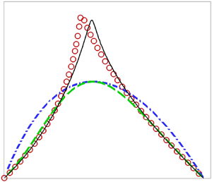
The temporal growth rates  $\sigma _r$, obtained by solving the linear eigenvalue problem, are converted to the spatial growth rate using (2.15). The results are displayed in figure 3 for the subharmonic and fundamental resonances. Comparison is made with the spatial growth rates computed directly by solving the nonlinear eigenvalue problem. Our SIT code for direct spatial solutions has been carefully validated in Xu & Liu (Reference Xu and Liu2022), where good agreement was found between the direct spatial solutions and the predictions by nonlinear parabolized stability equations and direct numerical simulations. For the secondary instability of subharmonic resonance, good agreement is observed (figure 3a). However, in the case of fundamental resonance there is significant difference, especially for large primary-mode amplitude $A$; for example, for $A>0.5$ the error is in the range of 30 %–40 %, and Herbert's transformation fails (figure 3b). This raises the question as to why there is such a contrast of performance. The desire to answer the question prompted us to revisit Gaster's and Herbert's transformations.

Figure 3. Secondary instability growth rates (with  $\beta =2.1$) of a primary Mack mode of different amplitude: comparison of the converted growth rate $\sigma _r/c_r$ (using Herbert's transformation) with that obtained by direct spatial SIT. (a) Subharmonic mode; (b) fundamental mode.
2.2.3. Consistent transformations for secondary instability
For modes in the form of (2.12) with (2.13), the secondary instability defines the dispersion relation:
 \begin{equation} \sigma-\gamma c_{r}=\tilde{\sigma}(\gamma). \end{equation}
Given that the temporal–spatial conversion is established by considering a general dispersion relation, in the complex parameter planes, the specific physical form of the instability, e.g. primary instability of a streamwise homogeneous flow or secondary instability of a spatially periodic flow, does not actually matter because of the analyticity of the dispersion relation. It follows that the required transformations pertinent to the modal form (2.12) may follow directly from (2.3) and (2.9) by replacing  $\omega$ and $\alpha$ by $\mathrm {i}\tilde {\sigma }$ and $-\mathrm {i}\gamma$, respectively. Equivalently, they can be derived by Taylor expansion of (2.16):
 \begin{equation}
\tilde\sigma(S)=\tilde\sigma(T)+\left.\frac{\mathrm{d}
\tilde\sigma}{\mathrm{d} \gamma}
\right|_T [\gamma(S)-\gamma(T)]
+\left.\frac{1}{2}\frac{\mathrm{d}^2
\tilde\sigma}{\mathrm{d}\gamma^2}\right|_T
[\gamma(S)-\gamma(T)]^2+\cdots.
\end{equation}
\begin{equation}
\tilde\sigma(S)=\tilde\sigma(T)+\left.\frac{\mathrm{d}
\tilde\sigma}{\mathrm{d} \gamma}
\right|_T [\gamma(S)-\gamma(T)]
+\left.\frac{1}{2}\frac{\mathrm{d}^2
\tilde\sigma}{\mathrm{d}\gamma^2}\right|_T
[\gamma(S)-\gamma(T)]^2+\cdots.
\end{equation}
Again, there are two ways to relate a temporal mode to its spatial counterpart. Here, we take the more natural and convenient option that the two modes have the same real frequency,  $\tilde {\sigma }_{i}(S)=\tilde {\sigma }_{i}(T)$. With detuning being accounted for by $\epsilon$, we set $\gamma (T)=0$ for a temporal mode, while for a spatial mode $\tilde \sigma _r(S)=0$. Then (2.17) becomes
 \begin{equation} 0=\tilde\sigma_r(T)+\left.\frac{\mathrm{d} \tilde\sigma}{\mathrm{d} \gamma}\right|_T\gamma(S) +\left.\frac{1}{2}\frac{\mathrm{d}^2 \tilde\sigma}{\mathrm{d} \gamma^2}\right|_T\gamma(S)^2+\cdots. \end{equation}
If first-order approximation in (2.18) is made, we have
 \begin{equation} \gamma(S)={-} \tilde\sigma_r(T)\left/\frac{\mathrm{d} \tilde\sigma}{\mathrm{d} \gamma} \right.={-}\sigma_r(T)\left/\frac{\mathrm{d} \tilde\sigma}{\mathrm{d} \gamma}\right. . \end{equation}
The derivative may be computed by taking a purely imaginary increment  $\Delta \gamma =\mathrm {i}\Delta \gamma _i$ from $\gamma =0$ because $\Delta \gamma _i$ can be introduced and corresponding $\sigma$ calculated more easily in our code than with real $\gamma$. It is then convenient to set $\gamma =\mathrm {i}\gamma _i$, and the first-order derivative of $\tilde \sigma$ with respect to $\gamma$ can be expressed as
 \begin{equation} \frac{\mathrm{d}\tilde\sigma}{\mathrm{d}\gamma} =\frac{\mathrm{d}\tilde\sigma_i}{\mathrm{d}\gamma_i} -\mathrm{i}\frac{\mathrm{d}\tilde \sigma_r}{\mathrm{d}\gamma_i} =\left(\frac{\mathrm{d}\sigma_i}{\mathrm{d}\gamma_i}-c_r\right) -\mathrm{i}\frac{\mathrm{d}\sigma_r}{\mathrm{d}\gamma_i}, \end{equation}
and evaluated using a finite-difference approximation. Use of (2.19) gives
 \begin{equation} \left. \begin{aligned} \gamma_r(S) & = \displaystyle -\tilde\sigma_r(T)\frac{\mathrm{d}\tilde\sigma_i}{\mathrm{d}\gamma_i} \left/\left[\left(\frac{\mathrm{d}\tilde\sigma_i}{\mathrm{d}\gamma_i}\right)^2 +\left(\frac{\mathrm{d}\tilde\sigma_r}{\mathrm{d}\gamma_i}\right)^2\right]\right.,\\ \gamma_i(S) & = \displaystyle -\tilde\sigma_r(T)\frac{\mathrm{d}\tilde\sigma_r}{\mathrm{d}\gamma_i} \left/\left[\left(\frac{\mathrm{d}\tilde\sigma_i}{\mathrm{d}\gamma_i}\right)^2 +\left(\frac{\mathrm{d}\tilde\sigma_r}{\mathrm{d}\gamma_i}\right)^2\right]\right. \end{aligned} \right\} \end{equation}
or
 \begin{equation} \gamma_r(S)={-}\dfrac{\sigma_r(T)\left(\dfrac{\mathrm{d}\sigma_i}{\mathrm{d}\gamma_i}-c_r\right)} {\left(\dfrac{\mathrm{d}\sigma_i}{\mathrm{d}\gamma_i}-c_r\right)^2 +\left(\dfrac{\mathrm{d}\sigma_r}{\mathrm{d}\gamma_i}\right)^2},\quad \gamma_i(S)={-}\dfrac{\sigma_r(T)\dfrac{\mathrm{d}\sigma_r}{\mathrm{d}\gamma_i}} {\left(\dfrac{\mathrm{d}\sigma_i}{\mathrm{d}\gamma_i}-c_r\right)^2 +\left(\dfrac{\mathrm{d}\sigma_r}{\mathrm{d}\gamma_i}\right)^2}. \end{equation}
This is the consistent first-order transformation that converts temporal growth rates to spatial growth rates for the secondary instability.
Similar to the case of primary instability, the validity of the transformation (2.19) can be established from the viewpoint of analyticity. The Taylor expansion (2.17) is justified provided that  $|\gamma (S)-\gamma (T)|=|\gamma (S)|$ is small enough (i.e. $\gamma (S)$ is in a vicinity of $\gamma =0$ where $\tilde \sigma (\gamma )$ is analytic), which is guaranteed if the temporal growth rate $\sigma _r$ is small. This is the condition for the transformation (2.19) or (2.22a,b) to be valid. Note that there is no need to impose the extra condition $|\sigma _r|\ll |\sigma _i|$, or $|\gamma _r|\ll |\gamma _i|$, which does not hold for the secondary instability as will be seen later. It now transpires that the first-order transformation (2.22a,b) reduces to Herbert's transformation (2.15) if it turns out that $|\mathrm {d}\sigma /\mathrm {d}\gamma _i| \ll c_r$. In passing, we note that if $|\mathrm {d}\sigma _r/\mathrm {d}\gamma _i|\ll |\mathrm {d}\sigma _i/\mathrm {d}\gamma _i|$, then neglect of $\mathrm {d}\sigma _r/\mathrm {d}\gamma _i$ in (2.22a,b) would lead to a transformation equivalent to Gaster's transformation for the secondary instability (cf. Koch et al. Reference Koch, Bertolotti, Stolte and Hein2000). However, $|\mathrm {d}\sigma _r/\mathrm {d}\gamma _i|\ll |\mathrm {d}\sigma _i/\mathrm {d}\gamma _i|$ is seldom the case for the secondary instability of primary waves. It is likely that for secondary instability, $\sigma _r=O(\sigma _i)$ and $\mathrm {d}\sigma _r/\mathrm {d}\gamma =O(\mathrm {d}\sigma _i/\mathrm {d}\gamma )$. Note that mathematically $\mathrm {d} \tilde \sigma /\mathrm {d} \gamma$ plays a role similar to that of $\mathrm {d} \tilde \omega /\mathrm {d} \alpha$ in the case of the primary instability. The transformation (2.22a,b) is invertible when $\mathrm {d} \tilde \sigma /\mathrm {d} \gamma \neq 0$ and is valid provided that the disc $|\gamma -\gamma (T)|\leq |\gamma (S)-\gamma (T)|$ is free of any singularity and the point where $\mathrm {d} \tilde \sigma /\mathrm {d} \gamma =0$. Interestingly, $\mathrm {d} \tilde \sigma /\mathrm {d} \gamma =0$ occurs when the secondary instability becomes absolute because the former turns out to be the necessary condition for the latter according to the criterion for absolute instability of a general spatially periodic flow (Brevdo & Bridges Reference Brevdo and Bridges1996). As with primary instability, the spatial growth rate is no longer relevant in this case. This connection between the breakdown of the spatial–temporal transformations and absolute instability, whether primary or secondary, is rather intriguing.
If the second-order term in expansion (2.18) is retained, the quadratic equation of  $\gamma (S)$ can be solved to obtain
 \begin{equation} \gamma(S)=\frac{\mathrm{d}\tilde \sigma}{\mathrm{d}\gamma}\left[{-}1 +\sqrt{1 -\left.2\frac{\mathrm{d}^2\tilde\sigma}{\mathrm{d}\gamma^2}\tilde{\sigma}_r(T)\right/ \left(\frac{\mathrm{d}\tilde\sigma}{\mathrm{d}\gamma}\right)^2}\right] \left/\frac{\mathrm{d}^2\tilde\sigma}{\mathrm{d}\gamma^2}\right., \end{equation}
where the second-order derivative is evaluated by using
 \begin{equation} \frac{\mathrm{d}^2\tilde\sigma}{\mathrm{d}\gamma^2} ={-}\frac{\mathrm{d}^2\tilde\sigma}{\mathrm{d}\gamma_i^2} ={-}\frac{\mathrm{d}^2 \sigma}{\mathrm{d}\gamma_i^2} \end{equation}
numerically: we first calculate  $\sigma$ (or $\tilde \sigma$) for $\pm \gamma _i$ (with $\gamma _i\ll 1$) in addition to $\gamma _i=0$ and then a finite difference is applied to obtain the second-order derivative. The temporal–spatial transformation is performed following the flowchart shown in the Appendix. Note again that the calculations involve solving the linear eigenvalue problem, which amounts to little extra cost. Care must be taken when comparing the converted and directly calculated $\gamma$. Note that they are of the forms $\exp ([\gamma x +\mathrm {i} \sigma _i(T) t])$ and $\exp ([\gamma x +(\sigma -\gamma c_r) t])$, respectively. The two are identical if we take $\sigma =\gamma c_r +\mathrm {i}\sigma _i(T)$, i.e. $\tilde \sigma _i=\sigma _i(T)$ in the direct calculation. Conversion will be performed for the most unstable temporal secondary mode. This is of course inadequate for solving the signalling problem, i.e. for tracing the spatial development of a general time-periodic disturbance with a fixed frequency, $\tilde \omega$ say, because that would require calculation and superposition of all secondary unstable modes with a fixed $\tilde \omega$. However, it is possible to trace the downstream evolution of an unstable secondary mode with a fixed frequency $\tilde \omega$, in which case $\epsilon$ is chosen such that $(1+\epsilon )\alpha c_r-\sigma _i(T;\epsilon )=\tilde \omega$ according to (2.12).
3. Applications and validations of the transformations
3.1. Primary instability of a mixing layer
Since the high accuracy of Gaster's transformation for viscous shear instability has been well established, we consider inviscid Rayleigh instability, using a mixing layer with a non-dimensional base-flow profile,
 \begin{equation} U(y)=\left[(1+\chi)+(1-\chi)\mathrm{tanh}(y)\right]/2 , \end{equation}
as a vehicle, where  $\chi$ stands for the ratio of the velocities of the two merging free streams. The spatial instability has been well studied (Michalke Reference Michalke1965), and absolute instability arises when $\chi <\chi _c=-0.136$ (Huerre & Monkewitz Reference Huerre and Monkewitz1985), but existing transformations did not perform well due in part to the relatively large growth rate (Peng & Williams Reference Peng and Williams1987; Roychowdhury & Sreedhar Reference Roychowdhury and Sreedhar1992). For the case of $\chi =0$, we re-calculated the spatial eigenvalues $\alpha$ in the entire instability band, as well as the temporal eigenvalues $\omega$. In order to resolve neutral and nearly neutral modes, we employed a viscous eigenvalue solver, in which a very high Reynolds number, $10^8$, is specified. The temporal eigenvalues were then converted to their spatial counterparts using different transformations. The comparison is shown in figure 4. In order to shed light on the validity and accuracy of the transformations, the first- and second-order derivatives, $\mathrm {d}\omega /\mathrm {d}\alpha$ and $\mathrm {d}^2\omega /\mathrm {d}\alpha ^2$, are computed and displayed in figure 5. The first-order transformation (2.3), which involves the complex group velocity, gives accurate wavenumber $\alpha _r$ in the entire instability band (figure 4a), and more significantly accurate spatial growth rates as well, except for nearly most unstable modes. The error there can be as large as $20\,\%$ due to large growth rates, and may be reduced by applying the second-order transformation (2.9). Indeed, the latter turned out to give both the spatial growth rates and the wavenumbers almost indistinguishable to graphical precision from the results of direct spatial stability analysis. In contrast, the original Gaster's transformation does not give spatial growth rate or wavenumber $\alpha _r$ with satisfactory accuracy. Note that at $\omega _r\approx 0.22$, where the growth rate $\omega _i$ attains its maximum, the results given by the first-order and Gaster's transformations overlap, due to the fact that $\mathrm {d}\omega _i/\mathrm {d}\alpha =0$ (figure 5) so that the first-order transformation reduces to Gaster's transformation. Appreciable error exists for nearly neutral modes $\omega _r\approx 0.5$ despite the fact that not only is $-\alpha _i$ (or $\omega _i$) small, but also $|\alpha _i|\ll |\alpha _r|$ (or $|\omega _i|\ll |\omega _r|$). This indicates that the above condition is not sufficient for the validity of Gaster's transformation, contrary to the suggestion of $|\alpha _i/\alpha _r|\ll 1$, which was made, for example, in Peng & Williams (Reference Peng and Williams1987), and has probably been accepted by many researchers.

Figure 4. Spatial eigenvalues for inviscid instability of a mixing layer (3.1) with  $\chi =0$: comparison between the directly calculated spatial mode (symbols) and the converted results using Gaster's transformation (dash-dotted line), first-order transformation (2.6a,b) (dashed line) and second-order transformation (2.9) (solid line). (a) Wavenumber $\alpha _r$ versus $\omega _r$; (b) spatial growth rate $-\alpha _i$ versus $\omega _r$.

Figure 5. The real parts, imaginary parts and modulus of (a)  $\mathrm {d} \omega /\mathrm {d} \alpha$ and (b) $\mathrm {d}^2 \omega /\mathrm {d} \alpha ^2$ versus the frequency $\omega _r$ for the mixing layer (3.1) with $\chi =0$. The analytically given group velocities of the long-wavelength mode and nearly neutral mode are marked by symbols (square and circles).
Considerable discrepancy between the converted growth rates using Gaster's transformation and directly calculated ones exists also in the low-frequency limit  $\omega _r\ll 1$, where $\alpha _r\ll 1$ and the growth rates are small ( $|\omega _i|$, $|\alpha _i|\ll 1$), showing that the past assertion that Gaster's transformation ‘is valid only very close to the neutral point corresponding to $\alpha _r=0$ and $\alpha _i=0$’ (Roychowdhury & Sreedhar Reference Roychowdhury and Sreedhar1992) is completely erroneous. Clearly, that $|\omega _i|$ or $|\alpha _i|$ is small does not guarantee the validity of Gaster's transformation. What is required instead is (2.7), which is unfortunately not warranted since $\mathrm {d}\omega _i/\mathrm {d}\alpha =O( \mathrm {d}\omega _r/\mathrm {d}\alpha )=O(1)$ in the majority of the instability band as figure 5 shows. Specifically, in the long-wavelength limit ( $\alpha \ll 1$), the dispersion relation reduces asymptotically to (Drazin & Howard Reference Drazin and Howard1962)
 \begin{equation} \omega=\tfrac{1}{2}\left[ (1+\chi)+\mathrm{i}(1-\chi)\right]\alpha, \end{equation}
and so the group velocity  $c_g=[ (1+\chi )+\mathrm {i}(1-\chi ) ]/2$ is complex; for $\chi =0$, $c_g=(1+\mathrm {i})/2$, whose real and imaginary parts are the same. On the other hand, for nearly neutral modes, the group velocity is found as (Wu & Tian Reference Wu and Tian2012)
 \begin{equation} c_g=\tfrac{1}{2}(1-\chi)[1-\mathrm{i}(2/{\rm \pi})(1-\chi)/(1+\chi)], \end{equation}
which is again complex, and specifically  $c_g=(1-2\mathrm {i}/{\rm \pi} )/2$ for $\chi =0$. The numerical values of $c_g$ at these two limits are in good agreement with the analytical ones (figure 5a). The behaviours of $\mathrm {d}\omega _i/\mathrm {d}\alpha$ near the peak growth and neutrality show that $|\omega _i|\ll |\omega _r|$ is neither necessary nor sufficient condition for (2.7). In contrast to Gaster's transformation, the first-order transformation (2.3) is not subject to this restriction, and it provides accurate spatial growth rates.
Figure 6 shows the converted and directly calculated spatial eigenvalues for  $\chi =-0.13$, which is just above the critical value for the onset of absolute instability ( $\chi <\chi _c=-0.136$) (Huerre & Monkewitz Reference Huerre and Monkewitz1985); the latter was implied by an almost vertical slope of the $\alpha _r$– $\omega _r$ curve (figure 6a). The prediction by Gaster's transformation is rather unsatisfactory. The first-order transformation (2.3) is accurate except for $\omega _r$ in the interval $(0.12, 0.26)$ centred at the maximum growth rate, where appreciable error up to $40\,\%$ arises. The second-order transformation (2.9) performs satisfactorily in the entire instability band, with only minor discrepancy near the peak growth. This difference is caused by the truncation of the Taylor expansion, and may further be reduced by using a higher-order transformation. However, there is little point in pursuing this since the error is already very small. It is worth emphasizing that the accuracy is realized despite the fact that $-\alpha _i$ is comparable with $\alpha _r$. It is also worth pointing out that the abrupt and seemingly non-smooth change of $-\alpha _i$ with $\omega _r$ in spatial instability (figure 6b) prompted us to check if a similar behaviour occurs with $\omega$ versus $\alpha$ for temporal modes since this may affect accurate evaluation of ${\mathrm {d}}\omega /{\mathrm {d}}\alpha$ and ${\mathrm {d}}^2\omega /{\mathrm {d}}\alpha ^2$ using finite differences. Interestingly, both $\omega _r$ and $\omega _i$ turn out to vary rather gradually with $\alpha$.

Figure 6. Spatial eigenvalues for inviscid instability of the mixing layer (3.1) with  $\chi =-0.13$: comparison between the directly calculated spatial mode (symbols) and the converted results using Gaster's transformation (dash-dotted line), first-order transformation (dashed line) and second-order transformation (solid line). (a) Wavenumber $\alpha _r$ versus $\omega _r$; (b) spatial growth rate $-\alpha _i$ versus $\omega _r$.
3.2. Primary instability of a jet
The transformations are also applied to a plane jet, which supports two types of modes, sinuous and varicose modes. The Bickley jet profile,
 \begin{equation} U(y)={\mathrm{sech}}^2 y,\end{equation}
is taken as a convenient example, and the transformed spatial eigenvalues using the three transformations are displayed in figure 7 and compared with those of direct calculations. For the varicose mode, all three transformations give practically the same result for the whole instability band, but a zoomed view reveals that the second-order transformation is more accurate. For the sinuous mode, the predictions by all three transformations are highly accurate for  $\omega _r>0.5$, but for $\omega _r<0.5$ the transformed growth rates using Gaster's and first-order transformations deviate considerably from the directly calculated values (figure 7b). The error in the wavenumbers is rather minor, just discernable with Gaster's transformation. The converted spatial growth rates by the second-order transformation (2.9) overlap those of the direct calculation in the entire band of the sinuous instability. It is worth noting that while grossly inaccurate for nearly neutral modes on the mixing layer, Gaster's transformation turns out to be accurate for nearly neutral (sinuous and varicose) modes on the jet. This can be attributed to the fact that the group velocities $c_g=1.0051-0.2224\mathrm {i}$ and $0.6039-0.1670\mathrm {i}$ for the sinuous and varicose modes, respectively (Drazin & Howard Reference Drazin and Howard1962), and so with the ratio $|c_{g,i}/c_{g,r}|$ being approximately $1/4$, the relative error due to neglecting $c_{g,i}$ is merely $7\,\%$.

Figure 7. Spatial eigenvalues for inviscid instability of a jet with profile (3.4): comparison between the directly calculated spatial modes (symbols) and the converted results using Gaster's transformation (dash-dotted line), first-order transformation (dashed line) and second-order transformation (solid line). (a) Wavenumber  $\alpha _r$ versus $\omega _r$; (b) spatial growth rate $-\alpha _i$ versus $\omega _r$.
The plane jet is interesting because the dispersion relations in the long-wavelength limit are non-analytic, which has implications for the validity of the transformations (Brevdo Reference Brevdo1992). For the varicose mode, as  $\alpha \rightarrow 0$ the dispersion relation has the asymptotic approximation (Drazin & Howard Reference Drazin and Howard1962)
 \begin{equation} \omega=a_0\alpha + a_1 \mathrm{e}^{2{\rm \pi} \mathrm{i}/3}\alpha^{5/3}, \end{equation}
where  $a_0$ and $a_1$ are real constants; for the profile (3.4), $a_0=1$ and $a_1=({\rm \pi} /4)^{2/3}$. Clearly, with $\alpha =0$ being a branch point, the function (3.5) is non-analytic at $\alpha =0$. It follows that the group velocity $c_g=a_0 + \tfrac {5}{3} a_1 \mathrm {e}^{2{\rm \pi} \mathrm {i}/3}\alpha ^{2/3}\approx a_0$ to leading-order accuracy. Thus the first-order transformation reads
 \begin{equation} \alpha(S)-\alpha(T)={-}{\mathrm{i}}\frac{\sqrt{3}}{2}a_1 [\alpha(T)]^{5/3} \left/\left[a_0 + \frac{5}{3} a_1 \mathrm{e}^{2{\rm \pi}\mathrm{i}/3}[\alpha(T)]^{2/3}\right]\right., \end{equation}
and the converted spatial growth rate
 \begin{equation} -\alpha_i=\frac{\sqrt{3}}{2} a_1 a_0^{{-}8/3}\omega^{5/3}. \end{equation}
On the other hand, the dispersion relation (3.5) can be inverted to give
 \begin{equation} \alpha=\omega/a_0 -a_1 a_0^{{-}8/3}\mathrm{e}^{2{\rm \pi}\mathrm{i}/3}\omega^{5/3},\end{equation}
the imaginary part of which gives the same spatial growth rate  $-\alpha _i$ as (3.7). Since the group velocity $c_g$ and the phase velocity $c$ are both approximately $a_0$, which is real, Gaster's transformation stands as a valid approximation, as the numerical results in figure 7 confirm. For the weak non-analyticity of (3.5), the branch point $\alpha =0$ remains outside of the disc on the $\alpha$ plane (see figure 1), $|\alpha -\alpha (T)|\leq |\alpha (S)-\alpha (T)|=O(\omega ^{5/3})$, since $\alpha (T) =O(\omega )$ so that the Taylor series is deemed convergent. Note further that $\mathrm {d}^2\omega /\mathrm {d}\alpha ^2=O(\alpha ^{-1/3})$, but $({\mathrm {d}^2\omega }/{\mathrm {d}\alpha ^2})[\alpha (S)-\alpha (T)]^2=O(\alpha ^3)$, much smaller than the first-order term $({\mathrm {d}\omega }/{\mathrm {d}\alpha })[\alpha (S)-\alpha (T)]$, which is of $O(\alpha ^{5/3})$, and higher-order terms are progressively smaller in the limit $\alpha \rightarrow 0$, indicating that the Taylor series is asymptotic as well. Hence the present weak non-analyticity does not affect the validity of the transformations even in the vicinity of the branch point singularity.
For the sinuous mode, as  $\alpha \rightarrow 0$ the dispersion relation reads (Drazin & Howard Reference Drazin and Howard1962)
 \begin{equation} \omega=\mathrm{i} a_0\alpha^{3/2}+a_1\alpha^2+O(\alpha^{5/2}),\end{equation}
where  $a_0$ and $a_1$ are real constants; for the profile (3.4) $a_0=\sqrt {2/3}$ and $a_1=1$, and (3.9) turns out to hold up to $\omega _r=0.05$ (figure 8a). The group velocity $c_g=2 a_1 \alpha +\mathrm {i} \frac {3}{2} a_0\alpha ^{1/2}$, clearly showing that $c_{g,i}\gg c_{g,r}$, and so Gaster's transformation is not expected to hold. Indeed, application of this transformation gives
 \begin{equation} \alpha(S)-\alpha(T)={-}{\mathrm{i}} \frac{a_0}{2a_1}[\alpha(T)]^{1/2}+O\left(\alpha(T)\right), \end{equation}
indicating that the branch point  $\alpha =0$ is within the disc $|\alpha -\alpha (T)|<({a_0}/{2a_1})[\alpha (T)]^{1/2}$. Gaster's transformation is therefore invalid, and this explains its very poor performance displayed in figure 8(b). In contrast, the consistent first-order transformation gives
 \begin{equation} \alpha(S)-\alpha(T)={-}{\mathrm{i}} a_0[\alpha(T)]^{3/2}\left/[3{\mathrm{i}} a_0 [\alpha(T)]^{1/2}/2+2 a_1\alpha(T)]\right., \end{equation}
and so the spatial growth rate is found as
 \begin{equation}
-\alpha_i=2a_0a_1(\omega/a_1)^{3/4} \left/[
4a_1^2(\omega/a_1)^{1/2}+9a_0^2/4]\right. \approx
\frac{8}{9}a_0^{{-}1}a_1(\omega/a_1)^{3/4},
\end{equation}
\begin{equation}
-\alpha_i=2a_0a_1(\omega/a_1)^{3/4} \left/[
4a_1^2(\omega/a_1)^{1/2}+9a_0^2/4]\right. \approx
\frac{8}{9}a_0^{{-}1}a_1(\omega/a_1)^{3/4},
\end{equation}
where use has been made of the fact that  $\omega _r=a_1[\alpha (T)]^2$ for a temporal mode. The direct inversion of (3.9) gives
 \begin{equation} \alpha= a_0^{{-}2/3}\mathrm{e}^{-\mathrm{i}{\rm \pi}/3}\omega^{2/3} + \frac{2}{3}a_1a_0^{{-}2}\omega+O(\omega^{4/3}), \end{equation}
which gives the spatial growth rate
 \begin{equation} -\alpha_i=\frac{\sqrt{3}}{2}a_0^{{-}2/3}\omega^{2/3}. \end{equation}
Curiously, this is different from (3.12), and there arises the question concerning the relation between the two. To answer the question, we note that for the dispersion relation (3.9),  $\mathrm {d}\omega /\mathrm {d}\alpha =O(\alpha ^{1/2})$ and $\mathrm {d}^2\omega /\mathrm {d}\alpha ^2=O(\alpha ^{-1/2})$, and so the first-order term $({\mathrm {d}\omega }/{\mathrm {d}\alpha })[\alpha (S)-\alpha (T)]=O(\alpha ^{3/2})$, the second-order term $({\mathrm {d}^2\omega }/{\mathrm {d}\alpha ^2})[\alpha (S)-\alpha (T)]^2=O(\alpha ^{3/2})$ and higher-order terms remain of this order in the limit $\alpha \rightarrow 0$. Hence, unlike the varicose mode (3.5), the non-analyticity of the sinuous mode (3.9) renders the Taylor series non-asymptotic. This explains why (3.12) differs from the asymptotic approximation (3.14).

Figure 8. Temporal and spatial eigenvalues for inviscid instability of a jet with profile (3.4): comparison between the directly calculated spatial modes (symbols) and the converted results using Gaster's transformation (dash-dotted line), first-order transformation (dashed line) and second-order transformation (solid line). (a) Temporal eigenvalues versus wavenumber  $\alpha$; (b) spatial growth rates versus frequency $\omega _r$.
On the other hand, it follows from (3.11) that
 \begin{equation} |\alpha(S)-\alpha(T)|<\frac{2}{3}\alpha(T),\end{equation}
indicating that the branch point  $\alpha =0$ is outside of the disc $|\alpha -\alpha (T)|<\tfrac {2}{3}\alpha (T)$, and the Taylor series must therefore be convergent. Alternatively, by close inspection it may be deduced that for $n\geq 3$, the $n$th term in the expansion has the expression
 \begin{equation} \frac{\mathrm{d}^n\omega}{\mathrm{d}\alpha^n} \left[\alpha(S)-\alpha(T)\right]^n =({-}1)^n\frac{{\mathrm{i}} 3a_0(2n-5)!!}{2^n n!} [\alpha(T)]^{{3}/{2}-n} \left[\alpha(S)-\alpha(T)\right]^n. \end{equation}
The ratio test shows that the radius of convergence is  $\alpha (T)$, which is the distance of $\alpha (T)$ to the branch point as expected by the consideration of analyticity. From this and (3.15) follows the convergence of the Taylor expansion. Both arguments lead to the conclusion that (3.12) and its second-order version represent the truncations of a convergent series. The branch-point singularity of the sinuous mode (3.9) does not, even in its vicinity, cause breakdown of transformations (2.3) or (2.9). Figure 8(b) shows that the analytical approximation (3.12) follows closely its numerical equivalent first-order transformation (2.3), while the analytical inversion (3.14) is in good agreement with the direct numerical spatial solution. Remarkably, the second-order transformation (2.9) proves to be accurate for all $\omega _r>0$.
3.3. Secondary instability of Görtler vortices
Temporal-to-spatial transformation is even more relevant when secondary instability of Görtler vortices or streaks is studied because for a bi-global eigenvalue problem computation of the spatial growth rates is much more difficult and costly than solving a temporal instability problem. As an illustration, we consider secondary instability of Görtler vortices which were calculated by Xu et al. (Reference Xu, Zhang and Wu2017) pertaining to the measurement at  $x^*=100$ cm in the experiment of Swearingen & Blackwelder (Reference Swearingen and Blackwelder1987). The bi-global eigensolutions are obtained by solving an inviscid instability problem and so only unstable modes are found. Figure 9 displays the directly calculated spatial eigenvalues and the converted ones using Gaster's transformation (1.3) as well as the first- and second-order transformations, (2.3) and (2.9). Gaster's and the first-order transformations both give growth rates and wavenumbers with satisfactory accuracy. Their comparable performance can be attributed to the fact that $\mathrm {d}\omega _i/\mathrm {d}\alpha$ is approximately $1/4$ of $\mathrm {d}\omega _r/\mathrm {d}\alpha$ (figure 10a) so that the condition (2.7) may be considered as being satisfied approximately, which means that the difference between the results is only approximately $7\,\%$. The good accuracy of these transformations is also due to the fact that $\mathrm {d}^2 \omega /\mathrm {d}\alpha ^2$ is rather small as figure 10(b) indicates. Figure 10(b) shows that minor differences from the direct spatial solution arise near the peak growth rate, and they are eliminated almost completely when the second-order transformation (2.9) is applied.

Figure 9. Spatial secondary instability characteristics of Görtler vortices: comparison of the directly calculated spatial modes (symbols), Gaster's transformation (dash-dotted line), first-order transformation (2.6a,b) (dashed line) and second-order transformation (2.9) (solid line). (a) Wavenumber  $\alpha _r$ versus $\omega _r$; (b) spatial growth rate $-\alpha _i$ versus $\omega _r$.

Figure 10. The real parts, imaginary parts and modulus of (a)  $\mathrm {d} \omega /\mathrm {d}\alpha$ and (b) $\mathrm {d}^2 \omega /\mathrm {d}\alpha ^2$ versus the frequency $\omega _r$.
3.4. Secondary instability of two-dimensional waves
We first revisit the cases shown in figure 3, which indicate that Herbert's transformation failed for the fundamental resonance. The data for temporal secondary instability are now converted to spatial secondary instability characteristics using the newly developed first- and second-order transformations, (2.22a,b) and (2.23). The results are shown in figure 11. For the subharmonic resonance (figure 11a), the first-order transformation (2.3) and Herbert's transformation (2.15) both give correct results, in good agreement with those given by direct spatial secondary instability analysis. A zoomed view indicates that the first-order transformation is actually more accurate than Herbert's transformation, while the predictions by the second-order transformation and direct spatial calculations are practically identical. However, for the fundamental resonance (figure 11b), the first-order and Herbert's transformations give reasonably accurate spatial growth rates only when the primary-mode amplitude is small,  $A<0.35$ and $A<0.2$, respectively, beyond which the accuracy deteriorates as $A$ increases. When $A>0.5$, Herbert's transformation gives wrong spatial growth rates while the first-order transformation (2.22a,b) is also grossly inaccurate due to fairly large growth rates. Using the second-order transformation (2.23), the converted growth rates turn out to have satisfactory accuracy. The reasons why Herbert's transformation works and is accurate for subharmonic modes but not for fundamental modes are discussed later.

Figure 11. Secondary instability characteristics of a Mack mode with different amplitude  $A$: comparison between spatial eigenvalues directly calculated by spatial SIT (symbols) with the converted results using the first-order transformation (2.22a,b) (dashed line), the second-order transformation (2.23) (solid line) and Herbert's transformation (dash-dotted line). (a) Subharmonic modes; (b) fundamental modes. The secondary instability modes have spanwise wavenumber $\beta =2.1$.
We now turn to applications of the transformations to detuned resonance, and consider first the case with a moderate primary-wave amplitude  $A=0.45$. The converted and directly calculated spatial eigenvalues, $\gamma _r$ and $\gamma _i$, for the full range of detuning parameter $\epsilon \in [0,0.5]$, are shown in figure 12. Herbert's transformation gives accurate growth rate $\gamma _r$ for $\epsilon >$0.16, but deteriorates immediately when $\epsilon < 0.16$. The second-order transformation is able to predict the growth rate with high accuracy for the entire range of $\epsilon$. The first-order transformation performs equally well except for $\epsilon <0.02$. These two transformations also give accurate $\gamma _i$ for $\epsilon >0.04$, below which $\gamma _i$ is slightly under-predicted by the second-order transformation but significantly by the first-order transformation (figure 12b). There is no corresponding formula for $\gamma _i$ in Herbert's transformation. If $\sigma _i/c_r$ is used, the converted $\gamma _i$ is in agreement with the directly calculated result only for $\epsilon >0.3$, but the two bear little resemblance for $\epsilon <0.3$.

Figure 12. Spatial eigenvalues for secondary instability of detuned resonance: comparison of the spatial SIT (symbols), Herbert's transformation (dash-dotted line), first-order transformation (2.22a,b) (dashed line) and second-order transformation (2.23) (solid line) when the primary-wave amplitude  $A=0.45$. (a) Real parts of the eigenvalues; (b) imaginary parts of the eigenvalues. The secondary instability modes have spanwise wavenumber $\beta =2.1$.
In order to distinguish further the performances of different transformations, a case with a large amplitude of  $A=0.88$ is chosen. For such a large value of $A$, there exist multiple unstable secondary modes at each $\epsilon$. We focus on the most unstable one. The converted spatial eigenvalues, $\gamma _r$ and $\gamma _i$, for the full range of detuning parameter $\epsilon \in [0,0.5]$, are plotted in figure 13. The first- and second-order transformations give almost the same and sufficiently accurate results for $\epsilon >0.04$. Herbert's transformation turns out to be just as accurate for $\epsilon >$0.18, but appreciable difference exists for $\epsilon <0.18$. Nevertheless, it still gives reasonably accurate spatial eigenvalues for $\epsilon >0.04$. When $\epsilon$ is below 0.04, Herbert's and the first-order transformations are highly inaccurate, significantly under-predicting the spatial growth rate $\gamma _r$ with the respective errors being the greatest at $\epsilon =0$. The second-order transformation (2.23) is highly accurate, giving spatial eigenvalues in almost perfect agreement with those from direct spatial eigenvalue calculations for $0\leq \epsilon \leq 0.02$. However, a complication arises in the small interval $0.02<\epsilon <0.04$. Temporal stability analysis shows that the two most unstable temporal modes are fairly close to each other. This is likely to undermine the validity of our transformations since the latter are invalid in the extreme (limiting) case where two modes coalesce. The precise impact of near coalescence of two modes on the validity and accuracy of the transformations remains to be fully analysed. We speculate that it reduces the radius of convergence and/or the rate of convergence with respect to the order of the Taylor expansion. On the other hand, while the most unstable temporal mode remains on the same branch as $\epsilon$ varies, the spatial stability analysis shows that there is a crossover of the two most unstable spatial modes at $\epsilon \approx 0.04$. In the interval $0.02<\epsilon <0.04$, the comparison between the directly calculated and transformed eigenvalues becomes complicated, and a satisfactory agreement is denied. The resolution is left for future investigation. It is worth noting that the growth rates $\gamma _r$ are appreciably greater than the wavenumber $\gamma _i$ for $\epsilon >0.05$; nevertheless, the transformations (2.22a,b) and (2.23) performed well, confirming that $|\gamma _r/\gamma _i|\ll 1$ or $|\sigma _r/\sigma _i|\ll 1$ is not a necessary condition for them to be valid. Since the full frequency shift is $\sigma _i-(\gamma _i+\epsilon \alpha )c_r$, i.e. $\tilde \sigma _i-\epsilon \alpha c_r$, we plot $\gamma _r$ versus $\sigma _i-(\gamma _i+\epsilon \alpha )c_r$ as well as $\tilde {\sigma }_i$. The results are displayed in figure 14, demonstrating again the satisfactory performance of the second-order transformation (2.23). It is worth noting that for the subharmonic and fundamental resonances $\tilde \sigma _i =0$, which indicates that the secondary modes and the primary wave have the same phase speed. For $0<\epsilon <0.5$, $|\tilde \sigma _i|<0.01$ ( $|\tilde \sigma _i/(\alpha c_r)|<0.005$) is rather small, which means the most physically relevant secondary modes tend to propagate at almost the same phase speed as that of the primary wave, that is, they are synchronized or ‘phase locked’ (Wu & Stewart Reference Wu and Stewart1996; Wu, Stewart & Cowley Reference Wu, Stewart and Cowley1996).

Figure 13. Spatial eigenvalues for secondary instability of detuned resonance: comparison of the spatial SIT (symbols), Herbert's transformation (dash-dotted line), first-order transformation (2.22a,b) (dashed line) and second-order transformation (2.23) (solid line) when the primary-wave amplitude  $A=0.88$. (a) Real parts of the eigenvalues; (b) imaginary parts of the eigenvalues. The secondary instability modes have spanwise wavenumber $\beta =2.1$.

Figure 14. The growth rate  $\gamma _r$ versus the full frequency shift $\tilde \sigma _i-\epsilon \alpha c_r$ as well as $\tilde \sigma _i$: comparison of the spatial SIT (symbols), first-order transformation (2.22a,b) (dashed line) and second-order transformation (2.23) (solid line) when the primary-wave amplitude $A=0.88$.
In order to understand the performances of the transformations, we calculated  $\mathrm {d}\sigma /\mathrm {d}\gamma$ and $\mathrm {d}^2\sigma /\mathrm {d}\gamma ^2$, and the outcomes are shown in figure 15. For the subharmonic mode $(\epsilon =0.5)$, $\mathrm {d}\sigma _r/\mathrm {d}\gamma$ and $\mathrm {d}\sigma _i/\mathrm {d}\gamma$ are of $O(10^{-2})$, and are thus negligible in comparison with $c_r$, which is $c_r=0.90137$. Consequently, the transformation (2.22a,b) is well approximated by Herbert's transformation. For $0.05<\epsilon <0.5$, $\mathrm {d}\sigma _r/\mathrm {d}\gamma$ and $\mathrm {d}\sigma _i/\mathrm {d}\gamma$ are rather moderate, being less than $0.08$, and so neglecting them does not cause significant error, which is why Herbert's transformation also performed fairly well for detuned modes in this range of $\epsilon$. It should be emphasized that the smallness of $\mathrm {d}\sigma _r/\mathrm {d}\gamma$ and $\mathrm {d}\sigma _i /\mathrm {d}\gamma$ is established a posteriori by numerical computation; there is no a priori reason or analysis for one to conclude that they must be small. In this sense, Herbert's transformation works primarily by coincidence, and is purely empirical in its nature, unlike a proper mathematical approximation in which the error could in principle be made arbitrarily small. Indeed, for $0\leq \epsilon \leq 0.05$, which includes the fundamental resonance ( $\epsilon =0)$, $\mathrm {d}\sigma _r/\mathrm {d}\gamma$ and $\mathrm {d}\sigma _i /\mathrm {d}\gamma$ acquire rather sizeable values greater than $0.2$. The consistent first-order transformation (2.22a,b) needs to be used at least, and this leads to better predictions than does Herbert's transformation. However, due to increased growth rate and the fact that the second-order derivative $\mathrm {d}^2 \sigma /\mathrm {d} \gamma ^2$ acquires large values (figure 15b), the second-order term in the expansion (2.18) becomes appreciable. With this term included, the second-order transformation (2.23) is able to predict spatial secondary instability characteristics with adequate accuracy for $0\leq \epsilon \leq 0.02$.

Figure 15. The real parts, imaginary parts and modulus of (a)  $\mathrm {d} \sigma /\mathrm {d} \gamma$ and (b) $\mathrm {d}^2 \sigma / \mathrm {d} \gamma ^2$ versus the detuning parameter $\epsilon$ when the primary-wave amplitude $A=0.88$.
4. Summary and conclusions
In this paper, we have revisited the transformations of temporal and spatial growth rates of shear instabilities in weakly non-parallel flows. As an effort to clarify the validity and accuracy of the widely used Gaster's and Herbert's transformations for primary and secondary instabilities, respectively, we derived the consistent transformations simply by using Taylor expansion of the dispersion relation for the instability. A point that was emphasized in the present paper but seemed overlooked previously is that the conversions between temporal and spatial growth rates may be established for modes having the same frequency or wavenumber, with the former being more natural. The validity of the transformations derived, consisting of first- and second-order versions, is guaranteed by analyticity of the dispersion relation, while the accuracy requires the growth rates to be small. The condition that the temporal/spatial growth rates are much smaller than frequencies/wavenumbers is not required, and further light on this issue was shed by the discussion of the validity for the neutral modes and in the long-wavelength limit.
For primary instability, the consistent first-order transformation is less restrictive than the original Gaster's transformation, and reduces to the latter under the additional condition that the imaginary part of the complex group velocity is much smaller than its real part, which forms the validity condition of Gaster's transformation together with the requirement of small growth rates. The previously suggested, and perhaps widely accepted, restriction that the temporal/spatial growth rates are much smaller than frequencies/wavenumbers is neither sufficient nor necessary. Since our first-order transformation can be implemented as easily as Gaster's transformation, there is no need to impose the additional condition, which is not readily met.
For secondary instability of a two-dimensional primary mode, our first-order transformation represents a consistent approximation when the growth rates are small, and reduces to Herbert's transformation when  $\mathrm {d}\sigma /\mathrm {d}\gamma$ turns out to be small by coincidence. This additional constraint is satisfied in the case of subharmonic resonance, but not for the fundamental resonance, which explains why Herbert's transformation worked for the former but failed for the latter. Again, since the first-order transformation can be implemented with little extra computation there is no need to impose this extra condition, which is not always warranted.
The transformations derived in the present paper can be implemented within temporal instability analysis to obtain the spatial instability characteristics without substantial extra computational cost. Applications of these transformations to inviscid instability of a mixing layer and a jet, secondary instability of Görtler vortices and secondary instability of primary Mack modes in a supersonic boundary layer indicate that the first-order transformation consistently outperforms Gaster's and Herbert's transformations, and significantly the second-order transformation is able to provide spatial instability characteristics practically identical to those obtained by solving the nonlinear eigenvalue problem for spatial instability. Only in the case where the mode is a double root or two modes come close to each other are the validity and accuracy no longer warranted. This happens only for a very small subset of parameters. The second-order transformation thus stands as a useful tool, and can be employed in the  $\mathrm {e}^{\mathrm {N}}$ method to calculate the N-factor more effectively, saving the need of spatial instability analysis. Furthermore, the transformations can, with appropriate modifications, be applied to other instability problems such as primary cross-flow instability in three-dimensional boundary layers, and the secondary instability of stationary and travelling-wave vortices.
Acknowledgement
The authors are grateful to Professor J. Bai from Northwestern Polytechnical University for his help.
Funding
This work was supported by the NSFC (grant nos 91952202, 92052301, 12172252, 12102361) and the Fundamental Research Funds for the Central Universities (grant no. G2021KY05101).
Declaration of interests
The authors report no conflict of interest.
Appendix
Flowcharts showing computation procedures of temporal–spatial transformations.


