


1. Introduction
Due to its relevance for a wide variety of applications, wall turbulence has been the subject of many studies over the years. Despite the long-standing research activity in this field, wall-bounded turbulence still presents interesting scientific questions and unsolved physical problems, see Townsend (Reference Townsend1980) for a partial review. As a consequence, technological applications still suffer from this lack of knowledge in terms of limited prediction capabilities of turbulence models and of insufficiently general and reliable active/passive techniques for its control and modification. The reason is the strongly inhomogeneous and anisotropic multiscale features of wall turbulence that challenge the development of a complete theory able to explain and predict the interplay between the elementary phenomena composing it. Most of our knowledge on the multiscale dynamics of turbulence is given by Kolmogorov's seminal works on the inertial subrange of turbulence (Frisch Reference Frisch1995). The related theory is based on the groundbreaking intuition of reducing the complex problem of turbulence to its essential features, by assuming homogeneity and isotropy. In these conditions, the main process governing turbulence is the energy cascade between scales which is described by a single scalar parameter – the average dissipation rate (Alexakis & Biferale Reference Alexakis and Biferale2018). However, wall turbulence has a much richer physics that involves, beside energy cascade, anisotropic turbulence production and inhomogeneous spatial fluxes. Such processes are strongly scale and position dependent and lead to a geometrically complex redistribution of energy where reverse energy cascade processes from small to large scales (Piomelli et al. Reference Piomelli, Cabot, Moin and Lee1991; Domaradzki et al. Reference Domaradzki, Liu, Härtel and Kleiser1994; Härtel et al. Reference Härtel, Kleiser, Unger and Friedrich1994; Dunn & Morrison Reference Dunn and Morrison2005) play a fundamental role as unequivocally shown in Cimarelli, De Angelis & Casciola (Reference Cimarelli, De Angelis and Casciola2013); Cimarelli et al. (Reference Cimarelli, De Angelis, Jiménez and Casciola2016). To deal with these more general conditions, the Kolmogorov theory has been extended by Hill (Reference Hill2002) in the form of a balance equation for the second-order structure function. In the case of fully inhomogeneous and anisotropic flow conditions, the generalized Kolmogorov equation describes a field of fluxes in a multidimensional space composed by the three-dimensional (3-D) space of scales and by the 3-D space of positions. Such a six-dimensional augmented-space of turbulence, while giving a complete description of the turbulent phenomena, actually challenges for a rational approach. For this reason, most of the attempts performed so far dealt with paradigmatic flows characterized by statistical symmetries that drastically reduce the order of the augmented-space of turbulence. This is commonly achieved by considering flows with statistically homogeneous directions thus allowing us to reduce the dimensions of the space of positions.
With the aim of understanding wall turbulence, the need to reduce the complexity of turbulence led so far to the application of the Kolmogorov equation to the symmetries of turbulent channel flows. Indeed, the statistical homogeneity of channel flows in the wall-parallel directions reduces the augmented space of turbulence to four dimensions, the 3-D space of scales plus the wall distance. Several fundamental features of wall turbulence have been unveiled by applying the Kolmogorov equation to channel flows, see e.g. Danaila et al. (Reference Danaila, Anselmet, Zhou and Antonia2001), Marati, Casciola & Piva (Reference Marati, Casciola and Piva2004), Cimarelli et al. (Reference Cimarelli, De Angelis and Casciola2013, Reference Cimarelli, De Angelis, Schlatter, Brethouwer, Talamelli and Casciola2015b, Reference Cimarelli, De Angelis, Jiménez and Casciola2016), Hamba (Reference Hamba2018, Reference Hamba2019), Gatti et al. (Reference Gatti, Chiarini, Cimarelli and Quadrio2020) and Zimmerman et al. (Reference Zimmerman, Antonia, Djenidi, Philip and Klewicki2022). Despite the relevance of the results obtained, when dealing with boundary layers, wall turbulence is characterized also by entrainment phenomena at the turbulent/non-turbulent interface (da Silva et al. Reference da Silva, Hunt, Eames and Westerweel2014) whose physical features cannot be addressed in channel flows. Such phenomena make the study of boundary layers of a more general relevance for industrial and geophysical problems. However, the spatial inhomogeneity in the streamwise direction renders boundary layers more challenging for their study in comparison with streamwise-homogeneous channels especially when dealing with the Kolmogorov equation. Indeed, the augmented space of turbulence in boundary layers is composed of five dimensions being the field of fluxes occurring also in the space of streamwise positions, see Yao, Mollicone & Papadakis (Reference Yao, Mollicone and Papadakis2022) where a boundary layer undergoing bypass transition is analysed. This is one of the main reasons for the lack of works studying the generalized Kolmogorov equation in fully developed turbulent boundary layers. It should be noted that the Fourier transform is not applicable in the streamwise direction due to the inhomogeneity in such direction, thus strongly limiting also the use of the formalism given by the spectral energy budget often used in channel flows as a spectral counterpart of the generalized Kolmogorov equation, see e.g. Mizuno (Reference Mizuno2016), Cho, Hwang & Choi (Reference Cho, Hwang and Choi2018), Lee & Moser (Reference Lee and Moser2019) and Wang, Pan & Wang (Reference Wang, Pan and Wang2021). Finally, let us mention that the streamwise inhomogeneity of boundary layers renders also their numerical solution not easy to achieve, see e.g. Schlatter & Örlü (Reference Schlatter and Örlü2010). Indeed, it requires the use of proper inflow and tripping conditions and of very long domains. As an alternative, inflow conditions based on rescaling and recycling methods of the outflow can be used to circumvent the simulation of transition and limiting the domain length but further complicating the computational approach (Lund, Wu & Squires Reference Lund, Wu and Squires1998).
A method to circumvent all these issues is to consider a temporally evolving boundary layer. As recently shown in Kozul, Chung & Monty (Reference Kozul, Chung and Monty2016), the temporal boundary layer presents statistical features very similar to that of the spatially evolving boundary layer. However, the streamwise homogeneity of the temporal boundary layer makes it a very attractive setting to study the physics of turbulent boundary layers (Watanabe, Zhang & Nagata Reference Watanabe, Zhang and Nagata2018; Kozul et al. Reference Kozul, Hearst, Monty, Ganapathisubramani and Chung2020) especially when dealing with sophisticated statistical tools such as the generalized Kolmogorov equation. Furthermore, its ease of set-up and computational cost savings make the temporal boundary layer a very interesting setting also from a computational point of view, see again Kozul et al. (Reference Kozul, Chung and Monty2016). The aim of the present work is thus to extend the analysis of the spatially evolving cascade mechanisms performed so far in channel flows to the settings of turbulent boundary layers. The generalized Kolmogorov equation will be applied to fully developed boundary layers data in order to shed light on the multiscale mechanisms characterizing the different flow regions. A preliminary analysis of the generalized Kolmogorov equation in the setting of a temporal boundary layer has been already published in Cimarelli et al. (Reference Cimarelli, Boga, Pavan, Costa and Stalio2024). It is found that reverse energy cascade mechanisms play a crucial role for the dynamics of near-wall turbulence in accordance with previous works in turbulent channels (Cimarelli et al. Reference Cimarelli, De Angelis and Casciola2013, Reference Cimarelli, De Angelis, Jiménez and Casciola2016). It is also found that the entrainment phenomena acting at the edge of the boundary layer significantly modify the energy transfer mechanisms of the outer region with respect to channels. In particular, reverse energy cascade mechanisms, although weak, are found to persist up to the interface region in analogy with observations reported for turbulent jets in Cimarelli et al. (Reference Cimarelli, Mollicone, Van Reeuwijk and De Angelis2021). The purpose of the present work is to give a physical explanation of these energy transport phenomena in the outer and interface regions of boundary layers. To this aim, the generalized Kolmogorov equation will be analysed in detail by addressing the scale-by-scale contribution of the different terms composing it. Such a study will be also used to provide reduced forms of the scale-by-scale budget for the different flow regions of relevance for turbulence closures. Relevant length scales for the budget will be identified as long as their scaling with the wall distance allows us to characterize the main physical mechanisms dominating the different ranges of scale of the different flow regions. Finally, the use of data from a turbulent channel at the same friction Reynolds number will allow us to recognize which of the observed energy production, transfer and dissipation phenomena can be considered as a robust feature of wall turbulence in general.
The paper is organized as follows. Section 2 provides some details about the simulations performed and about the flow settings. The formalism of the generalized Kolmogorov equation is reported in § 3. The field of fluxes together with the sourcing and sinking mechanisms are analysed in § 4. The scale-by-scale budget characterizing the different flow regions are studied in § 5. Finally, the paper is closed by some concluding remarks in § 6 and by Appendix A where technical details about the generalized Kolmogorov equation formalism are provided.
2. Direct numerical simulations and flow settings
In the present study we analyse data from direct numerical simulations (DNS) of a turbulent channel flow and a temporal boundary layer at a friction Reynolds number  $Re_\tau = u_\tau \delta / \nu = 1500$ where $u_\tau$ is the friction velocity, $\nu$ is the kinematic viscosity of the fluid and $\delta$, in the case of the channel flow, is the half-height of the channel gap, while, in the case of the temporal boundary layer, is the boundary layer thickness.
The channel flow simulation has been performed using a pseudospectral code based on Fourier expansions in the homogeneous directions and Chebyshev polynomials in the wall-normal direction. Time is advanced using a mixed Runge–Kutta and Crank–Nicolson scheme, while the nonlinear terms are calculated in physical space with aliasing errors removed by the 3/2-rule. Full details of the algorithm can be found in Chevalier et al. (Reference Chevalier, Schlatter, Lundbladh and Henningson2007). The domain size is  $(L_x,L_y,L_z) = (37.7, 10.5, 2) \delta$ in the streamwise ( $x$), spanwise ( $y$) and wall-normal ( $z$) directions, respectively. The number of modes used for the spatial discretization is $(N_x,N_y,N_z) = (6144,3456,577)$ thus leading to a physical space resolution in the spatially homogeneous directions $(\Delta x^+,\Delta y^+) = (9.2,4.5)$, see table 1 for additional details. The superscript $+$ is hereafter used to indicate non-dimensionalization with friction units. These DNS data have already been used for studies of wall turbulence in Cimarelli et al. (Reference Cimarelli, De Angelis, Schlatter, Brethouwer, Talamelli and Casciola2015b) to which the reader is referred for further details on the main flow features and on the numerics.
Table 1. Domain extension, spatial discretization and grid resolution of the channel and boundary layer simulations at  $Re_{\tau } = 1500$. The wall-normal resolution $\Delta z_w^+$ is computed at the wall while $\Delta z_\delta ^+$ is evaluated at the location $z^{+} = Re_{\tau }$.

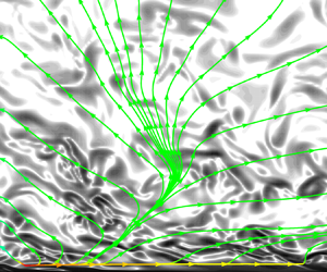
Contrary to the channel flow, the temporal boundary layer is a less investigated flow configuration and for this reason we refer the reader to Kozul et al. (Reference Kozul, Chung and Monty2016) for a detailed description of the numerical set-up and of the main flow features. This type of flow develops in time rather than in space thus allowing us to recover a statistically homogeneous condition both in the streamwise  $(x)$ and spanwise $(y)$ directions, see figure 1(a) for a view of the instantaneous pattern taken by the flow solution. The boundary layer simulation has been performed using the DNS code CaNS (Costa Reference Costa2018) that employs a standard pressure-projection method and a staggered second-order finite-difference scheme for the spatial discretization. Time integration is carried out using a mixed approach. In particular, the viscous terms in the wall-normal direction are integrated implicitly through the use of a Crank–Nicholson scheme, while all the other terms are integrated explicitly by using a three-step Runge–Kutta method with a ${\rm CFL}=0.95$. The domain size in the vertical direction is chosen in order to have a final boundary layer thickness that is $1/3$ the domain height in order to avoid confinement effects, see again Kozul et al. (Reference Kozul, Chung and Monty2016). On the other hand, the lateral sizes of the numerical domain are chosen in order to solve the long and wide structures classically known to occur in wall turbulence. The resulting domain size is $(L_x,L_y,L_z)=(11.9,5.9,2.8)\delta$ and is discretized by using a number of grid points $(N_x,N_y,N_z) = (3072,3072,768)$ that leads to a spatial resolution in the spatially homogeneous directions $(\Delta x^+,\Delta y^+) = (5.8,2.9)$, see table 1 for additional details. In order to improve the statistical convergence of the results, four independent simulations have been carried out by changing the seed of the pseudorandom noise in the initial condition. The present boundary layer data have been already used in Cimarelli et al. (Reference Cimarelli, Boga, Pavan, Costa and Stalio2024) to which we refer the reader for further details about the simulation settings. In the same work, a detailed analysis of the main flow features is also performed in order to provide a physical understanding of the flow and of its main differences with respect to the more classical settings of spatially developing boundary layers.

Figure 1. (a) Instantaneous pattern of enstrophy  $\zeta$ in the boundary layer at $Re_{\tau } = 1500$. The volume rendering reports low and high values of enstrophy from yellow to blue. The two lateral slices show isocontours of enstrophy with values that increase logarithmically from yellow to purple. Finally, the grey isosurface denotes a very small value of enstrophy, $\zeta = 1.4 \times 10^{-6} \langle \zeta \rangle _w$ with $\langle \zeta \rangle _w$ the average value at the wall, in order to show the instantaneous pattern taken by the boundary layer interface in a portion of the domain. (b) Comparison of the mean velocity profiles of the temporal boundary layer and of the channel flow at $Re_\tau = 1500$.
Statistics are computed by performing a spatial average in the streamwise and spanwise directions. In the case of the turbulent channel, a time average is also performed by using different time samples. On the other hand, in the case of the turbulent boundary layer, an ensemble average is also performed between the independent simulations performed. For both flows, the resulting average operator will be denoted as  $\langle {\cdot } \rangle$. The standard Reynolds decomposition will be adopted and denoted as $u_i^* = U_i + u_i$ where $u_i^*$ is the total velocity field and $U_i = \langle u_i^* \rangle$ is the mean velocity field.
The mean velocity profiles of the two flow cases under consideration are reported in figure 1(b). Based on the mean velocity profile and other relevant statistical quantities wall turbulence has been classically divided into physically relevant flow regions depending on the distance from the wall. From an energetic point of view, the peak of activity of turbulence is located in the so-called buffer layer, from where the energy is irradiated towards the wall, in the viscous sublayer, and away from the wall towards the outer region. In this classical view the overlap layer, intermediate between the buffer layer and the outer region, is an equilibrium layer where energy production and dissipation locally balance. In the present work we will stick to this classical decomposition in order to clearly define the relevant regions of the flow that will be analysed through the generalized Kolmogorov equation. In particular, the inner region of the flow will be considered as the region where  $z^+ < 0.2 Re_\tau$ and will be assumed to be composed of a viscous sublayer for $z^+ < 6$, by a buffer layer for $6 < z^+ < 60$ and of an overlap layer for $60 < z^+ < 0.2 Re_\tau$. The rest of the flow will be called the outer region $0.2 Re_\tau < z^+ < Re_\tau$ and, in the case of the boundary layer, will involve also the interface region for $z^+ \approx Re_\tau$.
3. The generalized Kolmogorov equation
The aim of the present work is to investigate the role played by large and small scales in the entrainment processes and in the near-wall self-sustaining mechanisms of turbulence. In order to investigate their multiscale character, the use of two-point statistics is demanding. In this respect, several works in the past have shown that the generalized Kolmogorov equation (Hill Reference Hill2002) represents a sufficiently general statistical formalism to address the multidimensional cascade processes of turbulence from its production to its dissipation. Examples of its application in wall turbulence are Danaila et al. (Reference Danaila, Anselmet, Zhou and Antonia2001), Marati et al. (Reference Marati, Casciola and Piva2004), Cimarelli et al. (Reference Cimarelli, De Angelis and Casciola2013, Reference Cimarelli, De Angelis, Jiménez and Casciola2016), Chiarini et al. (Reference Chiarini, Mauriello, Gatti and Quadrio2022), Yao et al. (Reference Yao, Mollicone and Papadakis2022) and Zimmerman et al. (Reference Zimmerman, Antonia, Djenidi, Philip and Klewicki2022), in thermally driven turbulence are Rincon (Reference Rincon2006); Togni, Cimarelli & De Angelis (Reference Togni, Cimarelli and De Angelis2015), in separated and reattaching flows are Mollicone et al. (Reference Mollicone, Battista, Gualtieri and Casciola2018), Gatti et al. (Reference Gatti, Chiarini, Cimarelli and Quadrio2020) and in turbulent jets and wakes are Burattini, Antonia & Danaila (Reference Burattini, Antonia and Danaila2005), Gomes-Fernandes, Ganapathisubramani & Vassilicos (Reference Gomes-Fernandes, Ganapathisubramani and Vassilicos2015), Portela, Papadakis & Vassilicos (Reference Portela, Papadakis and Vassilicos2017) and Cimarelli et al. (Reference Cimarelli, Mollicone, Van Reeuwijk and De Angelis2021). The generalized Kolmogorov equation is written in terms of the second-order structure function of the fluctuating velocity field
 \begin{equation} \langle \delta q^2 \rangle \equiv \langle \delta u_i \delta u_i \rangle, \end{equation}
where  $\delta u_i \equiv u_i (\boldsymbol {x'},t) - u_i (\boldsymbol {x''},t)$ is the increment of the fluctuating velocity and $\langle {\cdot } \rangle$ denotes ensemble average. Hereafter, we will often refer to the second-order structure function as the scale energy even if such an interpretation is somewhat arguable especially in inhomogeneous flows for large separations, see the discussion in Cimarelli et al. (Reference Cimarelli, De Angelis, Jiménez and Casciola2016) and the possible alternative expression derived in Hamba (Reference Hamba2018). For the theoretical background about the second-order structure function and the generalized Kolmogorov equation, the reader is referred to Appendix A. Here, we develop the formalism for the symmetries of a temporal evolving turbulent boundary layer and turbulent channel. In these settings, the generalized Kolmogorov equation reads
 \begin{align} &\frac{\partial \langle \delta q^2 \rangle}{\partial{t}} + \frac{\partial \langle \delta q^2 \delta u_i \rangle}{\partial{r_i}} + \frac{\partial \langle \delta q^2 \delta U \rangle}{\partial{r_x}} - 2\nu \frac{\partial^2 \langle \delta q^2 \rangle}{\partial{r_i} \partial{r_i}} \nonumber\\ &\qquad + \frac{\partial \langle \delta q^2 \tilde{w} \rangle}{\partial z_c} + \frac{2}{\rho} \frac{\partial \langle \delta p \delta w \rangle}{\partial z_c} - \frac{\nu}{2} \frac{\partial^2 \langle \delta q^2 \rangle}{\partial {z_c}^2}\nonumber\\ &\quad ={-} 2 \langle \delta u \delta w \rangle \widetilde{\left ( \frac{{\rm d}U}{{\rm d}z} \right )} - 2 \langle \delta u\, \tilde{w} \rangle\, \delta\!\left(\frac{{\rm d}U}{{\rm d}z} \right ) - 4\langle \tilde{\epsilon} \rangle, \end{align}
where  $U=U(z,t)$ is the mean streamwise velocity, $\boldsymbol {r} = \boldsymbol {x'}- \boldsymbol {x''}$ is the two-point separation vector, $\boldsymbol {x_c} = (\boldsymbol {x'}+ \boldsymbol {x''})/2$ is the position vector of the midpoint and $\tilde {\cdot }$ denotes the two-point average. Finally,
 \begin{equation} \epsilon = \nu \frac{\partial u_i}{\partial x_j} \frac{\partial u_i}{\partial x_j} \end{equation}
is the turbulent pseudodissipation. Here,  $x$,
$x$,  $y$ and $z$ (
$z$ ( $u$,
$u$,  $v$ and $w$) denote the streamwise, spanwise and wall-normal directions (velocities). For the sake of clarity, the generalized Kolmogorov equation (3.2) is rewritten by grouping together the divergence terms in the space of scales and in the space of wall distances that in a symbolic form reads
 \begin{equation} \frac{\partial \langle \delta q^2 \rangle}{\partial{t}} = T_r + D_r + T_c + \varPi - E, \end{equation}
where
 \begin{gather} T_r ={-} \frac{\partial \langle \delta q^2 \delta u_i \rangle}{\partial{r_i}} - \frac{\partial \langle \delta q^2 \delta U \rangle}{\partial{r_x}}, \end{gather}
 \begin{gather} D_r = 2\nu \frac{\partial^2 \langle \delta q^2 \rangle}{\partial{r_i} \partial{r_i}} \end{gather}
is the scale-energy exchange between different scales, respectively, due to inertial and viscous diffusion mechanisms,
 \begin{equation} T_c ={-} \frac{\partial \langle \delta q^2 \tilde{w} \rangle}{\partial z_c} - \frac{2}{\rho} \frac{\partial \langle \delta p \delta w \rangle}{\partial z_c} + \frac{\nu}{2} \frac{\partial^2 \langle \delta q^2 \rangle}{\partial {z_c}^2} \end{equation}
is the scale-energy exchange between different wall distances and
 \begin{equation} \varPi ={-} 2 \langle \delta u \delta w \rangle \widetilde{\left ( \frac{{\rm d}U}{{\rm d}z} \right )} - 2 \langle \delta u\, \tilde{w} \rangle\, \delta\!\left(\frac{{\rm d}U}{{\rm d}z} \right ), \quad E = 4\langle \tilde{\epsilon} \rangle \end{equation}
are the source and sink terms of turbulence related to production due to mean shear and turbulent dissipation, respectively.
To highlight its conservative form, (3.2) can also be rewritten as
 \begin{equation} \frac{\partial \langle \delta q^2 \rangle}{\partial t} + \nabla_4 \boldsymbol{\cdot } \boldsymbol{\phi}= \xi \end{equation}
thus emphasizing that the Kolmogorov equation represents an exact and formally precise formalism for the study of the hyperflux of scale energy in the compound space of scales through the 3-D flux
 \begin{equation} \phi_{r_i} = \partial \langle \delta q^2 \delta u_i \rangle + \langle \delta q^2 \delta U \rangle \delta_{i1} - 2\nu \frac{\partial \langle \delta q^2 \rangle}{\partial{r_i}} \end{equation}
and physical space through the one-dimensional flux
 \begin{equation} \phi_{c_z} = \langle \delta q^2 \tilde{w} \rangle + \frac{2}{\rho} \langle \delta p \delta w \rangle - \frac{\nu}{2} \frac{\partial \langle \delta q^2 \rangle}{\partial {z_c}} \end{equation}
from the production to the dissipation regions of the augmented space of turbulence identified by the source term
 \begin{equation} \xi ={-} 2 \langle \delta u \delta w \rangle \widetilde{\left ( \frac{{\rm d}U}{{\rm d}z} \right )} - 2 \langle \delta u\, \tilde{w} \rangle\, \delta\!\left ( \frac{{\rm d}U}{{\rm d}z} \right ) - 4\langle \tilde{\epsilon} \rangle. \end{equation}
Let us remark that the statistical homogeneity in both the streamwise and spanwise directions provided by the temporal boundary layer and channel settings is a crucial aspect for the success of this approach because it allows us to reduce the problem of turbulence to four dimensions (the three components of scales  $\boldsymbol {r}$ plus the wall distance $z_c$). The difference between channel and temporal boundary layer is the statistical time invariance of the former that allows us to study turbulence at equilibrium for $\partial \langle \delta q^2 \rangle /\partial t = 0$.
To further reduce the dimensions of the problem, in the present work we will consider the two-dimensional (2-D) space  $(r_y, z_c)$ identified by the hyperplane $r_x=r_z=0$. In this space, the streamwise scale transport due to the mean velocity field is zero, $\partial \langle \delta q^2 \delta U \rangle /\partial {r_x} = 0$, being $\delta U = 0$ for $r_z=0$. Analogously, the turbulence production due the mean shear increment is zero, $- 2 \langle \delta u \tilde {w} \rangle \delta ( {\rm d}U/{\rm d}z )=0$, being $\delta ( {\rm d}U/{\rm d}z ) = 0$ for $r_z=0$. In this space, the conservative form of the Kolmogorov equation (3.9) is better recast as
 \begin{equation} \left . \frac{\partial \phi_{r_y}}{\partial r_y} \right |_{r_{x,z}=0} + \left . \frac{\partial \phi_{c_z}}{\partial z_c} \right |_{r_{x,z}=0} = \left . \zeta \right |_{r_{x,z}=0}, \end{equation}
where
 \begin{equation} \left. \zeta \right |_{r_{x,z}=0} = \left . \xi \right |_{r_{x,z}=0} - \left . \frac{\partial \langle \delta q^2 \rangle}{\partial t}\right |_{r_{x,z}=0} - \left . \frac{\partial \phi_{r_x}}{\partial r_x} \right |_{r_{x,z}=0} - \left . \frac{\partial \phi_{r_z}}{\partial r_z} \right |_{r_{x,z}=0} \end{equation}
is an extended source term taking into account the scale-energy exchange with the  $r_x \neq 0$ and $r_z \neq 0$ dimensions through the terms $- \partial \phi _{r_x}/\partial r_x |_{r_{x,z}=0}$ and $- \partial \phi _{r_z}/\partial r_z |_{r_{x,z}=0}$, respectively. Notice that in the case of the temporal boundary layer, a gate of scale-energy exchange is also open for the time dimension being $\partial \langle \delta q^2 \rangle / \partial t |_{r_{x,z}=0} \neq 0$. To ease the notation, ${\cdot } |_{r_{x,z}=0}$ will be dropped in what follows.
In closing this section, let us note that in the rest of the work we will refer to concepts like forward/reverse cascades and descending/ascending spatial fluxes. In the theoretical framework provided by the reduced form of the generalized Kolmogorov equation (3.13), the concept of forward/reverse cascade is used to denote fluxes in the space of scales that move towards smaller and larger scales  $r_y$, i.e. when $\phi _{r_y} < 0$ and $\phi _{r_y} > 0$, respectively. Analogously, the concept of descending/ascending spatial flux denotes fluxes in the space of positions that move towards lower and higher wall-distances $z_c$, i.e. when $\phi _{c_z} < 0$ and $\phi _{c_z} > 0$, respectively. The reader is again referred to Appendix A for further insights about the formalism.
4. Paths of scale energy and sourcing/sinking mechanisms
The fluxes of scale energy in the compound space of spanwise scales and wall distances  $(r_y, z_c)$ are shown in figure 2 for the flow symmetries of boundary layer and channel. The overall picture conforms with a near-wall turbulence production region that feeds through spatial fluxes and forward/reverse cascade processes the entire flow field. This is in accordance with results first reported in Cimarelli et al. (Reference Cimarelli, De Angelis and Casciola2013) for channel flows and confirmed by Yao et al. (Reference Yao, Mollicone and Papadakis2022) for boundary layers undergoing bypass transition. We briefly summarize here the main features of such processes before addressing in detail the effect of the outer interface mechanisms that are present in turbulent boundary layers but not in turbulent channels.

Figure 2. Fluxes of scale energy (black lines with arrows) in the compound space of spanwise scales and wall distances  $(\phi _{r_y}^+, \phi _{c_z}^+) (0, r_y^+, 0, z_c^+)$ and isocontours of the scale energy source $\xi ^+ (0, r_y^+, 0, z_c^+)$ for a turbulent boundary layer (a) and a turbulent channel (b) at $Re_\tau = 1500$.
As shown by the isocontours of the source term  $\xi$ reported in figure 2, the buffer layer region in the range of spanwise scales, $20 < r_y^+ < 80$, is the site of the most intense sourcing mechanisms of turbulence, see also the near-wall close-up reported in figure 3(a,b). From this source region, scale energy is radiated to feed both the wall and the outer regions where it is finally dissipated. As shown by Cimarelli et al. (Reference Cimarelli, De Angelis and Casciola2013), a distinguishing feature of wall turbulence is that scale energy is transferred first towards larger scales before bending to small scales where it is eventually dissipated. Hence, reverse energy cascade processes take place that pose strong difficulties for theories in wall turbulence and for its modelling. In fact, energy emerges from small scales near the wall to drive the large-scale quasicoherent motions of the outer regions (Jiménez Reference Jiménez1999). The latter undergo instability and by bursting generate smaller turbulent motions where scale energy is eventually removed by viscous dissipation. Hence, small and large scales are in equilibrium only by considering a non-local and multidimensional coupling based on reverse and forward cascades between scales and spatial fluxes between different flow regions.

Figure 3. Near-wall (a,b) and outer (c,d) zoom of the fluxes of scale energy (black lines with arrows) in the compound space of spanwise scales and wall distances  $(\phi _{r_y}^+, \phi _{c_z}^+) (0, r_y^+, 0, z_c^+)$ and isocontours of the scale energy source $\xi ^+ (0, r_y^+, 0, z_c^+)$ for a turbulent boundary layer (a,c) and a turbulent channel (b,d) at $Re_\tau = 1500$.
An interesting feature observed at high Reynolds numbers is the emergence of a second source region in the overlap layer, see again the isocontours of  $\xi$ in the overlap layer shown in figure 2. Although its intensity is small compared with the near-wall source, this outer source region expands with the Reynolds number and is expected to become the dominant source region of turbulence for $Re_\tau \approx 20\,000$ (Cimarelli et al. Reference Cimarelli, De Angelis, Schlatter, Brethouwer, Talamelli and Casciola2015b). Indeed, as shown in Cimarelli et al. (Reference Cimarelli, De Angelis, Schlatter, Brethouwer, Talamelli and Casciola2015b), this outer scale-energy source exhibits statistical features that agree with the hypothesis of an overlap layer dominated by self-similar structures attached to the wall. Such an increasingly relevant outer production cycle is then conjectured to be at the basis of the anomalous scaling of near-wall quantities (Marusic, Baars & Hutchins Reference Marusic, Baars and Hutchins2017; Chen & Sreenivasan Reference Chen and Sreenivasan2021). The underlying physical mechanism is the repulsion of the fluxes emerging from the near-wall region (Cimarelli et al. Reference Cimarelli, De Angelis, Schlatter, Brethouwer, Talamelli and Casciola2015b).
The multidimensional scenario of wall turbulence described so far is shared by both turbulent boundary layer and channel flow thus suggesting that the spatially evolving forward and reverse energy cascade is a robust phenomenological feature of wall turbulence overall. The specific features related to the presence of entrainment mechanisms at the turbulent/non-turbulent interface of boundary layers are addressed in the following.
4.1. Source of scale energy
By starting the analysis from the near-wall region, we observe that the sourcing mechanisms of turbulence are essentially the same for channel and boundary layer as shown by the isocontours reported in figure 3(a,b). In particular, the peak activity is located at  $(r_y^+, z_c^+) = (40, 11)$ with an intensity $\xi ^+ = 0.73$ for both flow configurations. Conversely, the turbulent entrainment at the interface affects the source mechanisms of the overlap and outer regions of the flow. It consists in an enhancement and shift towards smaller scales and wall distances of the sourcing mechanisms of the overlap layer. In particular, we measure that the peak value of the source term in the overlap layer is located at $(r_y^+, z_c^+) = (400, 158) = (0.26 Re_\tau, 0.1 Re_\tau )$ with an intensity $\xi ^+ = 0.014$ for the boundary layer and at $(r_y^+, z_c^+) = (442, 192) = (0.3 Re_\tau, 0.128 Re_\tau )$ with an intensity $\xi ^+ = 0.0086$ for the channel. The location of the outer peak of the source term is reported using both inner and outer units since, in Cimarelli et al. (Reference Cimarelli, De Angelis, Schlatter, Brethouwer, Talamelli and Casciola2015b), the underlying flow structures are found to agree with the self-similar scaling of attached eddies (Marusic & Monty Reference Marusic and Monty2019). The enhancement of the intensity of the outer self-sustaining mechanisms in the settings of turbulent boundary layers is at the basis of a more significant protrusion of the positive values of $\xi$ towards the outer region, see figure 2. In particular, we measure that the production mechanisms of turbulence exceed dissipation up to $z_c^+ \approx 1300$ in the turbulent boundary layer compared with $z_c^+ \approx 900$ in the channel. Interestingly, a change in topology of the source term is observed also in the transitional region between the buffer and overlap layers. It consists in a net separation of the near-wall and overlap source mechanisms by a sink layer $\xi < 0$ that in the case of channel flows extend at all scales while for boundary layers a bridge of positive source between the buffer and overlap self-sustaining mechanisms is found for intermediate scales $100 < r_y^+ < 250$.
4.2. Field of fluxes
In analogy of the source term, also the field of fluxes of scale energy  $(\phi _{r_y}, \phi _{z_c})$ in the near-wall region is found to be substantially the same for the two flow configurations. As shown in figure 3(a,b), the field of fluxes takes its origin from the peak region of the scale-energy source and diverges, locally feeding smaller and larger scales before bending towards the wall and the outer region. The wall layer and the $z_c$-distributed range of small scales represent the two sink regions attracting the field of fluxes in wall turbulence. The two branches of fluxes that connect the peak of scale energy source to these two sink regions will be analysed separately in the following.
4.2.1. Branch of fluxes towards the dissipative sink at the wall
By considering first the branch of fluxes moving towards the wall, it is possible to observe that after an initial reverse energy cascade the field of fluxes bends towards the wall with a rapidly vanishing scale-space flux. In particular, the near-wall asymptotic behaviour is
 \begin{equation} (\phi_{r_y}, \phi_{z_c}) \sim (0, 1)\, z_c, \quad \text{for} \ z_c \rightarrow 0 \end{equation}
since the near-wall scaling is such that  $\delta u, \delta v \sim z_c$, $\delta w \sim z_c^2$ and $\delta p \sim \delta p_w$, see the Appendix in Cimarelli et al. (Reference Cimarelli, De Angelis and Casciola2013). Hence, the viscous sublayer of both boundary layers and channels is characterized by a dissipative sink fed by a field of fluxes aligned with the wall-normal direction that are homogeneously distributed at all scales. As shown by the scale-by-scale budgets in § 5, this behaviour conforms with a viscous sublayer where the dissipative mechanisms are characterized by a variety of horizontal scales imposed by the variety of scales of the overlying turbulent dynamics with only the wall-normal scales recovering the classical role of dissipation at small scales.
4.2.2. Branch of fluxes towards the  $z_c$-distributed dissipative sink at small scales

By considering now the branch of fluxes feeding the outer regions of the flow, we remark again that both forward and reverse cascade processes are present. The crossover scale  $\ell _b$ between these two phenomena, defined by $\phi _{r_y} (\ell _b, z_c) = 0$, is reported in figure 4. In agreement with the idea that the large-scale motion attached to the wall is the flow pattern mostly intercepted by the fluxes ascending from the near-wall region, the crossover scale $\ell _b$ is found to follow a linear scaling with the wall distance
 \begin{equation} \ell_b^+\approx 40 + 2.3 z_c^+. \end{equation}
It is widely recognized that coherent structures are associated with strong events of energy transfer (Piomelli, Yu & Adrian Reference Piomelli, Yu and Adrian1996; Hamba Reference Hamba2019; Chan, Schlatter & Chin Reference Chan, Schlatter and Chin2021; Wang et al. Reference Wang, Pan and Wang2021; Chiarini et al. Reference Chiarini, Mauriello, Gatti and Quadrio2022). In the inner region of wall-bounded turbulent flows these structures are thought to be self-similar (Marusic & Monty Reference Marusic and Monty2019) and to form a self-sustaining process (Jiménez & Pinelli Reference Jiménez and Pinelli1999; Panton Reference Panton2001). The picture consists of pair of streamwise vortices that create long and wide streamwise velocity streaks (Adrian Reference Adrian2007). In turn, the low-speed streamwise velocity streaks while growing become unstable and burst thus creating smaller and smaller detached eddies. As shown in Cimarelli et al. (Reference Cimarelli, De Angelis and Casciola2013, Reference Cimarelli, De Angelis, Jiménez and Casciola2016), the spatially ascending reverse and forward cascades conform with this scenario. In particular, the scales of the source term in the buffer layer agree with a turbulence production associated with streamwise vortices while the following combined reverse cascade and spatial flux agrees with the generation of longer and wider streaks ascending from the wall. On the other hand, the subsequent combination of forward cascade and spatial flux agrees with the generation of detached eddies at progressively higher wall distances from the burst of the streaks itself. Note that more recent studies of turbulent structures highlight that coherent motions can also be generated by shear at any wall distance and that by growing become attached to the wall (Lozano-Durán & Jiménez Reference Lozano-Durán and Jiménez2014). Also this phenomenon finds support in the generalized Kolmogorov equation through the positive value of the source term in the overlap layer, see again figure 2. The source term energizes the field of fluxes in the overlap layer thus supporting the idea that coherent motions can be also locally generated by shear. The self-similar scaling (4.2) gives further support to all these phenomenological interpretations of the scale-by-scale energy exchange described by the generalized Kolmogorov equation. This self-similar scaling holds in the overlap layer of both boundary layer and channel, the only difference being the extension of its validity that for channels is for  $z_c^+ < 180 = 0.12 Re_\tau$ while for boundary layers is $z_c^+ < 120 = 0.08 Re_\tau$.

Figure 4. Crossover scale  $\ell _b^+ (z_c^+)$ as a function of the wall distance in turbulent boundary layer (solid line) and turbulent channel (dotted line). The dashed line reports the self-similar scaling (4.2).
By entering the outer region of the flow, this self-similarity of the flow structures is lost and, consequently, the crossover scale  $\ell _b$ stops its growth. This is the region where channels and boundary layers mostly differ from each other. In particular, in a turbulent channel the crossover scale saturates by oscillating around the value $\ell _b^+ \approx 700 = 0.46 Re_\tau$ and goes to infinity at the channel centreline, see again figure 4. Hence, the outer flow structures involved in the reverse energy cascade in channels scale with the channel height rather than the distance from the wall. However, as shown in figure 2(b), the intensity of the reverse energy flux is very weak thus suggesting that the outer region of channels is barely influenced by reverse energy cascade processes. Accordingly, the outer region can be thought as the region of the channels where a Richardson energy cascade scenario is recovered when generalized by taking into account spatial fluxes. The generalized Richardson energy cascade consists in spatially ascending cascade processes that transfer energy from the energy containing scales identified by the crossover scale $\ell _b$ at a certain distance from the wall to the small scales of higher wall distances where it is finally dissipated. Since $\ell _b \rightarrow \infty$ for $z_c^+ \rightarrow Re_\tau$, we also have that the core region of the channel is uniquely characterized by a forward cascade towards small scales. Notice that the small-scale asymptotic behaviour of fluxes both for channels and boundary layers is
 \begin{equation} (\phi_{r_y}, \phi_{z_c}) = (1, 0) |\boldsymbol{r}|, \quad \text{for}\ |\boldsymbol{r}| \rightarrow 0 \end{equation}
and is dominated by the viscous scale-space flux since  $\delta u_i \sim |\boldsymbol {r}|$ and $\delta p \sim |\boldsymbol {r}|$, see the Appendix in Cimarelli et al. (Reference Cimarelli, De Angelis and Casciola2013). Hence, the fluxes become asymptotically normal to the $z_c$-axis by approaching the dissipative range of small scales.
Contrary to channel flows, in the outer region of boundary layers the crossover scale  $\ell _b$ decreases monotonically with the wall distance, see again figure 4. This behaviour is confirmed by the scale-energy paths shown in figure 2(a). The monotonic decrease of $\ell _b$ is such that we can expect that for sufficiently high wall distances the crossover scale reduces to the Kolmogorov scale, $\ell _b \rightarrow \eta$, and, hence, all the scales of the interface region are expected to undergo a reverse energy cascade. This scenario is confirmed by the close-up of the scale-energy paths reported in figure 3(c). The range of scales of forward cascade gets progressively smaller for increasing wall distance contrary to channels where forward cascades dominate the entire range of scales. This behaviour of the interface region of boundary layers conforms with the scale-by-scale phenomenology of the interface of shear-less flows and jets reported in Cimarelli et al. (Reference Cimarelli, Cocconi, Frohnapfel and De Angelis2015a, Reference Cimarelli, Mollicone, Van Reeuwijk and De Angelis2021) and Zhou & Vassilicos (Reference Zhou and Vassilicos2020). It consists in an almost 2-D physics of turbulence where reverse cascade processes from the turbulent core feed long and wide flow interface structures thus sustaining the turbulent entrainment and the propagation of the turbulent front. A forward cascade survives only in the normal to the interface direction. Hence, the scenario conforms with long and wide interface structures where dissipation is accomplished by normal to the interface gradients over a very thin layer of the order of the Kolmogorov scale. As better shown by the scale-by-scale budgets reported in § 5, this phenomenology is found here to characterize also the interface region of boundary layers. Notice that such mechanisms have similarities with the almost 2-D dissipative processes of the viscous sublayer analysed so far.
Turning back to the overall behaviour of the outer region of boundary layers, it is worth noting that the reverse energy cascade is far more intense than in channels, see again figure 2(a). Hence, analogously to the buffer and overlap layers, the reverse cascade is recognized to play a fundamental role also for the outer flow dynamics contrary to channels where we have already shown to be essentially ineffective, see figure 2(b) for comparison. To note that such an enhancement of the reverse energy cascade with respect to channels is found to occur also within the inner region, in the overlap layer, compare again figure 2(a,b). An accompanying feature of this stronger influence of the reverse energy cascade in boundary layers, is a rather different topology of the scale-energy fluxes with respect to channels also from the overlap layer region. By comparing figure 2(a,b), it is possible to observe that the field of fluxes in boundary layers exhibits a diverging pattern contrary to the almost uniform topology of the fluxes in channels. We remind the reader that in accordance with (3.13), we have
 \begin{equation} \boldsymbol{\nabla}_{\rm \pi} \boldsymbol{\cdot } \boldsymbol{\phi_{\rm \pi}} = \zeta \end{equation}
with  $\boldsymbol {\nabla }_{{\rm \pi} } = (\partial / \partial r_y, \partial / \partial z_c)$ and $\boldsymbol {\phi _{{\rm \pi} }} = (\phi _{r_y}, \phi _{z_c})$. Hence, the divergence of the fluxes is given by the extended source term. The behaviour of the extended source term (not shown for brevity) resembles the one of the source term, $\zeta \approx \xi$. As a consequence, the divergence of the fluxes almost follows the behaviour of the source term $\xi$ that, as shown in § 4.1, exhibits some differences between channels and boundary layers. However, such differences are not as significant as those observed in the pattern taken by the field of fluxes. The reason is the most effective action of the source on the pattern of fluxes rather than on their intensity. Let us try to grasp the essential aspects by rewriting equation (4.4) in a curvilinear coordinate system adapted to the flux vector field,
 \begin{equation} \frac{1}{h_\tau} \frac{\partial \phi_\tau}{\partial \tau} + \frac{\phi_\tau}{\jmath} \frac{\partial h_\eta}{\partial \tau} = \zeta, \end{equation}
where  $\tau$ and $\eta$ denote the tangential and normal directions to the field of fluxes, $\jmath = h_\tau h_\eta$ is the Jacobian while $h_\tau = \sqrt {(\partial r_y / \partial \tau )^2+(\partial z_c / \partial \tau )^2}$ and $h_\eta = \sqrt {(\partial r_y / \partial \eta )^2+(\partial z_c / \partial \eta )^2}$ are the scale factors. From (4.5) it is evident how the divergence of the field of fluxes $\zeta$ takes the combined effect of a change of the flux intensity $\phi _\tau$ and of an opening/closing of the field pattern $h_\eta$. Evidently the former prevails on the latter in channel flows while in boundary layers the opposite occurs thus leading to a more divergent pattern of the field of fluxes. The associated enhancement of reverse/forward cascade in boundary layers is such that a divergence line appears in the overlap layer, see again figure 2(a). The dynamical relevance of this divergence line is such that all the scales populating the outer flow region, say for $z_c^+ > 400 = 0.26 Re_\tau$, are fed by fluxes that trace back to this line. Like for the crossover scale $\ell _b$, the divergence line intercepts scales linearly increasing with the wall distance thus suggesting again self-similar attached eddies as underlying flow structures. In particular, we measure $r_y^+ \approx 200 + 1.2 z_c^+$.
5. Scale-by-scale budgets
In the present section, a more quantitative view of the multiscale processes of wall-bounded turbulence with and without interfaces is provided by means of the generalized Kolmogorov equation evaluated at fixed wall distances and as a function of the sole spanwise scale, i.e. by fixing  $r_x=r_z=0$. The analysis will not address the field of fluxes but the overall transport terms in the space of scales and wall distances as described by (3.4).
5.1. Buffer layer
By starting the analysis from the buffer layer, it is possible to see from figure 5(a) that the dynamics of the near-wall production region in boundary layers and channels is essentially the same, in accordance with the previous analysis in § 4. It consists in a turbulence production that dominates the budget by largely exceeding the amount of dissipation,  $\varPi -E > 0$, i.e. the buffer layer is a net energy source region of turbulence. As already noted in Cimarelli & De Angelis (Reference Cimarelli and De Angelis2012), a distinguishing feature of wall turbulence is that the peak of turbulence production is not located at the large scales but amid the spectrum of scales, $r_y^+ = 40$, thus leading to overwhelming difficulties for turbulence models (Cimarelli & De Angelis Reference Cimarelli and De Angelis2014). The clear matching of scales suggests a strong connection of the production peak with quasistreamwise vortices. The scale-energy excess of this region, $\varPi -E > 0$, is eventually drained by inertial scale-space transport $T_r<0$ and by spatial transport $T_c<0$ to feed both larger and smaller scales (through forward and reverse cascades) of the other regions of the flow (through spatial fluxes).

Figure 5. Scale-by-scale budgets of wall turbulence evaluated at different wall distances  $z_c^+ = 11$ (a), $z_c^+ = 114$ (b), $z_c^+ = 450$ (c), $z_c^+ = 1000$ (d) reported as a function of the spanwise scale $r_y^+$ for $r_x=r_z=0$. Data from the turbulent boundary layer are reported with lines while those from the turbulent channel are reported with symbols. Different colours are used for the different terms of the generalized Kolmogorov equation (3.4): $\varPi$ (red); $T_r$ (green); $D_r$ (blue); $T_c$ (orange); $E$ (black, dashed line); $\partial \langle \delta q^2 \rangle / \partial t$ (black, solid line).
5.2. Overlap layer
Also the overlap layer is found to be substantially unaltered between channel and boundary layer as shown in figure 5(b). In accordance with the equilibrium assumption of the overlap layer, production and dissipation almost balance each other  $\varPi -E \approx 0$ and consequently the role of spatial fluxes is almost negligible $T_c \approx 0$. An exception to this equilibrium assumption is given by the range of intermediately large scales where a net source, although weak compared with the one in the buffer layer, is present. Such range of production scales is at the basis of the outer scale-energy source already described in § 4.1 and is responsible for the sustenance of the reverse energy cascade processes of these regions of the flow. Accordingly, the inertial scale-space flux is negative $T_r < 0$ thus draining energy to feed reverse cascade processes. This phenomenon is more intense in boundary layers in accordance with the enhancement of the outer scale-energy source and of the reverse cascade phenomena previously discussed in §§ 4.1 and 4.2, respectively.
Note that the shift to larger scales of the turbulence production processes by increasing the wall distance allows for a larger separation of scales with respect to the scale-space diffusion. Hence, a small inertial subrange takes place in the overlap layer where the inertial scale-space flux sustains turbulence  $T_r > 0$. The emergence of an inertial subrange of scales can be addressed by considering the behaviour of the crossover scales between production-dominated, cascade-dominated and viscosity-dominated scales,
 \begin{equation} T_r (\ell_p, z_c) = \varPi, \quad T_r (\ell_\nu, z_c) = D_r. \end{equation}
Accordingly, the inertial subrange is defined as the range of scale  $\ell _\nu < r_y < \ell _p$. As shown in figure 6, both scales increase with the wall distance but the steeper increase of the turbulence production scale $\ell _p$ allows for the development of an increasingly large inertial subrange. Such a scenario can be formalized using scaling arguments typical of the overlap region. In this region of the flow, turbulence production can be estimated as $u_\tau ^3 / (\kappa z)$ where $\kappa$ is the von Kármán constant. By invoking the equilibrium assumption, turbulent dissipation can be equivalently written as $\langle \epsilon \rangle = u_\tau ^3 / (\kappa z)$. By substituting this behaviour into the definition of the Kolmogorov scale, we have the following scaling for the smallest turbulent scales:
 \begin{equation} \eta^+\sim (\kappa z^+)^{1/4}. \end{equation}
On the other, the estimate for the scaling of the large-production scales can be obtained by comparing the velocity increments induced by shear  $|\delta \boldsymbol {u}| \sim |\boldsymbol {r}| (\partial U / \partial z)$ with those related to the inertial cascade $|\delta \boldsymbol {u}| \sim \langle \epsilon \rangle ^{1/3} |\boldsymbol {r}|^{1/3}$. The result is the so-called shear scale $\ell _S = \sqrt {\langle \epsilon \rangle /(\partial U / \partial z)^3}$, see Marati et al. (Reference Marati, Casciola and Piva2004). By using again the scaling of shear and dissipation in the overlap region, $\partial U / \partial z \sim u_\tau / (\kappa z)$ and $\langle \epsilon \rangle = u_\tau ^3 / (\kappa z)$, we have that the shear scale linearly increases with the wall distance
 \begin{equation} \ell_S^+\sim \kappa z^+. \end{equation}
As shown in figure 6, these self-similar scalings are found to be a robust formalism quantitatively describing the behaviour of the inertial subrange in the overlap layer of wall turbulence. Notice that while the production scale is directly described by the shear scale,  $\ell _p \approx \ell _S$, the viscous cutoff scale of the energy cascade $\ell _\nu$ is found to be larger than the Kolmogorov scale, $\ell _\nu \approx 6.5 \eta$ thus suggesting that the extension of the viscous subrange of turbulence is of the order of $6.5$ Kolmogorov scales. In closing this section, let us notice that such self-similar scalings are followed within the overlap layer for $z_c^+ < 300 = 0.2 Re_\tau$ then the production scale $\ell _p$ is found to almost saturate its growth in the outer region. It is then evident that the generation of a larger separation of scales for the development of a sufficiently large inertial subrange in the outer region of the flow is realized by an increase of the extension of the overlap layer $z_c^+ = 0.2 Re_\tau$ that in turn is given by an increase of the friction Reynolds number.

Figure 6. Inertial and viscous crossover scales,  $\ell _p^+ (z_c^+)$ (black line) and $\ell _\nu ^+ (z_c^+)$ (red line), as a function of the wall distance in the turbulent boundary layer. The dashed lines report the self-similar scaling $\ell _p^+ = \kappa z_c^+$ and $\ell _\nu ^+ = 6.5 (\kappa z_c^+)^{1/4}$.
5.3. Outer layer
The main differences between boundary layer and channel become evident when considering the outer flow region shown in figure 5(c,d). In accordance with the previous analysis in § 4, it consists in an enhancement of the turbulence production mechanisms and of the reverse energy cascade processes in boundary layers with respect to channels. In particular, the enhancement of production is such that an excess of scale energy  $\varPi -E > 0$ is observed also at $z_c^+ = 1000 = 0.66 Re_\tau$ in the case of boundary layers. On the other hand, the enhancement of the reverse energy cascade is such that a significant large scale sink $T_r < 0$ is observed also at $z_c^+ = 1000 = 0.66 Re_\tau$ in the case of boundary layers. It is worth noting the already mentioned increase of scale separation that enables the appearance of an increasingly large inertial subrange in between production and scale-space diffusion where the inertial scale-space transport dominates the budget $T_r > 0$. Another important aspect related to the increasing of the wall distance $z_c$ is the increase of non-equilibrium effects in temporal boundary layers. In particular, for $z_c^+ = 1000 = 0.66 Re_\tau$ the non-equilibrium term significantly takes part on the budget by draining a significant portion of scale energy to sustain the temporal growth of the boundary layer, i.e. $\partial \langle \delta q^2 \rangle /\partial {t} > 0$. The scale energy drained to sustain the propagation of turbulence is made available locally by production processes since the spatial transport term is almost negligible $T_c \approx 0$. The opposite scenario occurs in the interface region as shown in the following section.
5.4. Interface layer
The scale-by-scale budget at the interface of the boundary layer and at the channel centre is reported in figure 7(a). As already mentioned, turbulence in this region of the flow is sustained by transport processes both in the space of scales and physical space,  $T_r > 0$ and $T_c > 0$, being the production processes that are significantly smaller in boundary layers, $\varPi < T_c < T_r$ and, for symmetry reasons, zero in channels, $\varPi = 0$. Analogously to the external part of the outer layer, the scale energy provided by the transport terms and by the local production in the boundary layer, significantly exceed the local dissipation $T_r + T_c + P > E$ thus sustaining the propagation of the turbulent interface that in the case of temporally evolving flows is given by the non-equilibrium term, i.e.
 \begin{equation} \frac{\partial \langle \delta q^2 \rangle}{\partial t} \approx T_r + T_c + P - E > 0. \end{equation}
The scale-space distribution of the processes involved is such that the wide flow structures are those generated first during the boundary layer growth. It is then of relevance to address the nature of the transport phenomena involved in turbulent entrainment.

Figure 7. Scale-by-scale budget of wall turbulence evaluated at  $z_c^+ = 1500$ (centre of the channel and interface of the boundary layer) reported as a function of the spanwise scale $r_y^+$ for $r_x=r_z=0$. Data from the turbulent boundary layer are reported with lines while those from the turbulent channel are reported with symbols. Different colours are used for the different terms of the generalized Kolmogorov equation (3.4): $\varPi$ (red); $T_r$ (green); $D_r$ (blue); $T_c$ (orange); $E$ (black, dashed line); $\partial \langle \delta q^2 \rangle / \partial t$ (black, solid line). The overall budget is reported in (a). The contributions to $T_r$ are shown in (b) where $- \partial \langle \delta q^2 \delta u \rangle /\partial {r_x}$ (solid line and circle), $- \partial \langle \delta q^2 \delta v \rangle /\partial {r_y}$ (dashed–dotted line and diamond), $- \partial \langle \delta q^2 \delta w \rangle /\partial {r_z}$ (dashed line and square). The contributions to $T_c$ are shown in (c) where $- \partial \langle \delta q^2 \tilde {w} \rangle /\partial z_c$ (solid line and circle), $- (2/\rho ) \partial \langle \delta p \delta w \rangle / \partial z_c$ (dashed line and square), $(\nu /2) \partial ^2 \langle \delta q^2 \rangle /\partial {z_c}^2$ (dashed–dotted line and diamond). The contributions to $D_r$ are shown in (d) where $2\nu \partial ^2 \langle \delta q^2 \rangle / \partial r_x^2$ (solid line and circle), $2\nu \partial ^2 \langle \delta q^2 \rangle / \partial r_y^2$ (dashed–dotted line and diamond), $2\nu \partial ^2 \langle \delta q^2 \rangle / \partial r_z^2$ (dashed line and square).
As shown in figure 7(c), the spatial transport providing scale energy at the interface is mainly due to turbulent transport phenomena. Indeed, pressure transport is found to drain scale energy from this region while the viscous transport is almost negligible. Hence, the scale energy provided from below by spatial transport in the boundary layer can be modelled as
 \begin{equation} T_c \approx{-} \frac{\partial \langle \delta q^2 \tilde{w} \rangle}{\partial z_c} - \frac{2}{\rho} \frac{\partial \langle \delta p \delta w \rangle}{\partial z_c}. \end{equation}
Notice that the amount of scale energy drained by the pressure transport is found to be released in the very external flow region of the boundary layer (not shown) where the balance reduces to
 \begin{equation} \frac{\partial \langle \delta q^2 \rangle}{\partial t} \approx{-} \frac{2}{\rho} \frac{\partial \langle \delta p \delta w \rangle}{\partial z_c} > 0, \quad \text{for} \ z_c^+> 1.3 Re_\tau \end{equation}
since the scale-space transport phenomena and hence dissipation are almost zero there in accordance with the irrotational and non-turbulent nature of the fluctuations populating the external flow region. This behaviour fully agrees with that observed in the external region of free-shear flows as shown in Cimarelli et al. (Reference Cimarelli, Mollicone, Van Reeuwijk and De Angelis2021). Hence, this behaviour of the pressure transport phenomena is a peculiar feature of turbulent interfaces in general. As a matter of fact, the pressure transport at the channel centre is found to play a less relevant role and, hence, the spatial transport is found to be determined solely by the turbulent transport, i.e.  $T_c \approx \partial \langle \delta q^2 \tilde {w} \rangle /\partial z_c > 0$.
By considering now the behaviour of the scale-space transport at the interface, it is important to remember that the analysis of the field fluxes reported in § 4.2 revealed that the most energized scales of the interface region are the large ones. This is a result of the combined action of spatial fluxes with reverse cascades, with the latter involving almost all the range of scales of the interface region. The almost absence of forward cascade mechanisms in the space of spanwise scales gives rise to very important questions. How is dissipation accomplished at the interface? What are the turbulence phenomena involved? To address these issues in figure 7(b), the scale-space transport term is split into its contributions related to the cascade processes in the  $r_x$, $r_y$ and $r_z$ scales. It is evident that the scale-space transport in the interface parallel scales $(r_x,r_y)$ is weak compared with that in the normal to the interface scales $r_z$, hence
 \begin{equation} T_r \approx{-} \frac{\partial \langle \delta q^2 \delta w \rangle}{\partial r_z} > 0. \end{equation}
By recalling that the scale-by-scale budget is reported for  $r_z=0$ this result tells us that a significant forward cascade is occurring in the $r_z$ space that is almost homogeneous in the $r_y$ space. Hence, a forward cascade in the normal to the interface scales is experienced by narrow to wide interface structures. On the contrary, scale-space transport in the spanwise scales is negative highlighting a draining of scale energy to feed wider interface structures. Also the scale-space transport in the streamwise scales is negative highlighting that a forward cascade towards the $r_x=0$ scales is absent at the interface and supporting the existence of a reverse cascade towards the $r_x \neq 0$ scales. The overall scenario consists in a turbulent front where a variety of wide and long interface structures are generated by spatially ascending reverse cascade processes whose thickness is reduced by spatially ascending forward cascade mechanisms in the normal to the interface scales. Hence, dissipation is accomplished by vertical friction phenomena in a very thin interfacial layer over a variety of long and wide interface structures. To note that such mechanisms of dissipation share strong similarities with those commonly studied in 2-D turbulence (Boffetta & Ecke Reference Boffetta and Ecke2012). This phenomenology has been observed also in free-shear flows by Cimarelli et al. (Reference Cimarelli, Cocconi, Frohnapfel and De Angelis2015a, Reference Cimarelli, Mollicone, Van Reeuwijk and De Angelis2021) and Zhou & Vassilicos (Reference Zhou and Vassilicos2020) thus possibly suggesting that the underlying physics is a robust and peculiar feature of turbulent interfaces in general. As a matter of fact, the behaviour of the scale-space transport at the channel centre is completely different and conforms with a forward cascade in the entire 3-D space of scales $(r_x,r_y, r_z)$ being the contributions to $T_r$ that are all positive. Hence, the channel centre is characterized by the generation of progressively smaller eddies that are eventually dissipated by classical small-scale viscous phenomena.
5.5. Viscous sublayer
The phenomena observed for the interface region have been found to have similarities with the cascade and dissipation processes classically occurring in 2-D turbulence (Boffetta & Ecke Reference Boffetta and Ecke2012). Wall turbulence is characterized by another region where 2-D turbulence effects are present, the viscous sublayer. Indeed, in this region of the flow the impermeability condition of the wall constrains the flow dynamics to two dimensions. Despite the flow dynamics in this region of the flow not differing between channels and boundary layers, we will analyse it in order to highlight the similarities and the differences with respect to the scale-by-scale processes of the interface region. The main difference of the viscous sublayer from the interface region is given by the fact that in the former the 2-D behaviour of turbulence is imposed by the wall constraint while in the latter by the dynamics of the interface. A second difference is also given by the fact that the no-slip condition of the wall makes the viscous sublayer dominated by viscous mechanisms contrary to the interface region where also inertial processes are dominant.
To better understand the scale-by-scale behaviour of the viscous sublayer with respect to the one at the interface, we perform a near-wall asymptotic analysis similar to the one reported in Cimarelli et al. (Reference Cimarelli, De Angelis and Casciola2013). The near-wall scaling of velocity and pressure is such that  $\delta u, \delta v \sim z_c$, $\delta w, \tilde {w} \sim z_c^2$ and $\delta p \sim \delta p_w$ where $\delta p_w$ is a characteristic pressure increment at the wall. By considering these two useful relationships (Hill Reference Hill2002)
 \begin{equation} \frac{\partial}{\partial r_i} = \frac{1}{2} \left ( \frac{\partial}{\partial x_i'} - \frac{\partial}{\partial x_i''} \right ), \quad \frac{\partial}{\partial x_{c_i}} = \left ( \frac{\partial}{\partial x_i'} + \frac{\partial}{\partial x_i''} \right ) \end{equation}
we can write the near-wall asymptotic behaviour of the terms of the generalized Kolmogorov equation that for  $r_z=0$ reads
 \begin{align} \left. \begin{aligned} &
\frac{\partial \langle \delta q^2 \rangle}{\partial t} \sim
z_c^2, \quad 2 \langle \delta u \delta w \rangle
\widetilde{\left ( \frac{{\rm d}U}{{\rm d}z} \right )} \sim
z_c^3, \quad 4 \langle \tilde{\epsilon} \rangle \approx 4
\nu \left\langle \frac{\partial u_i}{\partial z}
\frac{\partial u_i}{\partial z} \right\rangle\\
& \frac{\partial \langle \delta q^2 \delta u_i \rangle}{\partial{r_i}} \sim z_c^3,
\quad 2 \nu \frac{\partial^2 \langle \delta q^2
\rangle}{\partial{r_{\rm \pi}} \partial{r_{\rm \pi}}} \sim z_c^2,
\quad 2 \nu \frac{\partial^2 \langle \delta q^2
\rangle}{\partial{r_z} \partial{r_z}} \approx 2 \nu
\left\langle \frac{\partial u_i}{\partial z} \frac{\partial
u_i}{\partial z} \right\rangle + 2 \nu \left\langle
\frac{\partial u_i'}{\partial z'} \frac{\partial
u_i''}{\partial z''} \right\rangle\\
& \frac{\partial \langle \delta q^2 \tilde{w}
\rangle}{\partial z_c} \sim z_c^3, \quad \frac{2}{\rho}
\frac{\partial \langle \delta p \delta w \rangle}{\partial
z_c} \sim z_c^2, \quad \frac{\nu}{2} \frac{\partial^2
\langle \delta q^2 \rangle}{\partial {z_c}\partial {z_c}}
\approx 2 \nu \left\langle \frac{\partial u_i}{\partial z}
\frac{\partial u_i}{\partial z} \right\rangle - 2 \nu
\left\langle \frac{\partial u_i'}{\partial z'}
\frac{\partial u_i''}{\partial z''} \right\rangle
\end{aligned} \right\}
\end{align}
\begin{align} \left. \begin{aligned} &
\frac{\partial \langle \delta q^2 \rangle}{\partial t} \sim
z_c^2, \quad 2 \langle \delta u \delta w \rangle
\widetilde{\left ( \frac{{\rm d}U}{{\rm d}z} \right )} \sim
z_c^3, \quad 4 \langle \tilde{\epsilon} \rangle \approx 4
\nu \left\langle \frac{\partial u_i}{\partial z}
\frac{\partial u_i}{\partial z} \right\rangle\\
& \frac{\partial \langle \delta q^2 \delta u_i \rangle}{\partial{r_i}} \sim z_c^3,
\quad 2 \nu \frac{\partial^2 \langle \delta q^2
\rangle}{\partial{r_{\rm \pi}} \partial{r_{\rm \pi}}} \sim z_c^2,
\quad 2 \nu \frac{\partial^2 \langle \delta q^2
\rangle}{\partial{r_z} \partial{r_z}} \approx 2 \nu
\left\langle \frac{\partial u_i}{\partial z} \frac{\partial
u_i}{\partial z} \right\rangle + 2 \nu \left\langle
\frac{\partial u_i'}{\partial z'} \frac{\partial
u_i''}{\partial z''} \right\rangle\\
& \frac{\partial \langle \delta q^2 \tilde{w}
\rangle}{\partial z_c} \sim z_c^3, \quad \frac{2}{\rho}
\frac{\partial \langle \delta p \delta w \rangle}{\partial
z_c} \sim z_c^2, \quad \frac{\nu}{2} \frac{\partial^2
\langle \delta q^2 \rangle}{\partial {z_c}\partial {z_c}}
\approx 2 \nu \left\langle \frac{\partial u_i}{\partial z}
\frac{\partial u_i}{\partial z} \right\rangle - 2 \nu
\left\langle \frac{\partial u_i'}{\partial z'}
\frac{\partial u_i''}{\partial z''} \right\rangle
\end{aligned} \right\}
\end{align}
where  ${\rm \pi} = x,y$ denotes the wall-parallel directions. Hence, we have that both production and scale-space transport rapidly vanish approaching the wall
 \begin{equation} \varPi \sim z_c^3, \quad T_r \sim z_c^3 \end{equation}
and the budget reduces to a balance of spatial transport and scale-space diffusion with dissipation
 \begin{equation} T_c + D_r - E \sim 0, \end{equation}
where  $D_r$ is determined by the scale-space diffusion in the wall-normal scales, $D_r = 2\nu \partial ^2 \langle \delta q^2 \rangle / \partial r_z^2$, while $T_c$ by the viscous diffusion, $T_c = (\nu /2) \partial ^2 \langle \delta q^2 \rangle /\partial {z_c}^2$. In particular, the asymptotic scaling suggests that in the limit of large scales $T_c = D_r = E/2$ while at small scales $T_c = 0$ and $D_r = E$. As shown in figure 8, these asymptotic scalings are found to fully describe the scale-by-scale behaviour of the viscous sublayer.

Figure 8. Scale-by-scale budget of wall turbulence evaluated in the viscous sublayer  $z_c^+ = 1$ reported as a function of the spanwise scale $r_y^+$ for $r_x=r_z=0$. Data from the turbulent boundary layer are reported with lines while those from the turbulent channel are reported with symbols. Different colours are used for the different terms of the generalized Kolmogorov equation (3.4): $\varPi$ (red); $T_r$ (green); $D_r$ (blue); $T_c$ (orange); $E$ (black, dashed line); $\partial \langle \delta q^2 \rangle / \partial t$ (black, solid line). The overall budget is reported in (a). The contributions to $T_r$ are shown in (b) where $- \partial \langle \delta q^2 \delta u \rangle /\partial {r_x}$ (solid line and circle), $- \partial \langle \delta q^2 \delta v \rangle /\partial {r_y}$ (dashed–dotted line and diamond), $- \partial \langle \delta q^2 \delta w \rangle /\partial {r_z}$ (dashed line and square). The contributions to $T_c$ are shown in (c) where $- \partial \langle \delta q^2 \tilde {w} \rangle /\partial z_c$ (solid line and circle), $- (2/\rho ) \partial \langle \delta p \delta w \rangle / \partial z_c$ (dashed line and square), $(\nu /2) \partial ^2 \langle \delta q^2 \rangle /\partial {z_c}^2$ (dashed–dotted line and diamond). The contributions to $D_r$ are shown in (d) where $2\nu \partial ^2 \langle \delta q^2 \rangle / \partial r_x^2$ (solid line and circle), $2\nu \partial ^2 \langle \delta q^2 \rangle / \partial r_y^2$ (dashed–dotted line and diamond), $2\nu \partial ^2 \langle \delta q^2 \rangle / \partial r_z^2$ (dashed line and square).
In accordance with the near-wall asymptotic scaling and the scale-by-scale budget shown in figure 8, the wall region is characterized by a spatially descending forward cascade in the sole space of wall-normal scales. Hence, dissipation is accomplished by wall-normal velocity gradients occurring in a very thin layer over a wide range of horizontal scales in analogy with the 2-D phenomenology observed for the interface region. The main difference is the physical nature of the two transports occurring in physical and scale space that in the viscous sublayer is given by viscous diffusion phenomena
 \begin{equation} T_c \approx \frac{\nu}{2} \frac{\partial^2 \langle \delta q^2 \rangle}{\partial {z_c}\partial {z_c}}, \quad D_r \approx 2 \nu \frac{\partial^2 \langle \delta q^2 \rangle}{\partial{r_z} \partial{r_z}}, \quad T_r \approx 0 \end{equation}
while in the interface layer by inertial turbulence mechanisms
 \begin{equation} T_c \approx{-} \frac{\partial \langle \delta q^2 \tilde{w} \rangle}{\partial z_c}, \quad D_r \approx 0, \quad T_r \approx{-} \frac{\partial \langle \delta q^2 \delta w \rangle}{\partial{r_z}}. \end{equation}
6. Conclusions
The multidimensional mechanisms of turbulence in wall flows are addressed by means of the generalized Kolmogorov equation with particular attention to the role played by the outer scale phenomena in the presence of entrainment mechanisms at the turbulent/non-turbulent interface. To this aim, direct numerical simulation data of a temporal boundary layer are compared with those of a turbulent channel where such phenomena are absent. In order to reduce the problem to its essential features, the analysis of the augmented space of turbulence described by the Kolmogorov equation is restricted to the 2-D subspace  $(r_y, z_c)$. The overall behaviour of turbulence consists in a peak of scale-energy source in the buffer layer from which the field of fluxes diverges to feed the two dissipative sinks of the flow, the viscous sublayer at the wall and the $z_c$-distributed range of small scales. The branch of fluxes feeding the dissipative sink at the wall starts from the singularity point in the buffer layer and exhibits an in-plane forward and reverse energy cascade before bending towards the wall. By approaching the wall the fluxes become progressively aligned with the wall-normal direction. Indeed, the cascade mechanisms in the space of wall-parallel scales rapidly vanish with the wall distance and only a cascade towards progressively smaller wall-normal scales survives. Accordingly, the high rates of dissipation in the viscous sublayer are realized by the vertical shearing in a very thin layer of almost 2-D motions covering a wide range of wall-parallel scales, i.e. the near-wall footprint of the variety in size of eddies populating the entire boundary layer. The branch of fluxes feeding the $z_c$-distributed small scale dissipative sink form spatially ascending reverse energy cascades through self-similar eddies growing in size with the wall distance. This pattern is followed by spatially ascending forward cascades through detached eddies thus reaching sufficiently small scales where eventually scale energy is dissipated. Hence, small scales in wall turbulence are found to be in equilibrium with large scales only when spatial fluxes induced by the inhomogeneity of the flow are taken into account. In other words, a generalized Richardson energy cascade takes place where large scales are in equilibrium with small scales at higher wall distances trough a combined forward cascade and spatial flux.
This multidimensional scenario is observed in both channel and boundary layer configurations thus suggesting that the described combination of spatially moving forward and reverse energy cascade is a common feature of wall turbulence in general (Cimarelli et al. Reference Cimarelli, De Angelis and Casciola2013, Reference Cimarelli, De Angelis, Schlatter, Brethouwer, Talamelli and Casciola2015b, Reference Cimarelli, De Angelis, Jiménez and Casciola2016). In fact, the turbulence processes of entrainment in boundary layers are found to modify but not to completely alter the described scenario. In particular, we found that in the boundary layer the second outer scale-energy source is more intense and shifted to smaller scales and the reverse energy cascade processes are stronger. The increase in intensity of the reverse cascades has two main repercussions. The first is that their role becomes relevant also in the outer region contrary to channels where they are almost irrelevant from a dynamical point of view. The second is the appearance of a divergence line of fluxes in the overlap layer representing a specific set of self-similar eddies growing with the wall distance. Their relevance is given by the fact that all the fluxes feeding the outer region of the flow are found to pass through this set of attached eddies.
The processes of turbulence entrainment in boundary layers are indeed found to markedly modify the turbulence dynamics in the more external part of the outer layer, the interface region. Contrary to channels where the centre line region is characterized by forward energy cascades, the interface region is found to be characterized by reverse energy cascades that, although weak, involve the almost entire range of wall-parallel scales. Hence, the propagation of the turbulent front and the intensity of turbulent entrainment are sustained by spatially ascending reverse cascades representing the interface footprint of the variety of wide and long intense motions populating the turbulent core of the boundary layer. A forward cascade survives only in the wall-normal scales thus revealing that the variety of wall-parallel scale motions, while protruding from the turbulent core towards the external region, squeeze at the interface thus sustaining vertical shear in a very thin layer a few Kolmogorov scales thick. Hence, in analogy with 2-D turbulence and with the observed dynamics of the viscous sublayer, dissipation at the interface is accomplished by shearing phenomena over a thin layer of a variety of wide and long motions originating from the turbulent core of the boundary layer. This phenomenology has been observed also in free-shear flows by Cimarelli et al. (Reference Cimarelli, Cocconi, Frohnapfel and De Angelis2015a, Reference Cimarelli, Mollicone, Van Reeuwijk and De Angelis2021) and Zhou & Vassilicos (Reference Zhou and Vassilicos2020) thus possibly suggesting that the underlying physics is a robust feature of turbulent interfaces in general.
Acknowledgements
We wish to acknowledge the Italian supercomputing centre CINECA that, under the ISCRA B project ESSPRO (direct numerical simulation of entrainment and self-sustaining processes of turbulence in boundary layers) and the ISCRA C project TURBO (direct numerical simulation of turbulent temporal boundary layers), provided the HPC resources for the simulations of the temporal boundary layer. We also wish to express our gratitude to Professors G. Brethouwer and P. Schlatter for generously providing the direct numerical simulation data of the channel flow used in this study.
Funding
Financial support was provided by the Department of Engineering ‘E. Ferrari’ of the University of Modena and Reggio Emilia through the action ‘FAR dipartimentale 2021’. We finally wish to acknowledge the HPC-Europa3-Transnational Access programme (application number HPC177FI6K) that provided the financial support and HPC resources for the visit of P. Costa at the University of Modena and Reggio Emilia.
Declaration of interests
The authors report no conflict of interest.
Appendix A. Theoretical background
In this appendix, we provide a few technical details about the second-order structure function and its evolution equation with the aim of better defining its features. The interest of this appendix, which is mostly devoted to a formal analysis of two-points statistics and of their equations, is that it provides a clearer physical understanding of the results reported in the present work. To this purpose, the theoretical framework of the generalized Kolmogorov equation is also used to show how well-known results in the turbulence theory are recovered. The reader not interested in such additional details may skip this appendix, since the main results of the work are already conveyed in the main body of the paper.
A.1. Second-order structure function
By recalling the definition of the second-order structure function,
 \begin{equation} \langle \delta q^2 \rangle \equiv \langle \delta u_i \delta u_i \rangle \end{equation}
it is clear that the velocity increment between two points  $\delta u_i \equiv u_i (\boldsymbol {x'},t) - u_i (\boldsymbol {x''},t)$ is a central object. The statistical features of the second-order structure function are better expressed by considering the two-point separation vector $\boldsymbol {r} = \boldsymbol {x'} - \boldsymbol {x''}$ and the midpoint vector $\boldsymbol {x_c} = (\boldsymbol {x'} + \boldsymbol {x''})/2$, i.e. $\langle \delta q^2 \rangle = \langle \delta q^2 \rangle (\boldsymbol {x_c}, \boldsymbol {r}, t)$. As shown in figure 9, the dependence of $\langle \delta q^2 \rangle$ on the midpoint $\boldsymbol {x_c}$ is related to the statistical inhomogeneity of the flow while the dependence on the separation vector $\boldsymbol {r}$ is related to the multiscale features of the flow.

Figure 9. Sketch of the quantities involved in the definition of the two-point velocity increment  $\delta u_i = u_i (\boldsymbol {x'},t) - u_i (\boldsymbol {x''},t)$.
From the definition of the second-order structure function (A1), we can write
 \begin{align} \langle \delta q^2 \rangle (\boldsymbol{x_c}, \boldsymbol{r}, t)= 2 \langle k \rangle (\boldsymbol{x_c}+\boldsymbol{r}/2,t) + 2 \langle k \rangle (\boldsymbol{x_c}-\boldsymbol{r}/2,t) - 2 \langle u_i (\boldsymbol{x_c}+\boldsymbol{r}/2,t) u_i (\boldsymbol{x_c}-\boldsymbol{r}/2,t) \rangle, \end{align}
where  $k = u_i u_i / 2$ is the turbulent kinetic energy. It is then clear that the second-order structure function is strictly related to the two-points correlation function,
 \begin{equation} R (\boldsymbol{x_c}, \boldsymbol{r}, t) \equiv \langle u_i (\boldsymbol{x_c}+\boldsymbol{r}/2,t) u_i (\boldsymbol{x_c}-\boldsymbol{r}/2,t) \rangle. \end{equation}
For statistically homogeneous flows, the dependence on the midpoint position  $\boldsymbol {x_c}$ vanishes and the relation between the second-order structure function and the two-points correlation function reduces to
 \begin{equation} \langle \delta q^2 \rangle (\boldsymbol{r}, t) = 4 \langle k \rangle - 2 R (\boldsymbol{r}, t). \end{equation}
Periodic boundary conditions can be applied in such homogeneous conditions and the kinetic energy spectrum can be also defined,
 \begin{equation} E (\boldsymbol{k},t) \equiv \frac{1}{(2{\rm \pi})^3} \int R (\boldsymbol{r},t) {\rm e}^{-{\rm j} \boldsymbol{k}\boldsymbol{\cdot }\boldsymbol{r}} \,{\rm d} \boldsymbol{r}, \end{equation}
where  $\textrm {j} = \sqrt {-1}$ is the imaginary unit and $\boldsymbol {k}$ is the wavenumber. The above definition highlights that the second-order structure function is strictly related also to the kinetic energy spectrum as
 \begin{equation} \langle \delta q^2 \rangle (\boldsymbol{r}, t) = 4 \langle k \rangle - 2 \int E (\boldsymbol{k},t) {\rm e}^{{\rm j} \boldsymbol{k}\boldsymbol{\cdot }\boldsymbol{r}} \,{\rm d} \boldsymbol{k}. \end{equation}
Equations (A4) and (A6) suggest that in statistically homogeneous turbulence, the three statistical observables carry the same kind of information. The main difference is indeed the support provided for the definition of scales that is the physical space  $\boldsymbol {r}$ for the second-order structure function and for the two-points correlation function and the spectral space $\boldsymbol {k}$ for the kinetic energy spectrum.
A.2. Derivation of the generalized Kolmogorov equation
The generalized Kolmogorov equation is the exact equation for the evolution of the second-order structure function  $\langle \delta q^2 \rangle$. Contrary to the equation for the kinetic energy spectrum $E (\boldsymbol {k},t)$ that can be written only for statistically homogeneous flows that feature periodic boundary conditions, the generalized Kolmogorov equation applies to any flows and, hence, also in strongly inhomogeneous and anisotropic turbulence. The exact form of the equation is due to the fact that it can be directly derived from the Navier–Stokes equations. The procedure for its derivation has been introduced by Hill (Reference Hill2002) without considering the Reynolds decomposition. This latter has been introduced later by Marati et al. (Reference Marati, Casciola and Piva2004) for the derivation of the second-order structure function equation applied to the statistical symmetries of a turbulent channel.
We report here the main steps of the derivation of the second-order structure function equation in its most general form by considering also the Reynolds decomposition of the flow fields. The first step is to derive the evolution equations for the fluctuating velocity increment  $\delta \boldsymbol {u}$. These equations can be obtained by subtracting the Navier–Stokes equations for the velocity fluctuations written at the two points of the increment $\boldsymbol {x'}$ and $\boldsymbol {x''}$. Then, by considering that the two points $\boldsymbol {x'}$ and $\boldsymbol {x''}$ are independent variables, e.g. $\partial u_i (\boldsymbol {x'}, t) / \partial x_j'' = 0$, all the flow variables can be written as two-point increments. Finally, a change in the coordinate system from $(\boldsymbol {x'},\boldsymbol {x''}, t)$ to $(\boldsymbol {x_c},\boldsymbol {r}, t)$ can be performed by considering the following differential relations:
 \begin{equation} \left. \begin{gathered} \frac{\partial}{\partial x_i'} = \frac{1}{2} \frac{\partial }{\partial x_{c_i}} + \frac{\partial}{\partial r_i}\\ \frac{\partial}{\partial x_i''} = \frac{1}{2} \frac{\partial }{\partial x_{c_i}} - \frac{\partial}{\partial r_i}\\ \frac{\partial^2}{\partial x_i'\partial x_i'} + \frac{\partial^2}{\partial x_i''\partial x_i''} = \frac{1}{2} \frac{\partial^2}{\partial x_{c_i}\partial x_{c_i}} + 2 \frac{\partial^2}{\partial r_i \partial r_i} \end{gathered} \right\}. \end{equation}
The resulting equations for the fluctuating velocity increments read
 $$\begin{align} & \frac{\partial \delta u_i}{\partial t} + \left( \tilde{u}_j + \tilde{U}_j \right) \frac{\partial \delta u_i}{\partial x_{c_j}} + \left( \delta u_j + \delta U_j \right) \frac{\partial \delta u_i}{\partial r_j} + \tilde{u}_j \frac{\partial \delta U_i}{\partial x_{c_j}} + \delta u_j \frac{\partial \delta U_i}{\partial r_j} - \frac{\partial \delta \langle u_i u_j \rangle}{\partial x_{c_j}} \nonumber\\ &\qquad ={-}\frac{1}{\rho} \frac{\partial \delta p}{\partial x_{c_i}} + \frac{\nu}{2} \frac{\partial^2 \delta u_i}{\partial x_{c_j}\partial x_{c_j}} + 2\nu \frac{\partial^2 \delta u_i}{\partial r_j \partial r_j}, \end{align}$$
where we recall that  $\delta {\cdot }$ and $\tilde {\cdot }$ denote the two-point difference and the two-point average operators. The second-order structure function equation can be finally obtained by multiplying (A8) by $2 \delta u_i$, applying the average operator and by rearranging the viscous terms in order to highlight the dependence of the equation on the behaviour of the pseudodissipation $\epsilon$. The resulting final form of the generalized Kolmogorov equation reads
 \begin{align} &\frac{\partial \langle \delta q^2 \rangle}{\partial t} + \frac{\partial \langle \delta q^2 \delta u_j \rangle}{\partial r_j} + \frac{\partial \langle \delta q^2 \tilde{u}_j \rangle}{\partial x_{c_j}} + \frac{\partial \langle \delta q^2 \rangle \delta U_j }{\partial r_j} + \frac{\partial \langle \delta q^2 \rangle \tilde{U}_j }{\partial x_{c_j}} \nonumber\\ &\qquad +2 \langle \delta u_i \delta u_j \rangle \widetilde{\left ( \frac{\partial U_i}{\partial x_j} \right )} + 2 \langle \delta u_i \tilde{u}_j \rangle\, \delta\!\left ( \frac{\partial U_i}{\partial x_j} \right )\nonumber\\ &\quad ={-}\frac{2}{\rho} \frac{\partial \langle \delta p \delta u_i \rangle}{\partial x_{c_i}} + 2\nu \frac{\partial^2 \langle \delta q^2 \rangle}{\partial r_j \partial r_j} + \frac{\nu}{2} \frac{\partial^2 \langle \delta q^2 \rangle}{\partial x_{c_j} \partial x_{c_j}} - 4 \langle \tilde{\epsilon} \rangle, \end{align}
where the solenoidal condition of the velocity field is repeatedly applied in its derivation, i.e.  $\partial \delta u_i / \partial r_i = \partial \delta u_i / \partial x_{c_i} = \partial \tilde {u}_i / \partial r_i = \partial \tilde {u}_i / \partial x_{c_i} = 0$. This equation represents an exact equation that statistically describes all the degrees of freedom of turbulence by addressing the augmented space of scales and positions, $\boldsymbol {r}$ and $\boldsymbol {x}_c$, respectively. Hence, the multiscale nature of turbulence also in strongly inhomogeneous conditions is formally described by this theoretical framework.
It is useful now to highlight the conservative form of the generalized Kolmogorov equation by rewriting it as
 \begin{equation} \frac{\partial \langle \delta q^2 \rangle}{\partial t} + \nabla_6 \boldsymbol{\cdot } \boldsymbol{\phi} = \xi, \end{equation}
where
 \begin{equation} \xi ={-}2 \langle \delta u_i \delta u_j \rangle \widetilde{\left ( \frac{\partial U_i}{\partial x_j} \right )} - 2 \langle \delta u_i \tilde{u}_j \rangle\, \delta\!\left ( \frac{\partial U_i}{\partial x_j} \right ) - 4 \langle \tilde{\epsilon} \rangle \end{equation}
is the source term of a six-dimensional hyperflux  $\boldsymbol {\phi }$ occurring in the compound six-dimensional augmented space of scales $\boldsymbol {r}$ and positions $\boldsymbol {x}_c$,
 \begin{equation} \boldsymbol{\phi} = \left [ \begin{array}{@{}c@{}} \boldsymbol{\phi_r}\\ \boldsymbol{\phi_c} \end{array} \right ] = \left [ \begin{array}{@{}c@{}} \langle \delta q^2 \delta u \rangle + \langle \delta q^2 \rangle \delta U - 2 \nu \dfrac{\partial \langle \delta q^2 \rangle}{\partial r_x}\\[12pt] \langle \delta q^2 \delta v \rangle + \langle \delta q^2 \rangle \delta V - 2 \nu \dfrac{\partial \langle \delta q^2 \rangle}{\partial r_y}\\[12pt] \langle \delta q^2 \delta w \rangle + \langle \delta q^2 \rangle \delta W - 2 \nu \dfrac{\partial \langle \delta q^2 \rangle}{\partial r_z}\\[12pt] \langle \delta q^2 \tilde{u} \rangle + \langle \delta q^2 \rangle \tilde{U} + \dfrac{2}{\rho} \langle \delta p \delta u \rangle - \dfrac{\nu}{2} \dfrac{\partial \langle \delta q^2 \rangle}{\partial x_{c}}\\[12pt] \langle \delta q^2 \tilde{v} \rangle + \langle \delta q^2 \rangle \tilde{V} + \dfrac{2}{\rho} \langle \delta p \delta v \rangle - \dfrac{\nu}{2} \dfrac{\partial \langle \delta q^2 \rangle}{\partial y_{c}}\\[12pt] \langle \delta q^2 \tilde{w} \rangle + \langle \delta q^2 \rangle \tilde{W} + \dfrac{2}{\rho} \langle \delta p \delta w \rangle - \dfrac{\nu}{2} \dfrac{\partial \langle \delta q^2 \rangle}{\partial z_{c}} \end{array} \right] \end{equation}
and
 \begin{equation} \nabla_6 = \left[ \boldsymbol{\nabla}_r, \boldsymbol{\nabla}_c \right] =\left[ \frac{\partial}{\partial r_x}, \frac{\partial}{\partial r_y}, \frac{\partial}{\partial r_z}, \frac{\partial}{\partial x_c}, \frac{\partial}{\partial y_c}, \frac{\partial}{\partial z_c} \right]. \end{equation}
It is then possible to interpret the generalized Kolmogorov equation as an exact statistical theoretical framework for the assessment of how kinetic energy produced at large scales is dissipated at small scales also in fully inhomogeneous conditions (Danaila et al. Reference Danaila, Anselmet, Zhou and Antonia2001). Indeed, by tracing back the hyperfluxes from the small scales  $\boldsymbol {r}$ and regions $\boldsymbol {x}_c$ where turbulence dissipation $\epsilon$ is physically accomplished, it is possible to reconstruct the paths followed by scale energy and the large scales $\boldsymbol {r}$ and regions $\boldsymbol {x}_c$ where have been locally energized by production mechanisms. In this context, the 3-D field of fluxes $\boldsymbol {\phi _r}$ identifies the energy cascade process between scales, while 3-D field of fluxes $\boldsymbol {\phi _c}$ locates the flow regions statistically involved.
It is finally worth noting that the generalized Kolmogorov equation exhibits a well-defined asymptotic behaviour at very large scales. Indeed, from (A4) it is clear that by considering a separation vector  $\boldsymbol {r}$ in statistical homogeneous directions such that $|\boldsymbol {r}|\gg \ell$ with $\ell$ the correlation length, the two-point correlation function vanishes $R (|\boldsymbol {r}|\gg \ell, t) = 0$ and the second-order structure function reduces to
 \begin{equation} \langle \delta q^2 \rangle (\boldsymbol{r}, t) = 4 \langle k \rangle. \end{equation}
The same reasoning can be applied to all the terms of the generalized Kolmogorov equation (Marati et al. Reference Marati, Casciola and Piva2004) to show that the large-scale asymptote of (A9) is, within a factor 4, the single-point turbulent kinetic energy budget.
A.3. The generalized Kolmogorov equation and the classical theory of turbulence
Most readers will be familiar with Kolmogorov's theory for homogeneous isotropic turbulence. In order to elucidate the present theoretical framework, a useful approach is to derive such classical results from the generalized Kolmogorov equation. As is well known, for sufficiently high Reynolds numbers, turbulence develops scales small enough to be considered not affected by the boundary conditions of the problem. In this condition, the small scales of turbulence are assumed to recover all the statistical symmetries and can be thought as universal. In such statistical homogeneous and isotropic conditions, the generalized Kolmogorov equation (A9) significantly simplifies. In particular, thanks to statistical homogeneity, the dependence on the midpoint vector  $\boldsymbol {x}_c$ vanishes, e.g. $\langle \delta q^2 \rangle = \langle \delta q^2 \rangle (\boldsymbol {r}, t)$, and the generalized Kolmogorov equation reduces to
 \begin{equation} \frac{\partial \langle \delta q^2 \delta u_j \rangle}{\partial r_j} + \frac{\partial \langle \delta q^2 \rangle \delta U_j }{\partial r_j} + 2 \langle \delta u_i \delta u_j \rangle \frac{\partial U_i}{\partial x_j} = 2\nu \frac{\partial^2 \langle \delta q^2 \rangle}{\partial r_j \partial r_j} - 4 \langle \epsilon \rangle, \end{equation}
where a statistical steady condition is also considered. Because of homogeneity, the mean velocity gradient in the production term of turbulence by mean shear has to be understood as constant, i.e.  $\partial U_i/ \partial x_j = const$ in homogeneous shear flows and $\partial U_i/ \partial x_j = 0$ in homogeneous shear-free turbulence. Equation (A15) unequivocally highlights that the prominent feature of statistically homogeneous turbulence is the transfer of energy in the space of scales. Furthermore, by considering small scales such that $|\boldsymbol {r}|/\ell _S \ll 1$ where $\ell _S$ is the shear scale, the energy injection by mean shear can be neglected as well as the contribution to scale transport from the mean velocity increment. In these conditions, the generalized Kolmogorov equation further reduces to
 \begin{equation} \frac{\partial \langle \delta q^2 \delta u_j \rangle}{\partial r_j} - 2\nu \frac{\partial^2 \langle \delta q^2 \rangle}{\partial r_j \partial r_j} ={-} 4 \langle \epsilon \rangle \end{equation}
thus showing that the small scales of homogeneous turbulence develop an equilibrium range where scale energy is transported between scales at a constant rate prescribed by the rate of energy dissipation, i.e.
 \begin{equation} \boldsymbol{\nabla}_r \boldsymbol{\cdot } \boldsymbol{\phi_r} ={-} 4 \langle \epsilon \rangle. \end{equation}
 The absence of effects from mean shear in this equilibrium range allows us also to assume an isotropic recovery at small scales, i.e.  $\langle \delta q^2 \rangle = \langle \delta q^2 \rangle (r)$ where $r = |\boldsymbol {r}|$. To better express the generalized Kolmogorov equation under statistical isotropic conditions, it is useful to recast equation (A16) in a spherical coordinate system,
 \begin{equation} \frac{1}{r^2}\frac{{\rm d}}{{\rm d} r} \left( r^2 \langle \delta q^2 \delta u_r \rangle \right) - 2\nu \frac{1}{r^2} \frac{{\rm d}}{{\rm d} r} \left ( r^2 \frac{{\rm d} \langle \delta q^2 \rangle}{{\rm d} r} \right ) ={-} 4 \langle \epsilon \rangle, \end{equation}
where  $\delta u_r$ is the radial velocity increment (also called longitudinal velocity increment) and the terms depending on the azimuthal and polar angles cancel out due to the statistical isotropy assumption. In order to address the flux of scale energy, it is possible now to perform a spherical volume integral and the generalized Kolmogorov equation under isotropic conditions becomes
 \begin{equation} \langle \delta q^2 \delta u_r \rangle - 2\nu \frac{{\rm d} \langle \delta q^2 \rangle}{{\rm d} r} ={-} \frac{4}{3} \langle \epsilon \rangle r \end{equation}
thus showing that the essential feature of turbulence in statistically homogeneous isotropic conditions is the single process of flux of scale energy from large to small scales, see the sketch reported in figure 10. This flux is radial in the space of scales, linear with the separation  $r$ and proportional to the turbulent dissipation rate $\langle \epsilon \rangle$. Notice that a similar result can be obtained also under the sole statistical homogeneity assumption as shown in Nie & Tanveer (Reference Nie and Tanveer1999).

Figure 10. Sketch of the picture of turbulence provided by the generalized Kolmogorov equation in statistically homogeneous turbulence. The eddies are drawn only for improving the graphical readability of the sketch but are not intended to convey any insights about the flow physics provided by the generalized Kolmogorov equation.
The isotropic version of the generalized Kolmogorov equation (A19) can finally be used to recover the famous 4/5th law (Kolmogorov Reference Kolmogorov1941). Indeed, in statistically isotropic conditions, the second- and third-order structure function tensors are completely determined by a single scalar field given by the second- and third-order moment of the longitudinal velocity increment,  $\langle \delta u_r^2\rangle$ and $\langle \delta u_r^3 \rangle$, respectively (Robertson Reference Robertson1940). Accordingly, it is possible to re-express equation (A19) as a function of longitudinal increments as
 \begin{equation} \frac{1}{3r^3 } \frac{{\rm d}}{{\rm d} r} \left( r^4 \langle \delta u_r^3 \rangle \right) - 2\nu \frac{{\rm d}}{{\rm d} r} \left[ \frac{1}{r^2} \frac{{\rm d}}{{\rm d} r} \left( r^3 \langle \delta u_r^2 \rangle \right) \right] ={-} \frac{4}{3} \langle \epsilon \rangle r. \end{equation}
By considering now a very high Reynolds number, an inertial range of scales can be assumed where the viscous contribution can be neglected. In this range, the generalized Kolmogorov equation for isotropic turbulence expressed as a function of longitudinal increments, (A20), reads
 \begin{equation} \langle \delta u_r^3 \rangle ={-} \frac{4}{5} \langle \epsilon \rangle r \end{equation}
which is the so-called 4/5th law.
In conclusion, the generalized Kolmogorov equation provides a full description of the augmented space of turbulence  $(\boldsymbol {x_c},\boldsymbol {r}, t)$ by addressing the source and sink mechanisms and the hyperflux connecting them. By considering statistical homogeneity, the complex problem of turbulence reduces to its essential features that the generalized Kolmogorov equation recognizes in the single process of transport of energy between scales, see (A16). Hence, homogeneous turbulence develops a spectrum of scales where large and small scales are in equilibrium through a process of energy cascade in accordance with (A19), see also the sketch in figure 10.
In the more general conditions of inhomogeneous turbulence, the formalism of the generalized Kolmogorov equation is still valid and allows us again to assess the processes that form before turbulent energy is dissipated at small scales. As unequivocally shown by the generalized Kolmogorov equation in its full form, (A9) and (A10), both the source by mean shear and dissipation by viscous mechanisms are defined in the augmented space  $(\boldsymbol {x_c},\boldsymbol {r}, t)$ and are connected by the hyperflux, sum of a spatial and a scale transport. The presence of a spatial flux greatly complicates the problem. Because of that, the rate of energy dissipation at the small scales of a given flow region is fed by turbulence production by shear occurring at the large scales of other flow regions. In other words, the large and small scales of a given region of the flow are no more in a local statistical equilibrium because of inhomogeneity.
In this context two possible scenarios are envisaged by the generalized Kolmogorov equation. The first one is sketched in figure 11(a) and consists in a small scale turbulent dissipation fed by a large-scale production occurring in another region of the flow through a spatial flux combined with a forward cascade. This scenario is called generalized Richardson cascade in the main body of the present work. The second scenario is sketched in figure 11(b). Again, small-scale dissipation of a given region of the flow is fed by turbulence production occurring at the large scales of another region. However, the spatial flux is combined with both reverse and forward cascades. Qualitatively, this is the scenario observed in the inner region of wall turbulence as shown in the present work. The presence of an inverse energy cascade is supported by the generalized Kolmogorov equation only because of the presence of spatial fluxes. In fact, when dissipation acts at small scales, only the non-locality (in space) of the budget induced by spatial fluxes can allow the presence of an inverse energy cascade. This is different in flow cases where dissipation occurs at large scales, e.g. 2-D turbulence. In this case the inverse energy cascade directly feeds dissipation and hence can also occur locally in space as in homogeneous turbulence.

Figure 11. Sketch of the picture of turbulence provided by the generalized Kolmogorov equation in inhomogeneous turbulence with a forward cascade (a) and a combined reverse and forward cascade (b). The eddies are drawn only for improving the graphical readability of the sketches but are not intended to convey any insights about the flow physics provided by the generalized Kolmogorov equation.
Let us finally notice that in the two scenarios depicted in figure 11(a,b), statistical anisotropy has not been considered. In fact, a third scenario is also supported by the generalized Kolmogorov equation that is given by the fact that both the mechanisms sketched in figure 11(a,b) can simultaneously occur in strongly anisotropic turbulence. In other words, from the turbulence production scales and regions, energy while moving in other flow region can be continuously transferred to larger scales in some scale-directions while to small scales in the other scale-directions. This third scenario is then a combination of the previous two and qualitatively represents the energy transport phenomena observed in the near-wall and outer region of wall turbulence as shown in the present work.
To conclude this appendix, let us point out that some authors refer to the generalized Kolmogorov equation (A9) as the Kármán–Howarth–Monin–Hill equation. In fact, von Kármán & Howarth (Reference von Kármán and Howarth1938) were the first to write an equation for the second- and third-order two-point correlation for homogeneous isotropic turbulence while Monin & Yaglom (Reference Monin and Yaglom1975) were first to extend it to non-isotropic, but still homogeneous, conditions. Thanks to (A4) and others similar, it is clear that such equations can be readily re-expressed in terms of second- and third-order structure functions thus leading to the reduced forms of the generalized Kolmogorov equation (A16) and (A18). On the other hand, the fully inhomogeneous anisotropic form of the generalized Kolmogorov equation has been derived for the first time by Hill (Reference Hill2002) directly using the formalism of the second- and third-order structure functions, in the same spirit of the original work of Kolmogorov on the theory for isotropic turbulence. Under this respect, we name (A9), the generalized Kolmogorov equation.


 Open access