


1. Introduction
Manipulation of particles and cells in microfluidic devices has long been of interest in chemical and biomedical applications, such as particle sorting (Sajeesh & Sen Reference Sajeesh and Sen2014), cell separation (Bhagat et al. Reference Bhagat, Bow, Hou, Tan, Han and Lim2010), chemical analysis (Jokerst, Emory & Henry Reference Jokerst, Emory and Henry2012) and cell cultivation (Mehling & Tay Reference Mehling and Tay2014). Traditional approaches for particle manipulation often involve multiple physics (Cha et al. Reference Cha, Fallahi, Dai, Yuan, An, Nguyen and Zhang2022), such as an inertial lift force (Zhang et al. Reference Zhang, Yan, Yuan, Alici, Nguyen, Warkiani and Li2016), electro-magnetic forces (Nam-Trung Reference Nam-Trung2012; Zhang et al. Reference Zhang, Yan, Alici, Nguyen, Di Carlo and Li2014) and viscoelastic effects (Li, McKinley & Ardekani Reference Li, McKinley and Ardekani2015; Yuan et al. Reference Yuan, Tan, Zhao, Yan, Sluyter, Nguyen, Zhang and Li2017). Recent studies have demonstrated that the Stokesian hydrodynamics along in a confined flow also provides an effective way to passively separate and sort particles (Uspal, Eral & Doyle Reference Uspal, Eral and Doyle2013; Georgiev et al. Reference Georgiev, Toscano, Uspal, Bet, Samin, van Roij and Eral2020). The trajectory of a particle in a viscous fluid is strongly influenced by its shape, position and orientation, as well as the geometry of container boundaries. To achieve more effective control over particles and cells, it is critical to develop a fundamental understanding of the hydrodynamics of particle motion near a surface.
The slow motion of particles in a viscous fluid, as commonly encountered in sedimentation and colloid suspensions, has long been studied as a fundamental problem in fluid dynamics. Since the pioneering work of Stokes (Stokes Reference Stokes1901), who analysed the flow past a sphere in an unbounded fluid, the hydrodynamics of particle movement under different flow conditions has been widely studied in the literature. For a sphere in an arbitrary background fluid flow, Faxén (Reference Faxén1922) derived the general formulation for the hydrodynamic force and torque exerted on the sphere using Lamb's harmonic solution in a spherical coordinate system. Due to the linearity of the Stokes equation, the particle velocity and the applied force connected by linear relations  $(\boldsymbol {U}, \boldsymbol {\varOmega })^{\mathrm {T}}= \boldsymbol{\mathsf{M}}\boldsymbol {\cdot }(\boldsymbol {F}, \boldsymbol {T})^{\mathrm {T}}$ and $(\boldsymbol {F}, \boldsymbol {T})^{\mathrm {T}}= \boldsymbol{\mathsf{R}}\boldsymbol {\cdot }(\boldsymbol {U}, \boldsymbol {\varOmega })^{\mathrm {T}}$, where $\boldsymbol {U}$ and $\boldsymbol {\varOmega }$ are the particle's translational and rotational velocities, $\boldsymbol {F}$ and $\boldsymbol {T}$ are the external force and torque applied on the particle, and $\boldsymbol{\mathsf{M}}$ and $\boldsymbol{\mathsf{R}}=\boldsymbol{\mathsf{M}}^{-1}$ are the mobility and resistance matrices. Determining the mobility and resistance matrices in various flow scenarios is the key task in the study of particle motion in the Stokes regime.
The Stokesian dynamics of a particle near a plane wall has been extensively studied for its close connection to industrial applications. Theoretical analyses often simplify the problem by focusing on either far-field or near-contact hydrodynamic interactions. When the particle is many times its radius from the wall, far-field analyses are commonly employed, using either singularity solutions (Blake & Chwang Reference Blake and Chwang1974; Chwang & Wu Reference Chwang and Wu1975) or the method of reflections (Smoluchowski Reference Smoluchowski1911; Kynch Reference Kynch1959) to capture the far-field hydrodynamic interaction between the particle and the wall. In this regime, the particle translation can be approximated as a Stokeslet and is influenced by the induced image singularities due to the presence of the wall, while the higher-order singularities are less important. For a spherical particle, the drag force is  $F=6{\rm \pi} \mu Ua(1+9a/8h)$ when its motion is perpendicular to the wall, and $F=6{\rm \pi} \mu Ua(1+9a/16h)$ for a parallel motion, where $a$ is the sphere radius, $h$ is the distance between the sphere centre and the wall, $U$ is sphere velocity and $\mu$ is the dynamic viscosity. If the particle is free to rotate, its angular velocity is in the same direction as if it were rolling on the wall. Far-field analyses have been widely used to evaluate the motion of small particles or microswimmers near a boundary. More discussion on this topic can be found in the textbooks (Happel & Brenner Reference Happel and Brenner2012; Kim & Karrila Reference Kim and Karrila2013). In the near-contact regime, lubrication theory is utilized to analyse the flow within the thin fluid film between the particle and the wall (O'Neill & Stewartson Reference O'Neill and Stewartson1967; Jeffrey Reference Jeffrey1982). The drag force on a sphere moving perpendicular to the wall increases as the gap distance decreases, following $F\sim a/(h-a)$. If the sphere is moving parallel to the wall, the force increases as $F\sim \ln (h/a-1)$.
At arbitrary separation distances, numerical simulations are conducted to study the hydrodynamics of particle motion. For axisymmetric problems, such as a sphere translating or rotating perpendicular to a planar or a spherical wall in a quiescent viscous fluid, exact solutions represented by bipolar coordinate variables have been calculated by Jeffery (Reference Jeffery1915), Stimson & Jeffery (Reference Stimson and Jeffery1926) and Brenner (Reference Brenner1961). For non-axisymmetric cases, solutions for a sphere's translation and rotation parallel to a plane wall were derived by Dean & O'Neill (Reference Dean and O'Neill1963), O'Neill (Reference O'Neill1964) and Goldman, Cox & Brenner (Reference Goldman, Cox and Brenner1967). Ganatos, Weinbaum & Pfeffer (Reference Ganatos, Weinbaum and Pfeffer1980b) and Ganatos, Pfeffer & Weinbaum (Reference Ganatos, Pfeffer and Weinbaum1980a) studied the motion of a sphere between two parallel plane walls using the boundary collocation method. Their results demonstrated reasonable agreement between the far-field approximation and the exact results when the sphere is located a few radii away from both walls. However, the far-field analysis becomes inaccurate as the separation distance decreases, and it may incorrectly predict the direction of the torque.
When the wall is non-planar, the particle motion may differ significantly from that near a plane wall. The surface roughness can eliminate the singularity in the lubrication force and enables the sphere to collide with the wall under pure hydrodynamic effects. Lecoq et al. (Reference Lecoq, Anthore, Cichocki, Szymczak and Feuillebois2004) measured the velocity of a sphere settling towards a corrugated wall which consists of parallel periodic wedges with small amplitude and wavelength compared with the particle size. Their results show that, at a large gap distance, the sphere motion is similar to that near a plane surface levelled in the middle between the peak and valley of the roughness. At a small distance, the sphere velocity is higher near a rough surface compared with its velocity near the virtual plane. Similar results are also found for spheres settling near surfaces of random arrays of pillars (Kunert, Harting & Vinogradova Reference Kunert, Harting and Vinogradova2010; Chastel & Mongruel Reference Chastel and Mongruel2016). These studies have focused on the effects of small surface roughness on particle motion, while the influence of a curved wall with large amplitude has not been investigated. One significant effect is that a curved wall can cause additional cross-coupling terms in the mobility matrix. Consequently, a sphere may translate and rotate in the direction perpendicular to the applied force or torque. This mechanism presents a promising approach for particle separation based on their size or shape using micro-rough surfaces (Belyaev Reference Belyaev2017) and serpentine microchannels (Di Carlo et al. Reference Di Carlo, Irimia, Tompkins and Toner2007). However, a more comprehensive understanding of the underlying hydrodynamics is still required.
A curved wall also generates heterogeneous resistance to fluid flows along different directions. The surface corrugation is found to significantly modify the flow inside the viscous sublayer of streaming flows parallel or perpendicular to the wave direction, thereby reducing the flow drag at higher Reynolds numbers (Bechert & Bartenwerfer Reference Bechert and Bartenwerfer1989; Luchini, Manzo & Pozzi Reference Luchini, Manzo and Pozzi1991). At a certain distance away from the wall, the flows in both directions can essentially be viewed as uniform shear flows bounded by two virtual planes. The virtual plane for the flow perpendicular to the wave is located deeper into the fluid than the one for the parallel flow, therefore leading to larger resistance and changing the near-wall flow structures (Luchini et al. Reference Luchini, Manzo and Pozzi1991). Pozrikidis (Reference Pozrikidis1987) studied the shear- and pressure-driven flow in channels of sinusoidal walls and found that surfaces with large wave amplitude can reverse the flow direction in the trough region, leading to the formation of Moffatt vortices (Moffatt Reference Moffatt1964). The critical wave amplitude for vortex formation, as well as the dependence of eddy size on the wave amplitude, were also characterized. We expect that the particle motion near a curved surface will exhibit similar effects.
So far, studies on particle motion near non-planar walls are limited and they all rely on the assumption of small-amplitude surface corrugation. Based on a far-field analysis, Rad & Najafi (Reference Rad and Najafi2010) analysed the influence of a small-amplitude sinusoidal surface on the sphere's translation mobility and the hydrodynamic interactions between two spheres. Their analysis shows that the sphere mobility decreases near a local hump and increases near a valley. However, their results are quantitatively inaccurate as they fail to correctly reproduce the solutions for a sphere moving near a plane surface in the limit of infinitely large wavelengths. Assoudi et al. (Reference Assoudi, Chaoui, Feuillebois and Allouche2018) studied the influence of wall roughness on the sphere motion in a shear flow and showed that the asymmetry of the roughness generates a lift force on the sphere and modifies its trajectory. Kurzthaler et al. (Reference Kurzthaler, Zhu, Pahlavan and Stone2020) showed that, when close to a randomly rough surface, the sphere moving parallel to the wall undergoes a translation perpendicular to the applied force. The random roughness, which causes a non-monotonic dependence of the variance of the sphere's mobility coefficients on the surface characteristic wavelength, results in a complex spatial dependence of the particle diffusion rate under Brownian effects. The fluctuation of velocity along the force direction saturates at large wavelengths, while the transverse velocity and the velocity component perpendicular to the wall reach their maximum at a wavelength comparable to the sphere radius. All of these studies are based on the far-field approximation, the effects of the near-field hydrodynamic effects have not been considered yet.
Analysing the particle motion near a curved wall is also helpful in understanding the behaviour of microorganisms or active particles near complex surfaces. The first-order hydrodynamic effects of a sinusoidal surface on the swimming motion of a microswimmer was recently studied by Kurzthaler & Stone (Reference Kurzthaler and Stone2021) using point singularities to model the swimmer. Their study showed that, when the distance between the microswimmer and the surface is comparable to the surface wavelength, the reflection of flow fields at the edge of the valleys generates a repulsive force to decrease the wall attraction of the swimmer. Using a boundary element method, Ishimoto, Gaffney & Smith (Reference Ishimoto, Gaffney and Smith2021) numerically studied the motion of a puller squirmer near small-amplitude sinusoidal surfaces. The squirmer is found to be stably attracted to the surface following an oscillating trajectory. The equilibrium height of the squirmer above the wall is largely influenced by the surface wavelength and the orientation of the swimmer. A local attraction of the squirmer towards the surface troughs is also observed. These results demonstrate the potential of utilizing surface topographies to provide directional guidance for self-swimming particles.
To understand the underlying Stokesian hydrodynamics, this work investigates the sphere motion near a sinusoidal surface and characterizes the effects of wavelength, amplitude and particle–wall distance on the sphere mobility. The rest of this paper is organized as follows. Section 2 presents the mathematical model of this problem. In § 3, sphere motions in the far-field and near-contact limits are analysed using the domain perturbation method and Lorentz reciprocal theorem. Section 4 discusses the results of a boundary element simulation of particle motion with arbitrary distance from a wall of large amplitude. Finally, the concluding remarks are presented in § 5.
2. Mathematical model
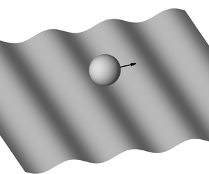
Figure 1 illustrates a spherical particle with radius  $a$ moving near a sinusoidal surface $z=A_{max}\cos kx$, where $k=2{\rm \pi} /\lambda$ is the wavenumber, and $\lambda$ is the wavelength. The sphere is positioned at $\boldsymbol {r}_0=(x_0, 0, h)$ and is subjected to a constant force $\boldsymbol {F}$ without any torque. The primary task of this work is to determine the dependence of sphere mobility on $x_0$ and $h$. The hydrodynamic interaction between the sphere and the wall is described by the incompressible Stokes equation
 \begin{equation} -\boldsymbol{\nabla}\boldsymbol{\cdot} \boldsymbol{\sigma}=0,\quad \boldsymbol{\nabla}\boldsymbol{\cdot}\boldsymbol{u}=0, \end{equation}
where  $\boldsymbol {\sigma }=p\boldsymbol{\mathsf{I}}+\mu \boldsymbol {\nabla }(\boldsymbol {u}+\boldsymbol {u}^\textrm {T})$ is the fluid stress tensor, $p$ is the pressure, $\boldsymbol {u}$ is the fluid velocity, $\boldsymbol{\mathsf{I}}$ is the identity matrix and $\mu$ is the fluid viscosity. The boundary conditions for the fluid flow are
 $$\begin{gather} \boldsymbol{u}=\boldsymbol{U}+\boldsymbol{r}\times\boldsymbol{\varOmega},\quad \textrm{on}\ S_p, \end{gather}$$
 $$\begin{gather}\boldsymbol{u}=\boldsymbol{0},\quad \textrm{on}\ S_w\ \textrm{and}\ S_\infty, \end{gather}$$
where  $\boldsymbol {U}$ and $\boldsymbol {\varOmega }$ are the translational and rotational velocities of the sphere, $S_p, S_w$ and $S_\infty$ represent the sphere's surface, the curved wall and the bounding surface at infinity, respectively. The sphere velocity is determined by satisfying the force and torque balancing condition,
 \begin{equation} \int_{S_p}\boldsymbol{n}\boldsymbol{\cdot}\boldsymbol{\sigma}\,{\rm d} S+\boldsymbol{F}=0,\quad \int_{S_p}\boldsymbol{r}\times(\boldsymbol{n}\boldsymbol{\cdot}\boldsymbol{\sigma})\,{\rm d} S=0, \end{equation}
where  $\boldsymbol {n}$ denotes the unit normal vector pointing into the fluid on the sphere's surface. In the following sections, we will solve the above equations using theoretical and numerical methods for curved surfaces with small and arbitrary amplitudes, respectively.

Figure 1. Schematic of the sphere moving near a sinusoidal surface. In the numerical simulation, half of the region is considered and the surface area is  $200a\times 100a$ with a locally refined mesh in the gap between the surface and sphere.
3. Small-amplitude asymptotics
This section presents the theoretical analysis of a sphere's mobility matrix near a sinusoidal surface with small-amplitude fluctuations. The analysis follows the approach from Kurzthaler & Stone (Reference Kurzthaler and Stone2021), which used small-amplitude asymptotics and the Lorentz reciprocal theorem to solve for the roughness-induced velocity of a point swimmer. Considering a curved wall  $z=A(x,y)$ with small amplitude compared with its wavelength, we introduce a small parameter $\varepsilon =A_{max}k\ll 1$, where $A_{max}=\max (|A(x,y)|)$ is the maximum absolute roughness of the surface. Applying the method of domain perturbation, the fluid velocity is expanded as
 \begin{equation} \boldsymbol{u}=\boldsymbol{u}^{(0)}+\varepsilon\boldsymbol{u}^{(1)}+O(\varepsilon^2), \end{equation}
where  $\boldsymbol {u}^{(0)}$ and $\boldsymbol {u}^{(1)}$ are the $O(1)$ and $O(\varepsilon )$ fluid velocities. Substituting the above expansion into (2.1) and (2.2), the governing equations of each order remain as the Stokes equation, while the boundary condition on the curved surface $S_w$ is expanded as
 \begin{equation} \boldsymbol{u}|_{z=A(x,y)}=\boldsymbol{u}^{(0)}|_{z=0} +\varepsilon\left.\left(\boldsymbol{u}^{(1)}+Z(x,y) \frac{\partial\boldsymbol{u}^{(0)}}{\partial z}\right)\right|_{z=0}+O(\varepsilon^2), \end{equation}
where  $Z(x,y)=A(x,y)/(A_{max}k)$ is the rescaled surface height. The right-hand side of the above equation corresponds to the $O(1)$ and $O(\varepsilon )$ boundary conditions, which respectively represent a no-slip condition at the plane wall and a slip velocity condition at $z=0$ due to the surface corrugation. One can then solve the governing equation of each order with the corresponding boundary conditions. The zeroth-order solution $\boldsymbol {u}^{(0)}$, which describes the sphere motion near a plane wall, can be found in the literature using methods of bipolar harmonics or near-contact/far-field asymptotic analyses (O'Neill Reference O'Neill1964; Goldman et al. Reference Goldman, Cox and Brenner1967; O'Neill & Stewartson Reference O'Neill and Stewartson1967; Happel & Brenner Reference Happel and Brenner2012). On the other hand, the first-order velocity $\boldsymbol {u}^{(1)}$, which represents the velocity induced by the surface roughness, does not require explicit solution. Instead, we can apply the reciprocal theorem to the $\boldsymbol {u}^{(0)}$ field to directly find the sphere mobility. The reciprocal theorem has been widely used in the studies of the motion of inert and active particles under the influence of surface confinement, non-Newtonian fluids and external forces (Stone & Samuel Reference Stone and Samuel1996; Elfring Reference Elfring2017; Li & Koch Reference Li and Koch2020). A comprehensive review of its diverse applications in fluid dynamics can be found in Masoud & Stone (Reference Masoud and Stone2019).
To utilize the Lorentz reciprocal theorem, we need to set up an auxiliary problem with known solutions. For our purpose, the auxiliary problem represents the flow field caused by an externally driven, translating or rotating sphere with the same distance  $h$ away from a plane wall. Its solution corresponds to the $\boldsymbol {u}^{(0)}$ velocity field as the original problem. The sphere velocities $\boldsymbol {U}^{(1)}$ and $\boldsymbol {\varOmega }^{(1)}$ are connected to the auxiliary problem as follows:
 \begin{equation} \hat{\boldsymbol{F}}\boldsymbol{\cdot}\boldsymbol{U}^{(1)} +\hat{\boldsymbol{T}}\boldsymbol{\cdot}\boldsymbol{\varOmega}^{(1)}= \int_{z=0}Z(x,y)\left.\left((\boldsymbol{n}\boldsymbol{\cdot}\hat{\boldsymbol{\sigma}}) \boldsymbol{\cdot}\frac{\partial\boldsymbol{u}^{(0)}}{\partial z}\right)\right|_{z=0}{\rm d} S, \end{equation}
where the symbol  $\hat {}$ represents the auxiliary problem, $\hat {\boldsymbol {F}}$ and $\hat {\boldsymbol {T}}$ are the force and torque exerted on the particle. Note that the integration is performed on the plane wall at $z=0$. This equation is valid for arbitrary surface topography and particle–wall distance as long as the surface fluctuation is small.
The translational and rotational velocities of the sphere are related to the force  $\boldsymbol {F}$ and torque $\boldsymbol {\varOmega }$ by a symmetric positive–definite mobility matrix $\boldsymbol{\mathsf{M}}$
 \begin{equation} \begin{pmatrix} \boldsymbol{U}\\ \boldsymbol{\varOmega} \end{pmatrix} = \boldsymbol{\mathsf{M}}\boldsymbol{\cdot} \begin{pmatrix} \boldsymbol{F}\\ \boldsymbol{T} \end{pmatrix}, \end{equation}
where  $\boldsymbol {U}=(U_x,U_y,U_z)^{{\rm T}}$, and similarly for $\boldsymbol {\varOmega }, \boldsymbol {F}$ and $\boldsymbol {T}$. The mobility matrix of a sphere near a corrugated wall with a small amplitude is expanded as
 \begin{equation} \boldsymbol{\mathsf{M}}=\boldsymbol{\mathsf{M}}^{(0)}+\varepsilon\boldsymbol{\mathsf{M}}^{(1)}. \end{equation}
In the following, the mobility matrix of a sphere under both far-field and near-contact conditions will be analysed separately.
The leading-order mobility matrix  $\boldsymbol{\mathsf{M}}^{(0)}$ accounts for the hydrodynamic interaction between a sphere and a plane wall
 \begin{equation} \boldsymbol{\mathsf{M}}^{(0)} = \begin{pmatrix} \textit{M}_{11}^{(0)} & {\cdot} & {\cdot} & {\cdot} & \textit{M}_{15}^{(0)} & {\cdot} \\ {\cdot} & \textit{M}_{22}^{(0)} & {\cdot} & \textit{M}_{24}^{(0)} & {\cdot} & {\cdot} \\ {\cdot} & {\cdot} & \textit{M}_{33}^{(0)} & {\cdot} & {\cdot} & {\cdot} \\ {\cdot} & \textit{M}_{24}^{(0)} & {\cdot} & \textit{M}_{44}^{(0)} & {\cdot} & {\cdot} \\ \textit{M}_{15}^{(0)} & {\cdot} & {\cdot} & {\cdot} & \textit{M}_{55}^{(0)} & {\cdot} \\ {\cdot} & {\cdot} & {\cdot} & {\cdot} & {\cdot} & \textit{M}_{66}^{(0)} \end{pmatrix}, \end{equation}
where the dots represent the identically zero terms because of the symmetry of the sphere-plane configuration.
When the sphere is far away from the wall, i.e.  $a/h\ll 1$, its mobility factors are
 \begin{equation} \left.\begin{gathered} \textit{M}_{11}^{(0)}=\textit{M}_{22}^{(0)} \simeq\frac{1}{6{\rm \pi}\mu a}\left(1-\frac{9a}{16h}\right), \quad \textit{M}_{33}^{(0)}\simeq\frac{1}{6{\rm \pi}\mu a}\left(1-\frac{9a}{8h}\right), \\ \textit{M}_{44}^{(0)}=\textit{M}_{55}^{(0)} \simeq\frac{1}{8{\rm \pi}\mu a^3}\left(1-\frac{5}{16} \left(\frac{a}{h}\right)^3\right), \quad \textit{M}_{66}^{(0)}\simeq\frac{1}{8{\rm \pi}\mu a^3} \left(1-\frac{1}{8}\left(\frac{a}{h}\right)^3\right),\\ \textit{M}_{15}^{(0)}=-\textit{M}_{24}^{(0)} \simeq\frac{1}{64{\rm \pi}\mu a^2}\left(\frac{a}{h}\right)^4 \left(1-\frac{15a}{16h}\right). \end{gathered}\right\} \end{equation}
 When the sphere is in near contact with the wall, i.e.  $\delta =(h-a-A(x,y))/a\ll 1$, the mobility factors are
 \begin{equation} \left.\begin{gathered} \textit{M}_{11}^{(0)}=\textit{M}_{22}^{(0)} \simeq\frac{1}{6{\rm \pi}\mu a}\left(-\frac{2}{\ln\delta}-\frac{4.4678}{(\ln\delta)^2}\right), \quad \textit{M}_{33}^{(0)}\simeq\frac{1}{6{\rm \pi}\mu a} \left(\delta+\frac{1}{5}\delta^2\ln\delta\right), \\ \textit{M}_{44}^{(0)}=\textit{M}_{55}^{(0)} \simeq\frac{1}{8{\rm \pi}\mu a^3}\left(-\frac{8}{3\ln\delta}-\frac{3.7077}{(\ln\delta)^2}\right), \quad \textit{M}_{66}^{(0)}\simeq\frac{1}{8{\rm \pi}\mu a^3}\frac{1}{\zeta(3)},\\ \textit{M}_{15}^{(0)}=-\textit{M}_{24}^{(0)} \simeq\frac{1}{8{\rm \pi}\mu a^2}\left(-\frac{2}{3\ln\delta}-\frac{3.3888}{(\ln\delta)^2}\right), \end{gathered}\right\} \end{equation}
where  $\zeta (3)=\sum _{n=1}^{\infty }n^{-3}=1.20205$. These results are scattered across numerous previous studies, which analysed sphere translation (Brenner Reference Brenner1961; Maude Reference Maude1961) and rotation (Jeffery Reference Jeffery1915; Brenner Reference Brenner1962) perpendicular to the wall at a far distance, sphere motion parallel to the wall at a far distance (Maude Reference Maude1963) and the near-contact motion of a sphere parallel (Goldman et al. Reference Goldman, Cox and Brenner1967; O'Neill & Stewartson Reference O'Neill and Stewartson1967) and perpendicular (Cox & Brenner Reference Cox and Brenner1967; Cooley & O'Neill Reference Cooley and O'Neill1969) to the wall. A comprehensive summary of the resistance matrix for different gap distances between a sphere and a plane can be found in Falade & Brenner (Reference Falade and Brenner1988). In (3.8), the convergence of the leading-order terms to zero is slow due to the logarithmic dependence on $1/\ln \delta$, and to enhance accuracy, next-order corrections are often included by numerically fitting the coefficients.
From the symmetry of the sphere-wall configuration, it is straightforward to find that the O( $\varepsilon$) mobility matrix should satisfy
 \begin{equation} \boldsymbol{\mathsf{M}}^{(1)} = \begin{pmatrix} \textit{M}_{11}^{(1)} & {\cdot} & \textit{M}_{13}^{(1)} & {\cdot} & \textit{M}_{15}^{(1)} & {\cdot} \\ {\cdot} & \textit{M}_{22}^{(1)} & {\cdot} & \textit{M}_{24}^{(1)} & {\cdot} & \textit{M}_{26}^{(1)} \\ \textit{M}_{31}^{(1)} & {\cdot} & \textit{M}_{33}^{(1)} & {\cdot} & \textit{M}_{35}^{(1)} & {\cdot} \\ {\cdot} & \textit{M}_{42}^{(1)} & {\cdot} & \textit{M}_{44}^{(1)} & {\cdot} & \textit{M}_{46}^{(1)} \\ \textit{M}_{51}^{(1)} & {\cdot} & \textit{M}_{53}^{(1)} & {\cdot} & \textit{M}_{55}^{(1)} & {\cdot} \\ {\cdot} & \textit{M}_{62}^{(1)} & {\cdot} & \textit{M}_{64}^{(1)} & {\cdot} & \textit{M}_{66}^{(1)} \end{pmatrix}. \end{equation}
Each row in the matrix can be calculated by separately applying a force or torque along the  $x$-,
$x$-,  $y$- or $z$-directions in (3.3), the coefficient is found to be
 \begin{equation} \textit{M}_{ij}^{(1)}=\textit{M}_{ji}^{(1)}= \frac{1}{k}\int_{-\infty}^{\infty}m_{ij}^{(1)}\cos k(x+x_0)\,{{\rm d}\kern0.7pt x}, \end{equation}
where
 \begin{equation} m_{ij}^{(1)}=\int_{y=-\infty}^{\infty}\left.\left(\hat{\sigma}_{jz} \frac{\partial u^{(0)}_i}{\partial z}\right)\right|_{z=0}{{\rm d}y}, \end{equation}
and  $\hat {\sigma }_{jz}$ and $\partial u^{(0)}_i/\partial z$ represent the hydrodynamic stresses and velocity gradients at $z=0$. The subscripts $i, j=1,2,3$ correspond to the cases where the sphere motion is driven by a force along the $x$-,
$x$-,  $y$- and $z$-directions, respectively. For $i, j=4,5,6$, the solution represents the sphere motion driven by a torque. The detailed derivation of each coefficient is provided in Appendix A. Equation (3.10) indicates that the influence of a small-amplitude curved surface on particle mobility is simply a linear combination of individual surface areas.
In the far-field approximation, the fluid velocity can be simplified as being generated by a Stokeslet. The coefficients in the above equation are
 \begin{equation} \left.\begin{gathered} m_{11}^{(1)}=-\frac{45}{\varDelta}h^2x^2(8x^2+h^2),\quad m_{22}^{(1)}=-\frac{9}{\varDelta}h^2(x^2+h^2)(8x^2+3h^2), \\ m_{33}^{(1)}=-\frac{45}{\varDelta}h^4(8x^2+h^2), \quad m_{44}^{(1)}=-\frac{9}{4\varDelta}(8x^4+x^2h^2+28h^4), \\ m_{55}^{(1)}=-\frac{45}{4\varDelta}(8x^4-13x^2h^2+7h^4),\quad m_{66}^{(1)}=-\frac{45}{4\varDelta}h^2(8x^2+h^2), \\ m_{13}^{(1)}= \frac{45}{\varDelta}h^3x(8x^2+h^2),\quad m_{15}^{(1)}=-\frac{45}{\varDelta}hx^2(4x^2-3h^2), \\ m_{24}^{(1)}= \frac{9}{\varDelta}h(x^2+h^2)(4x^2-h^2),\quad m_{26}^{(1)}= 0,\\ m_{35}^{(1)}= \frac{45}{\varDelta}h^2x(4x^2-3h^2),\quad m_{46}^{(1)}=-\frac{315}{4\varDelta}h^3x, \end{gathered}\right\} \end{equation}
where  $\varDelta =512{\rm \pi} \mu (x^2+h^2)^{9/2}$. If we further assume that the distance between the sphere and the wall is small compared with the wavelength, i.e. $kh\ll 1$, the mobility factors can be explicitly solved as
 \begin{equation} \left.\begin{gathered} \textit{M}_{11}^{(1)}=\frac{3a(-8+9h^2k^2)C_k}{256h^2{\rm \pi}\mu}, \quad \textit{M}_{22}^{(1)}=\frac{3a(-8+3h^2k^2)C_k}{256h^2{\rm \pi}\mu}, \\ \textit{M}_{33}^{(1)}=\frac{3a(-4+h^2k^2)C_k}{64h^2{\rm \pi}\mu}, \quad \textit{M}_{44}^{(1)}=\frac{15a(-8+h^2k^2)C_k}{1024{\rm \pi}\mu h^4}, \\ \textit{M}_{55}^{(1)}=\frac{3a(-40+7h^2k^2)C_k}{1024{\rm \pi}\mu h^4}, \quad \textit{M}_{66}^{(1)}=\frac{3a(-4+h^2k^2)C_k}{256{\rm \pi}\mu h^4}, \\ \textit{M}_{13}^{(1)}=-\frac{3akS_k}{32{\rm \pi}\mu h}, \quad \textit{M}_{15}^{(1)}=\frac{9ak^2C_k}{256{\rm \pi}\mu h}, \quad \textit{M}_{35}^{(1)}=0, \\ \textit{M}_{24}^{(1)}=-\frac{3ak^2C_k}{256{\rm \pi}\mu h}, \quad \textit{M}_{26}^{(1)}=0, \quad \textit{M}_{46}^{(1)}=\frac{3akS_k}{128{\rm \pi}\mu h^3}, \end{gathered}\right\} \end{equation}
where  $C_k=\cos kx_0$ and $S_k=\sin kx_0$ are used for brevity. This result is valid for arbitrary wavelengths of the wall. The diagonal coefficients $\textit {M}_{11}^{(1)}, \textit {M}_{22}^{(1)}, \ldots, \textit {M}_{66}^{(1)}$ consist of two terms in the numerators. The first term is caused by the variation in distance between the sphere and the wall, while the second term is attributed to wall curvature. This result is consistent with Falade & Brenner (Reference Falade and Brenner1988), where the resistance coefficients of a sphere near a curved wall were derived under the assumption of small wall curvature, i.e. $A_{max}hk^2\ll 1$ for a sinusoidal surface. For the cross-coupling terms, the ones with $k^2\cos kx_0$ indicate the effects caused by the wall curvature, while the terms with $k\sin kx_0$ denote the effects due to the surface slope. Falade & Brenner (Reference Falade and Brenner1988) derived $\textit {M}_{13}^{(1)}=\textit {M}_{46}^{(1)}=0$ and cannot predict the transverse migration and rotation of a sphere induced by a curved wall.
In the near-contact limit,  $\delta =(h-a-A(x,y))/a\ll 1$, solving the motion of a sphere near a curved wall with arbitrary wavelength is challenging because the sphere may collide with multiple points on the surface simultaneously. To avoid this situation, we focus on the cases where the surface has a small curvature $A_{max}hk^2\ll 1$, similar to the work of Falade & Brenner (Reference Falade and Brenner1988). The lubrication-theory solutions for a sphere moving close to a flat plane (Cox & Brenner Reference Cox and Brenner1967; Goldman et al. Reference Goldman, Cox and Brenner1967; O'Neill & Stewartson Reference O'Neill and Stewartson1967; Cooley & O'Neill Reference Cooley and O'Neill1969) can be employed to solve the $O(\varepsilon )$ mobilities by (3.3). However, to simplify the calculation, here, we utilize the solution of Falade & Brenner (Reference Falade and Brenner1988) and calculate the mobility matrix by directly inverting the resistance matrix, $\boldsymbol{\mathsf{M}}=\boldsymbol{\mathsf{R}}^{-1}$. The $O(\varepsilon )$ mobility coefficients are
 \begin{align} \left.\begin{gathered} \textit{M}_{11}^{(1)}=\frac{ak^2C_k}{6{\rm \pi}\mu} \left(-\frac{201}{50\ln\delta}-\frac{3.02001}{(\ln\delta)^2}\right), \quad \textit{M}_{22}^{(1)}=\frac{ak^2C_k}{6{\rm \pi}\mu} \left(-\frac{99}{50\ln\delta}-\frac{13.5478}{(\ln\delta)^2}\right), \\ \textit{M}_{33}^{(1)}=\frac{ak^2C_k}{6{\rm \pi}\mu} \left(\delta+0.2001\delta^{3/2}\right), \quad \textit{M}_{44}^{(1)}=\frac{k^2C_k}{8{\rm \pi}\mu a} \left(-\frac{66}{25\ln\delta}-\frac{17.1254}{(\ln\delta)^2}\right), \\ \textit{M}_{55}^{(1)}=\frac{k^2C_k}{8{\rm \pi}\mu a} \left(-\frac{34}{25\ln\delta}-\frac{5.66758}{(\ln\delta)^2}\right), \quad \textit{M}_{66}^{(1)}=\frac{0.124286k^2C_k}{8{\rm \pi}\mu a}, \\ \textit{M}_{15}^{(1)}=\frac{k^2C_k}{8{\rm \pi}\mu} \left(-\frac{41}{25\ln\delta}-\frac{5.22177}{(\ln\delta)^2}\right), \quad \textit{M}_{24}^{(1)}=\frac{k^2C_k}{8{\rm \pi}\mu} \left(\frac{59}{25\ln\delta}+\frac{17.6088}{(\ln\delta)^2}\right). \end{gathered}\right\} \end{align}
These terms represent the first-order contribution of the wall curvature  ${\sim }k^2\cos kx_0$ to the sphere motion due to the lubrication effects. Detailed information regarding $\boldsymbol{\mathsf{R}}$ for a sphere near a wall with small curvature, as well as the derivation of $\boldsymbol{\mathsf{M}}$, is provided in Appendix B.
Figure 2 shows the effects of the surface wavelength on the particle mobility near a sinusoidal surface under far-field hydrodynamic interaction. The results are normalized by the sphere's mobility  $\textit {M}_0=1/(6{\rm \pi} \mu a)$ (or $\textit {M}_0/a$ for the cross-coupling terms) in an unbounded fluid. The three rows, from top to bottom, represent the translational and angular velocities of the sphere driven by a force in the $x$-,
$x$-,  $y$- and $z$-directions, respectively. For $\lambda /h\ll 1$, the effects of the surface roughness smear out and all $O(\varepsilon )$ velocities reduce to zero. For $\lambda /h\gg 1$, the sphere moves near a local flat plane at a new distance $h-\varepsilon \cos kx_0$, thereby $U_x^{(1)}\simeq -9a\cos kx_0/16h^2$, $U_z^{(1)}$ and $\varOmega _y^{(1)}$ approach zero. At intermediate wavelengths, the surface roughness generates a non-trivial impact on particle motion, even when considering only the far-field hydrodynamics. In figure 2(a), the local hill/valley of the wave tends to decrease/increase the horizontal velocity of the particle for $\lambda /h<0.9352$ and $\lambda /h>4.3192$, while, at an intermediate wavelength, the surface wave causes the opposite effects. Similar behaviour is also observed for roughness-induced particle rotation in figure 2(c). At the leading order, the sphere rotates in a direction as if it were rolling on the wall. The surface roughness with a large wavelength ( $\lambda /h>1.8405$) tends to enhance/impede the particle rotation by decreasing/increasing the effective distance. While at a small wavelength, the trend is the opposite. This is because the edges of the surface valley cause a reflection of the flow field and change the flow direction (Pozrikidis Reference Pozrikidis1987). Figure 2(b) shows the leading-order vertical migration velocity $U_z^{(1)}$ since $U_z^{(0)}=0$. At $0\leq x_0/\lambda \leq 0.5$, $U_z^{(1)}$ is always negative for $\lambda /h>1.2082$ and positive for $\lambda /h<1.2082$, suggesting that the particle trajectory may follow the same or opposite phase of the sinusoidal wave, depending on the surface wavelength. This non-monotonic dependence of sphere mobility on the surface wavelength, which is not captured by the solution of Falade & Brenner (Reference Falade and Brenner1988), has potential applications for separating small particles and cells using surfaces with designed topography. It is important to note that the distance $h$ only affects the magnitude of the $O(\varepsilon )$ mobility, but does not change the critical value of $\lambda /h$ at which the $O(\varepsilon )$ mobility changes sign.

Figure 2. Normalized  $O(\varepsilon )$ mobility coefficients of a sphere at different distances away from a sinusoidal surface; $\textit {M}_0=1/(6{\rm \pi} \mu a)$ is the sphere's translational mobility in an unbounded fluid. Symbols represent the results of Falade & Brenner (Reference Falade and Brenner1988) for $x_0/\lambda =0$.
Figures 2(d) and 2(e) show the particle mobility under a force transverse to the wave direction. Because of the symmetry of the sphere-surface configuration, the particle motion along the grooves of the sinusoidal wall cannot produce a velocity perpendicular to the wall. For  $\lambda /h\ll 1$ or $\lambda /h\gg 1$, the sinusoidal surface approaches a flat plane and the sphere velocity is isotropic inside the plane parallel to the wall. The particle velocity decreases/increases near the hill/valley of the surface for $\lambda /h>1.2082$, and this effect is reversed for $\lambda /h<1.2082$ with a much weaker influence. This result is different from $U_x^{(1)}$, highlighting the anisotropy of the in-plane mobility of a sphere near a sinusoidal surface with an intermediate wavelength. For $\varOmega _x^{(1)}$, its direction is independent of the wavelength. The angular velocity is always enhanced/reduced as the surface roughness decreases/increases the gap distance, which differs from the $\varOmega _y^{(1)}$ in figure 2(c). In the far-field analysis, $\varOmega _z^{(1)}$ is predicted to be zero. However, as we will see later, this is not true when the higher-order hydrodynamic effects are considered.
The third row shows the sphere mobility driven by a force perpendicular to the wall. Figure 2(f) is identical to figure 2(b) due to the symmetry of the mobility matrix. For  $\lambda /h>1.2082$, the particle is horizontally attracted to the hill of the wave, while for $\lambda /h<1.2082$, it is attracted to the valley. In figure 2(g), the vertical motion of the particle is enhanced/impeded when the gap distance is increased/decreased by the surface roughness of $\lambda /h>1.7416$. The particle velocity approaches $U_z^{(1)}\simeq -9\cos kx_0/8h^2$ as the wavelength increases. For $\lambda /h<1.7416$, the direction of $U_z^{(1)}$ is reversed. Figure 2(h) shows that the angular velocity $\varOmega _y^{(1)}$ is always positive, meaning that the far-field effect drives the particle to rotate in the opposite direction compared with the rolling-type rotation of a sphere settling in parallel to a vertical wall. This effect is not predicted by the small-curvature analysis (Falade & Brenner Reference Falade and Brenner1988).
To further explain the non-monotonic dependence of particle mobility on the wavelength, figure 3 compares the  $O(\varepsilon )$ mobility contribution of different segments of the sinusoidal surface. Here, we focus on the translational movement. The mobility contribution of each surface segment is determined by integrating (3.10) over the corresponding range of $x$. The sphere is positioned at $x_0=3\lambda /8$ and $h=5a$, and the surface is divided into a series of inclined surfaces by half of the wavelength. At a small corrugation amplitude, each surface segment independently affects the particle motion. As expected, the surface segments closest to the sphere have the largest impact on particle mobility. The O( $\varepsilon$) mobility due to the entire sinusoidal surface can be effectively approximated by considering only the first three segments closest to the sphere. This approximation becomes less accurate at $\lambda \sim h$. At a large wavelength, the inclined surface $S_1$ directly below the sphere dominates the corrugation-induced mobility. It enhances the diagonal translation mobility by increasing the sphere-surface distance. At intermediate wavelengths, it generates a negative $\textit {M}_{11}^{(1)}$ and reduces the sphere mobility in the $x$-direction. It indicates that the sphere mobility is influenced by both the sphere–wall gap distance and the angle of the inclined surface, which determines the relative importance of the anisotropic mobilities perpendicular and parallel to the surface. In comparison, the surface $S_1$ induces a positive–definite $\textit {M}_{22}^{(1)}$ at all wavelengths, showing that the transverse motion is primarily influenced by the increased gap distance. The surface $S_2$ further increases $\textit {M}_{22}^{(1)}$ due to the increase of the equivalent gap distance from the sphere. For the off-diagonal component, the surface $S_1$ induces a negative–definite $\textit {M}_{13}^{(1)}$. At intermediate wavelengths, $\textit {M}_{13}^{(1)}$ becomes positive mainly due to the influences of $S_2$.

Figure 3. The contribution of different surface segments on the sphere's  $O(\varepsilon )$ translational mobility coefficients, $x_0=3\lambda /8$ and $h=5a$.
The above results are in qualitative agreement with the previous analysis of the far-field interaction of a microswimmer with a corrugated surface (Kurzthaler et al. Reference Kurzthaler, Zhu, Pahlavan and Stone2020). Their study provides the corrugation-induced velocities for higher-order singularities, including force dipole, source dipole, force quadrupole and rotlet dipole, which also show non-monotonic variation with the wavelength. However, limited by the small-amplitude approximation, surface corrugation has weak effects on particle mobility. In the next section, numerical simulations will be performed to study the sphere motion near a large-amplitude surface and stronger effects from the surface corrugation will be observed.
4. Numerical simulation
In this section, the Stokes equation is numerically solved for a sphere moving near a sinusoidal surface using an in-house developed boundary element code. The approach is based on the previous work by Pozrikidis (Reference Pozrikidis2002) and Zhu, Lauga & Brandt (Reference Zhu, Lauga and Brandt2013). Both the sphere and the sinusoidal wall are modelled as rigid solid bodies. The fluid velocity around rigid bodies in an unbounded fluid domain can be represented in the following integral form:
 \begin{equation} \boldsymbol{u}(\boldsymbol{r})=\frac{1}{8{\rm \pi}\mu} \int_{S_p+S_w}\boldsymbol{\mathsf{G}}(\boldsymbol{r}-\boldsymbol{r}') \boldsymbol{\cdot}\boldsymbol{f}(\boldsymbol{r'})\,{\rm d} S', \end{equation}
where  $\boldsymbol{\mathsf{G}}=\boldsymbol{\mathsf{I}}/r+\boldsymbol {r}\boldsymbol {r}/r^3$ is the Green's function for the Stokes flow, $\boldsymbol{\mathsf{I}}$ is the Kronecker delta tensor, $r=\sqrt {\boldsymbol {r}\boldsymbol {\cdot }\boldsymbol {r}}$ is the distance and $\boldsymbol {f}$ is the unknown force acting on the fluid by the discretized surface element. Due to the symmetry of the problem, the current simulation considers only half of the domain ( $\kern0.08em y\leq 0$). The halves of the sphere and surface are discretized using $N_s$ and $N_w$ quadrilateral elements, respectively. On each surface element $S_i$, the unknown element force $\boldsymbol {f}_i$ is assumed to be constant and contributes to the velocity of the solid body by
 \begin{equation} \boldsymbol{u}_j=\frac{1}{8{\rm \pi}\mu}\sum_{i=1}^{N_s+N_w}\boldsymbol{f}_i \int_{S_i}\boldsymbol{\mathsf{G}}(\boldsymbol{r}_j-\boldsymbol{r}_i)\,{\rm d} S, \end{equation}
and leads to  $3(N_s+N_w)$ independent linear equations. For the elements on the wall surface, the velocity $\boldsymbol {u}_j$ is fixed to zero, and for the sphere elements, the velocity is determined by the rigid body motion
 \begin{equation} \boldsymbol{u}_i=\boldsymbol{U}+\boldsymbol{\varOmega}\times(\boldsymbol{r}_i-\boldsymbol{r}_0), \end{equation}
where  $\boldsymbol {U}$ and $\boldsymbol {\varOmega }$ are the unknown translational and rotational velocities, and $\boldsymbol {r}_0$ is the centre of the sphere. The linear system is then closed by 6 extra linear equations satisfying the force and torque balance of the sphere
 \begin{equation} \sum_{i=1}^{N_s}\boldsymbol{f}_i=\boldsymbol{F},\quad \sum_{i=1}^{N_s}(\boldsymbol{r}_i-\boldsymbol{r}_0)\times\boldsymbol{f}_i=\boldsymbol{T}, \end{equation}
where  $\boldsymbol {F}$ and $\boldsymbol {T}$ are the external force and torque applied on the sphere. As the sphere is free of torque, $\boldsymbol {T}$ is set to zero in this study. The $(3N_s+3N_w+6)\times (3N_s+3N_w+6)$ matrix problem is solved for $\boldsymbol {f}_i, \boldsymbol {U}$ and $\boldsymbol {\varOmega }$ using the DGESV function in LAPACK linear algebra library.
To validate the numerical code, the translation of a sphere near a plane wall is first simulated. The analytical and numerical solutions for the drag and torque coefficients of a sphere translating perpendicular or parallel to a plane wall can be found in Goldman et al. (Reference Goldman, Cox and Brenner1967). Quadrilateral elements are used to discretize both the sphere and the surface. Compared with triangular elements, such a method allows a natural parametrization of the edge to facilitate the numerical integration using the Gauss–Legendre quadrature. For singular elements, the simulation is transformed into an integration based on the plane polar coordinate system (Pozrikidis Reference Pozrikidis2002). In this work, the half-sphere and the half-plane are discretized by 3100 and 16 022 elements, respectively. The grids are locally refined in the gap between the sphere and the wall, with the minimum grid  ${\sim }0.008a$. The size of the wall plane is $40a\times 40a$ following Zhu et al. (Reference Zhu, Lauga and Brandt2013). The force and torque coefficients for a sphere moving perpendicular and parallel to the wall are compared against the literature, as shown in table 1. It is verified that the current simulation can accurately replicate the reported results.
Table 1. Comparison between the current simulation and the previous results for a sphere translating near an infinitely large rigid plane wall.

For a sphere moving near a sinusoidal wall, a larger surface of  $200a\times 100a$ is used to accurately capture the hydrodynamic effects of surface corrugation on the sphere motion. The sphere is located above the centre of the surface to minimize the error due to the truncation of the domain. As the sphere approaches the surface, the quadrilateral elements are successively refined by dividing them evenly into four elements in the gap region, ensuring an accurate simulation of the particle motion in both the far field and near field of the sinusoidal wall.
Figure 4 shows the normalized mobilities of the sphere near a sinusoidal surface of  $A=0.1a$. Consistent with previous findings by Spagnolie & Lauga (Reference Spagnolie and Lauga2012), the far-field approximation agrees reasonably well with the numerical results until $h\sim 2a$, after which the far-field analysis results show significant deviation and even show quantitative differences from the simulation. In the near-contact region, all the mobility components eventually reduce to zero as the gap distance decreases to zero. However, due to the $1/\ln \delta$ asymptotes, the sphere still has a relatively large velocity parallel to the wall even when it is in close proximity to the surface. For clarity, the $1/(\ln \delta )^2$ terms in the near-contact asymptotes are not shown here. The three diagonal components monotonically reduce to zero with decreasing $h$, while the off-diagonal terms initially reach a peak close to the wall and then decrease to zero. This trend is not captured by the far-field or lubrication asymptotes and requires extremely fine grid resolution to be fully captured in simulations.

Figure 4. Normalized mobility coefficients of a sphere near a sinusoidal surface with  $\lambda =20a$ and $A=0.1a$; $\textit {M}_0=1/(6{\rm \pi} \mu a)$ is the sphere's translational mobility in an unbounded fluid. Solid lines: numerical results, dashed lines: far-field solution, dotted lines: lubrication solution.
In figures 4(a) and 4(d), the two mobilities  $\textit {M}_{11}$ and $\textit {M}_{22}$ are close to each other because the particle motion is mainly influenced by the same virtual plane wall at $y=0$. The sinusoidal wave affects their relative magnitudes at different horizontal locations (see insets). Figure 4(f) shows that the sphere has a non-zero $\varOmega _z$ when it translates parallel to the grooves of the sinusoidal surface. This effect, which is mainly caused by the hydrodynamic interaction between the sphere and the locally inclined surface, is not captured by the far-field analysis at the leading order. In figure 4(h), the velocity $U_z\sim h$ linearly reduces to zero as the particle approaches the wall. The far-field analysis can predict the same trend, while the quantitative results are not correct. The vertical velocity $U_z$ is significantly different from $U_x$ and $U_y$. The anisotropic translational mobility of a particle perpendicular and parallel to the wall is a key factor for the accumulation of microswimmers near a surface (Berke et al. Reference Berke, Turner, Berg and Lauga2008; Li & Ardekani Reference Li and Ardekani2014). Similar behaviour can also be observed for microswimmers near a corrugated surface (Ishimoto et al. Reference Ishimoto, Gaffney and Smith2021; Kurzthaler & Stone Reference Kurzthaler and Stone2021). Finally, in figure 4(i), the direction of the particle rotation is reversed when the particle–wall distance $h\lesssim 2a$, showing that the near-field hydrodynamic interaction causes the sphere to roll on the surface.
With a larger amplitude, the surface has stronger influences on the sphere mobility. Figure 5 shows the particle motion near a sinusoidal surface with  $A=5a$ and $\lambda =20a$, for which the far-field analysis only qualitatively agrees with the numerical results. Here, for the far-field results, the sphere–wall distance $h$ has subtracted the local surface height directly beneath the centre of the sphere. Surprisingly, this adjustment leads to a better agreement between the far-field and numerical results, especially for $\textit {M}_{51}$ and $\textit {M}_{42}$. In figures 5(c) and 5(e), the translation-induced rotation at a large $h$ is in the same direction as the sphere rolling on the surface. The result is the same as the sphere movement near a surface with a small amplitude. While, at an intermediate distance, the sphere will rotate in the opposite direction for $x_0>\lambda /4$. This effect, which is caused by the strong hydrodynamic interaction between the sphere and a locally curved trough of the surface, can be qualitatively captured by the far-field analysis. Further close to the surface, the particle returns to the rolling-type motion near the surface. Similar behaviour is also shown in figure 5(f), where $\varOmega _z$ at $x=3\lambda /4$ becomes negative at $0\lesssim h\lesssim 5a$. In figure 5(g), the transverse velocity $U_x$ of the sphere is negligible when it is far away from the surface and changes the direction at $h\simeq 21a$. When the sphere is close to the wall, the sinusoidal surface induces a large transverse velocity $U_x$ of comparable magnitude to $U_z$. Since a sphere moving perpendicular to the wall requires a long time to collide with the wall, $U_x$ can cause significant transverse migration of the particle along the wave direction. This effect leads to a strong accumulation of particles at the valley when they settle down towards a corrugated surface.

Figure 5. Normalized mobility coefficients of a sphere near a sinusoidal surface with  $\lambda =20a$ and $A=5a$; $\textit {M}_0=1/(6{\rm \pi} \mu a)$ is the sphere's translational mobility in an unbounded fluid. Solid lines: numerical results, dashed lines: far-field solution, dotted lines: lubrication solution.
To better illustrate the sphere motion near a sinusoidal surface, figure 6 displays the trajectory of a sphere moving near a sinusoidal surface driven by a horizontal and vertical force. The position of the sphere centre is explicitly updated over time using the fourth-order Adams–Bashforth scheme
 \begin{equation} \boldsymbol{r}^{n+1}_0=\boldsymbol{r}^{n}_0+\frac{\Delta t}{24} [55\boldsymbol{U}(\boldsymbol{r}^{n}_0)-59\boldsymbol{U}(\boldsymbol{r}^{n-1}_0) +37\boldsymbol{U}(\boldsymbol{r}^{n-2}_0)-9\boldsymbol{U}(\boldsymbol{r}^{n-3}_0)], \end{equation}
where the subscripts  $n+1, n, n-1, \ldots$ represent different time steps and the step size is set to $\Delta t=0.1$. Lower-order schemes are utilized for the initial time steps. To minimize simulation errors resulting from domain truncation, the sphere is positioned above the centre of the sinusoidal wall. At the $(n+1)$th time step, the discretized wall grids are updated using $z^{n+1}=A_{max}\cos k(x+x_0^n)$, where $x_0^{n+1}$ is the new assigned $x$-location of the sphere centre. In figure 6(a), the sphere exhibits an oscillating trajectory when moving parallel to the surface. The trajectory is flattened when the sphere is moving above the valley of the surface, indicating a strong suppression of the vertical motion due to the inclined walls on both sides. The amplitude of the oscillation increases as the trajectory is closer to the wall and, after one period, the sphere returns to the original height. In the inset of figure 6(a), the sphere close to the wall takes a much longer time to travel from $x_0=0$ to $x_0=\lambda /2$. Figure 6(b) shows the trajectories of a sphere released from the same initial $y$-location $h=10a$ and three different $x$-locations, $x/\lambda =0.25, 0.5, 0.75$. The sphere descends towards the valley of the surface. This effect becomes stronger as the sphere approaches the surface. Eventually, the sphere is nearly in contact with the wall and falls along the surface.

Figure 6. The trajectories of a sphere driven by a force (a) parallel and (b) perpendicular to a sinusoidal surface with  $\lambda =20a$ and $A=5a$. The inset in (a) shows the dependence of the minimum height $h_{min}$ of the sphere on the maximum height $h_{max}$ and the travel time $\Delta T$ from $x_0=0$ to $x_0=\lambda /2$, symbols show the numerical results and lines show the far-field approximate solution.
Finally, we further compare the effects of surface wavelength and amplitude on the mobility of a sphere at a constant distance from the wall. Figure 7(a) shows the translational mobility of a sphere at  $x_0=3\lambda /8$ near a surface with a constant amplitude $A=5a$ and varying wavelengths. When the sphere is at a fixed height $h$ (triangle symbols), all the diagonal mobilities increase monotonically with wavelength, and the off-diagonal mobility $\textit {M}_{13}$ reaches the minimum at $\lambda \simeq 6a$ and then slowly increases. The transverse mobility $\textit {M}_{22}$ is always larger than the longitudinal and vertical mobilities, and the relative strength of $\textit {M}_{11}$ and $\textit {M}_{33}$ is dependent on the wavelength. For a sphere at constant gap distance from the surface (square symbols for $d_{min}=1.2a$), $\textit {M}_{22}$ and $\textit {M}_{13}$ are weakly influenced by changing the wavelength, while $\textit {M}_{11}$ and $\textit {M}_{33}$ show stronger dependence on $\lambda$. Figure 7(b) shows qualitatively similar behaviour when changing the surface amplitude. These results demonstrate that the sphere's movement can become complicated by its near-field hydrodynamic interaction with a surface of large corrugation amplitude.

Figure 7. The translational mobility of a sphere at  $x_0=3\lambda /8$ near a sinusoidal surface with (a) constant amplitude $A=5a$ and varying wavelength, and (b) constant wavelength $\lambda =20a$ and varying amplitude; $\textit {M}_0=1/(6{\rm \pi} \mu a)$ is the sphere's translational mobility in an unbounded fluid. Triangles represent the sphere has a fixed vertical position $h=2.39627a$ and $h=0.854141a$ in (a,b), respectively, and squares represent the sphere has a fixed minimum distance $d=1.2a$ from the surface.
5. Conclusion
This work investigates the sphere mobility driven by an external force near a sinusoidal surface in the Stokes regime. For a surface with a small amplitude, solutions of far-field or near-contact approximation are derived using the Lorentz reciprocal theorem. At a large amplitude, the sphere mobility is solved using the boundary element method and shows good agreement with the two asymptotes. Compared with a plane surface, a corrugated surface induces additional translational and rotation velocity components to the particle's movement. The direction of the corrugation-induced velocities is dependent on the wavelength of the surface. The key finding is that, in the far-field regime, a sphere settling perpendicular to a sinusoidal surface tends to slowly migrate towards the hill of the wall while, in the near field, it migrates towards the valley with a large transverse velocity. As the sphere approaches the surface, the magnitude of the transverse velocity becomes comparable to the vertical velocity and can significantly affect the sedimentation process. At an intermediate distance from the wall, the far-field and lubrication theories fail to accurately calculate the sphere mobility, and numerical simulations are necessary to fully capture the hydrodynamics.
Acknowledgements
We would like to thank L. Zhu for the helpful discussion and the anonymous reviewers for their valuable comments in improving this manuscript.
Funding
This research is supported by the National Natural Science Foundation of China (No. 12102258, 12372264) and the Natural Science Foundation of Shanghai (No. 23ZR1430800).
Declaration of interests
The authors report no conflict of interest.
Appendix A. Derivation of the far-field mobility coefficients
When the particle is far away from the surface, the fluid flow can be characterized using the multipole expansion of the fundamental singularities of the Stokes equation. To simplify the expressions, the centre of the sphere is set to  $\boldsymbol {r}_0=0\boldsymbol {e}_x+0\boldsymbol {e}_y+h\boldsymbol {e}_z$, and the wall surface is written as $z=A_{max}\cos k(x+x_0)$. The force acting on the sphere is $\boldsymbol {F}=F(\cos \theta \boldsymbol {e}_\phi +\sin \theta \boldsymbol {e}_z)$, where $F$ is the force magnitude, $\boldsymbol {e}_\phi =\boldsymbol {e}_x\cos \phi +\boldsymbol {e}_y\sin \phi$, $\theta$ is the angle between the $z$-axis and the force direction and $\phi$ is the angle between the $x$-axis and the force projection inside the $x-y$ plane. At the leading order, the velocity field is represented by a combination of a Stokeslet and the image singularities due to the plane wall
 \begin{equation} \boldsymbol{u}^{(0)}(\boldsymbol{r})=\frac{F}{8{\rm \pi}\mu}(\boldsymbol{G} (\boldsymbol{r}-\boldsymbol{r}_0, \boldsymbol{e}) +\boldsymbol{G}^*(\boldsymbol{r}-\boldsymbol{r}_0^*, \boldsymbol{e})). \end{equation}
The first term represents the Stokeslet
 \begin{equation} \boldsymbol{G}(\boldsymbol{r}, \boldsymbol{e})=\frac{1}{|\boldsymbol{r}|} \left(\boldsymbol{e}+\frac{(\boldsymbol{e}\boldsymbol{\cdot}\boldsymbol{r}) \boldsymbol{r}}{|\boldsymbol{r}|^2}\right), \end{equation}
and the second term  $\boldsymbol {G}^*$ represents the image singularities induced by a plane wall
 \begin{equation} \boldsymbol{G}^*(\boldsymbol{r}-\boldsymbol{r}_0^*, \boldsymbol{e})=-\boldsymbol{G}(\boldsymbol{e})+2h\boldsymbol{G}_D(\boldsymbol{e}^*,\boldsymbol{e}_z) -2h^2\boldsymbol{S}_D(\boldsymbol{e}^*), \end{equation}
where  $\boldsymbol {e}^*=\boldsymbol {e}_\phi \cos \theta -\boldsymbol {e}_z\sin \theta, \boldsymbol {r}_0^*=\boldsymbol {r}_0-2h\boldsymbol {e}_z$, and on the right-hand side we use a shorthand notation $\boldsymbol {G}(\boldsymbol {e})=\boldsymbol {G}(\boldsymbol {r}-\boldsymbol {r}_0^*, \boldsymbol {e})$. The three terms represent a Stokeslet, a Stokeslet dipole and a source dipole, respectively. The Stokeslet dipole and the source dipole are derivatives of a Stokeslet $\boldsymbol {G}_D(\boldsymbol {r}-\boldsymbol {r}_0, \boldsymbol {d}, \boldsymbol {e})=\boldsymbol {d}\boldsymbol {\cdot }\boldsymbol {\nabla }_0 \boldsymbol {G}(\boldsymbol {r}-\boldsymbol {r}_0, \boldsymbol {e})$ and $\boldsymbol {S}_D(\boldsymbol {r}-\boldsymbol {r}_0, \boldsymbol {e})=-\nabla _0^2\boldsymbol {G}(\boldsymbol {r}-\boldsymbol {r}_0, \boldsymbol {e})/2$, where $\boldsymbol {\nabla }_0$ represents gradient acting on the singularity position $\boldsymbol {r}_0$, and their expressions are
 $$\begin{gather} \boldsymbol{G}_D(\boldsymbol{r}, \boldsymbol{d}, \boldsymbol{e})=\frac{1}{|\boldsymbol{r}|^2} \left(\frac{(\boldsymbol{d}\boldsymbol{\cdot}\boldsymbol{r}) \boldsymbol{e}-(\boldsymbol{e}\boldsymbol{\cdot}\boldsymbol{r}) \boldsymbol{d}-(\boldsymbol{d}\boldsymbol{\cdot}\boldsymbol{e}) \boldsymbol{r}}{|\boldsymbol{r}|} +\frac{3(\boldsymbol{e}\boldsymbol{\cdot}\boldsymbol{r})(\boldsymbol{d}\boldsymbol{\cdot}\boldsymbol{r}) \boldsymbol{r}}{|\boldsymbol{r}|^3}\right), \end{gather}$$
 $$\begin{gather}\boldsymbol{S}_D(\boldsymbol{r}, \boldsymbol{e})=\frac{1}{|\boldsymbol{r}|^3} \left(-\boldsymbol{e}+\frac{3(\boldsymbol{e}\boldsymbol{\cdot}\boldsymbol{r}) \boldsymbol{r}}{|\boldsymbol{r}|^2}\right). \end{gather}$$
The pressure fields induced by a Stokeslet, a Stokeslet dipole and a source dipole are respectively
 \begin{equation} p_{G}=\frac{2\mu\boldsymbol{r}\boldsymbol{\cdot}\boldsymbol{e}}{|\boldsymbol{r}|^3},\quad p_{GD}=\frac{2\mu}{|\boldsymbol{r}|^3}\left(\frac{3(\boldsymbol{r}\boldsymbol{\cdot} \boldsymbol{e})(\boldsymbol{r}\boldsymbol{\cdot}\boldsymbol{d})}{|\boldsymbol{r}|^2}-\boldsymbol{d}\,{\cdot}\, \boldsymbol{e}\right),\quad p_{SD}=0. \end{equation}
The pressure solution is used to calculate the hydrodynamic stresses for the auxiliary problem.
On the plane surface, the velocity gradients are
 \begin{equation} \left.\begin{gathered} \left.\frac{\partial u^{(0)}_x}{\partial z}\right|_{z=0}= \frac{3xh(x\cos\theta\cos\phi+y\cos\theta\sin\phi-h\sin\theta)}{2{\rm \pi}\mu(h^2+x^2+y^2)^{5/2}},\\ \left.\frac{\partial u^{(0)}_y}{\partial z}\right|_{z=0}= \frac{3yh(x\cos\theta\cos\phi+y\cos\theta\sin\phi-h\sin\theta)}{2{\rm \pi}\mu(h^2+x^2+y^2)^{5/2}}, \end{gathered}\right\} \end{equation}
and  $\partial u^{(0)}_z/\partial z|_{z=0}=0$ by the incompressible condition.
To solve (3.3) using the reciprocal relation, two auxiliary problems are introduced to calculate the influence of the curved surface. The first problem describes a point force near a plane surface, which solution is shown above. The hydrodynamic stresses on the plane surface can be directly calculated as
 \begin{equation} \left.\begin{gathered} \hat{\sigma}_{xz}|_{z=0}=\mu\left.\frac{\partial u^{(0)}_x}{\partial z}\right|_{z=0},\quad \hat{\sigma}_{yz}|_{z=0}=\mu\left.\frac{\partial u^{(0)}_y}{\partial z}\right|_{z=0},\\ \hat{\sigma}_{zz}|_{z=0}=\frac{-3\mu h^2(x\cos\theta\cos\phi+y\cos\theta\sin\phi-h\sin\theta)} {2{\rm \pi}(h^2+x^2+y^2)^{5/2}}. \end{gathered}\right\} \end{equation}
Equations (A7) and (A8) are then substituted into (3.3) to derive the mobility coefficients of a sphere driven by a force near a non-planar surface.
The second auxiliary problem considers the sphere motion driven by a torque. In the leading order, the velocity is represented by a point torque near a plane
 \begin{equation} \boldsymbol{u}^{(0)}(\boldsymbol{r})=\frac{T}{8{\rm \pi}\mu}(\boldsymbol{R} (\boldsymbol{r}-\boldsymbol{r}_0, \boldsymbol{e}) +\boldsymbol{R}^*(\boldsymbol{r}-\boldsymbol{r}_0^*, \boldsymbol{e})), \end{equation}
where the first term represents a rotlet
 \begin{equation} \boldsymbol{R}(\boldsymbol{r}, \boldsymbol{e})=\frac{\boldsymbol{e}\times\boldsymbol{r}}{|\boldsymbol{r}|^3}, \end{equation}
and the second term represents the image singularities
 \begin{equation} \boldsymbol{R}^*(\boldsymbol{r}-\boldsymbol{r}_0^*, \boldsymbol{e})=-\boldsymbol{R}(\boldsymbol{e})+\cos\theta(-\boldsymbol{G}_D(\boldsymbol{e}_z, \boldsymbol{e}_\phi^\perp) -\boldsymbol{G}_D(\boldsymbol{e}_\phi^\perp, \boldsymbol{e}_z) +2h\boldsymbol{S}_D(\boldsymbol{e}_\phi^\perp)), \end{equation}
where  $\boldsymbol {e}_\phi ^\perp =\boldsymbol {e}_z\times \boldsymbol {e}_\phi$, $\boldsymbol {G}_D$ and $\boldsymbol {S}_D$ are the Stokeslet dipole and source dipole. The rotlet does not disturb the pressure field, i.e. $p_R=0$.
On the plane surface, the velocity gradients are
 \begin{equation} \left.\begin{gathered} \left.\frac{\partial u^{(0)}_x}{\partial z}\right|_{z=0}=-\frac{3h(xy\cos\theta\cos\phi+(h^2-x^2)\cos\theta\sin\phi+hy\sin\theta)}{4{\rm \pi}\mu(h^2+x^2+y^2)^{5/2}},\\ \left.\frac{\partial u^{(0)}_y}{\partial z}\right|_{z=0}= \frac{3h(xy\cos\theta\sin\phi+(h^2-y^2)\cos\theta\cos\phi+hx\sin\theta)}{4{\rm \pi}\mu(h^2+x^2+y^2)^{5/2}}, \end{gathered}\right\} \end{equation}
and  $\partial u^{(0)}_z/\partial z|_{z=0}=0$ by the incompressible condition.
The hydrodynamic stresses on the plane surface induced by the rotlet is
 \begin{equation} \left.\begin{gathered} \hat{\sigma}_{xz}|_{z=0}=\mu\left.\frac{\partial u^{(0)}_x}{\partial z}\right|_{z=0},\quad \hat{\sigma}_{yz}|_{z=0}=\mu\left.\frac{\partial u^{(0)}_y}{\partial z}\right|_{z=0},\\ \hat{\sigma}_{zz}|_{z=0}=\frac{3\mu h\cos\theta(y\cos\phi-x\sin\phi)}{2{\rm \pi}(h^2+x^2+y^2)^{5/2}}. \end{gathered}\right\} \end{equation}
 For a surface  $A(x,y)=A_{max}\cos k(x+x_0)$, the rescaled surface height $Z(x,y)=A(x,y)/(A_{max}k)=\cos k(x+x_0)/k$. Substituting the above equations into (3.3), the mobility is written as
 \begin{equation} \textit{M}_{ij}^{(1)}=\frac{1}{k}\int_{x=-\infty}^{\infty}\cos k(x+x_0) \underbrace{\int_{y=-\infty}^{\infty}\left.\left(\hat{\sigma}_{jz} \frac{\partial u^{(0)}_i}{\partial z}\right)\right|_{z=0}{{\rm d}y}}_{m_{ij}^{(1)}}{{\rm d}\kern0.7pt x}, \end{equation}
where  $i, j=1,2,\ldots,6$. For $i, j=1,2,3$, solutions (A7) and (A8) are used to describe the sphere motion driven by a force along the $x$-,
$x$-,  $y$- and $z$-directions, respectively. For $i, j=4,5,6$, solutions (A12) and (A13) are used to describe the sphere motion driven by a torque.
Appendix B. Inversion of the resistance matrix
Falade & Brenner (Reference Falade and Brenner1988) have derived the Stokes resistance of a sphere moving near a curved wall of small curvature. Their analysis requires that  $a\kappa \ll 1$ and $h\kappa \ll 1$, meaning the sphere radius $a$ and the distance $h$ are small compared with the radius of curvature of the wall $1/\kappa$. We have used their results to calculate the mobility matrix. The hydrodynamic force and torque on the sphere are linked to the sphere velocity by
 \begin{equation} \begin{pmatrix} \boldsymbol{F}/6{\rm \pi}\mu a\\ \boldsymbol{T}/8{\rm \pi}\mu a^2 \end{pmatrix} = \boldsymbol{\mathsf{R}}\boldsymbol{\cdot} \begin{pmatrix} \boldsymbol{U}\\ \boldsymbol{\varOmega} \end{pmatrix}, \end{equation}
where the resistance matrix
 \begin{equation} \boldsymbol{\mathsf{R}}= \begin{pmatrix} \boldsymbol{\mathsf{R}}_t & \tfrac{4}{3}\boldsymbol{\mathsf{R}}_c^{{\rm T}}\\ \boldsymbol{\mathsf{R}}_c & \boldsymbol{\mathsf{R}}_r \end{pmatrix}, \end{equation}
and  $\boldsymbol{\mathsf{R}}_t=\boldsymbol{\mathsf{R}}_t^{(0)}+a\kappa \boldsymbol{\mathsf{R}}_t^{(1)}, \boldsymbol{\mathsf{R}}_r=\boldsymbol{\mathsf{R}}_r^{(0)}+a\kappa \boldsymbol{\mathsf{R}}_r^{(1)}$ and $\boldsymbol{\mathsf{R}}_c=\boldsymbol{\mathsf{R}}_c^{(0)}+a\kappa \boldsymbol{\mathsf{R}}_c^{(1)}$ are the force resistance, torque resistance, and the cross-coupling term. Note here the results are expanded in terms of the normalized curvature $a\kappa \ll 1$.
The mobility matrix in (3.4) can be directly calculated from  $\boldsymbol{\mathsf{R}}$,
 \begin{equation} \boldsymbol{\mathsf{M}}= \begin{pmatrix} \tfrac{1}{6{\rm \pi}\mu a}\boldsymbol{\mathsf{I}} & \textbf{0}\\ \textbf{0} & \dfrac{1}{8{\rm \pi}\mu a^2}\boldsymbol{\mathsf{I}} \end{pmatrix}\boldsymbol{\cdot} \begin{pmatrix} \boldsymbol{\mathsf{M}}_t & -\dfrac{4}{3} \boldsymbol{\mathsf{M}}_t\boldsymbol{\cdot}\boldsymbol{\mathsf{R}}_c^{{\rm T}} \boldsymbol{\cdot}\boldsymbol{\mathsf{R}}_r^{-1}\\ -\boldsymbol{\mathsf{M}}_r\boldsymbol{\mathsf{R}}_c \boldsymbol{\cdot}\boldsymbol{\mathsf{R}}_t^{-1} & \boldsymbol{\mathsf{M}}_r \end{pmatrix}, \end{equation}
where  $\boldsymbol{\mathsf{M}}_t$ and $\boldsymbol{\mathsf{M}}_r$ are
 \begin{equation} \boldsymbol{\mathsf{M}}_t=\boldsymbol{\mathsf{R}}_t^{-1}- \tfrac{4}{3}\boldsymbol{\mathsf{R}}_c^{-1}\boldsymbol{\cdot} \boldsymbol{\mathsf{R}}_r(\boldsymbol{\mathsf{R}}_c^{-1})^{{\rm T}},\quad \boldsymbol{\mathsf{M}}_r=\boldsymbol{\mathsf{R}}_r^{-1}-\tfrac{4}{3} (\boldsymbol{\mathsf{R}}_c^{-1})^{{\rm T}}\boldsymbol{\cdot} \boldsymbol{\mathsf{R}}_t\boldsymbol{\mathsf{R}}_c^{-1}. \end{equation}
 The corresponding  $O(1)$ and $O(a\kappa )$ resistance matrices are given by (Falade & Brenner Reference Falade and Brenner1988)
 \begin{align} \left.\begin{gathered} \boldsymbol{\mathsf{R}}_t^{(0)}= \begin{pmatrix} A_0 & 0 & 0 \\ 0 & A_0 & 0 \\ 0 & 0 & B_0 \\ \end{pmatrix},\quad \boldsymbol{\mathsf{R}}_r^{(0)}= \begin{pmatrix} C_0 & 0 & 0 \\ 0 & C_0 & 0 \\ 0 & 0 & D_0 \\ \end{pmatrix},\quad \boldsymbol{\mathsf{R}}_c^{(0)}= \begin{pmatrix} 0 & E_0 & 0 \\ -E_0 & 0 & 0 \\ 0 & 0 & 0 \\ \end{pmatrix},\\ \boldsymbol{\mathsf{R}}_t^{(1)}= \begin{pmatrix} A_1 & 0 & 0 \\ 0 & B_1 & 0 \\ 0 & 0 & C_1 \\ \end{pmatrix},\quad \boldsymbol{\mathsf{R}}_r^{(1)}= \begin{pmatrix} D_1 & 0 & 0 \\ 0 & E_1 & 0 \\ 0 & 0 & F_1 \\ \end{pmatrix},\quad \boldsymbol{\mathsf{R}}_c^{(1)}= \begin{pmatrix} 0 & -G_1 & 0 \\ H_1 & 0 & 0 \\ 0 & 0 & 0 \\ \end{pmatrix}. \end{gathered}\right\} \end{align}
 When the sphere is far away from the surface,  $a/h\ll 1$, the coefficients are
 \begin{gather} A_0=1+\frac{9a}{16h},\quad B_0=1+\frac{9a}{8h},\quad C_0=1+\frac{9a^3}{16h^3},\quad D_0=1+\frac{a^3}{8h^3},\quad E_0=\frac{3a^4}{32h^4}, \end{gather}
 \begin{gather} \left.\begin{gathered} A_1=\frac{81}{128},\quad B_1=\frac{27}{128},\quad C_1=\frac{9}{32},\\ D_1=E_1=F_1=0,\quad G_1=\frac{9a}{128h},\quad H_1=\frac{27a}{128h}. \end{gathered}\right\} \end{gather}
 For a sphere in near-contact with the wall,  $(h-a)/a\ll 1$, the coefficients are
 \begin{gather} \left.\begin{gathered} A_0=-\frac{8}{15}\ln\delta+0.9588,\quad B_0=\frac{1}{\delta}-\frac{1}{5}\ln\delta+0.97128,\\ C_0=-\frac{2}{5}\ln\delta+0.3817,\quad D_0=\zeta(3)-\frac{1}{2}\delta\ln\delta,\quad E_0=-\frac{1}{10}\ln\delta-0.1895, \end{gathered}\right\} \end{gather}
 \begin{gather} \left.\begin{gathered} A_1=-\frac{74}{75}\ln\delta-0.6131,\quad B_1=-\frac{26}{75}\ln\delta-0.2876,\\ C_1=\frac{1}{\delta}-0.2001\delta^{-1/2}-1.5613\ln\delta,\quad D_1=-\frac{13}{50}\ln\delta-0.6283,\\ E_1=-\frac{7}{50}\ln\delta-0.3951,\quad F_1=0.1796-2.2232\delta,\\ G_1=-\frac{19}{100}\ln\delta-0.5266,\quad H_1=-\frac{1}{100}\ln\delta+1.0374. \end{gathered}\right\} \end{gather}
Substituting the above equations into (B3), we can derive the  $O(1)$ and $O(a\kappa )$ mobility coefficients consistent with the current results requiring $A_{max}k\ll 1$ and $kh\ll 1$.


