


1 Introduction
Particle entrainment plays a key role in the earth surface dynamics (erosion, transport and deposition of sediments in the atmosphere and rivers), biological flows and many engineering and industrial processes. A fundamental understanding of these transport mechanisms is therefore relevant to physicists and engineers, with a key role often played by the identification of the threshold conditions for the onset of sediment motion, also known as incipient motion. Despite several attempts to address this problem, it has remained elusive owing to the large number of parameters determining the particle dynamics. In particular, the complexity rises from the fact that the particle entrainment is highly sensitive to the bed surface morphology, particle size and shape, exposure and packing conditions, and, not least, to the intermittent behaviour of turbulence in near-bed flows (Dey & Ali Reference Dey and Ali2018).
In general, sediments moving through a fluid flow experience two types of transport: bed load and suspended load. In bed load transport, the sediments slide, roll and hop (or saltate) along the bed; in suspended load transport, sediment motion away from the bed is sustained by the bulk flow (Bagnold Reference Bagnold1966; Chanson Reference Chanson2004). A first approach to the fundamental understanding of this problem focuses on the simplified problem of the flow-induced dynamics of a single sediment particle, initially resting on a sediment bed.
Among the deterministic approaches proposed, the most widely used parameter to predict the onset of incipient motion originates from the seminal work of Shields (Reference Shields1936). There, it is argued that the incipient motion occurs once a threshold non-dimensional boundary shear stress is exceeded. This non-dimensional number is the so-called Shields parameter  $Sh\equiv \unicode[STIX]{x1D70F}_{0}/((\unicode[STIX]{x1D70C}_{p}-\unicode[STIX]{x1D70C})gD)$, where $\unicode[STIX]{x1D70F}_{0}$ is the boundary shear stress, $\unicode[STIX]{x1D70C}_{p}$ and $\unicode[STIX]{x1D70C}$ are the mass density of the sediments and of the carrying fluid, $g$ is the gravitational acceleration and $D$ the sediment particle diameter. The Shields parameter is based on the time-averaged characteristics of the fluid–solid interaction forces, and is therefore not capable of accounting for the fluctuating forces typically encountered in natural and engineering turbulent flows (Diplas & Dancey Reference Diplas and Dancey2013). The incipient motion of individual sediment particles may be observed when the deterministic bed-load predictor is below the threshold of motion (Kleinhans & van Rijn Reference Kleinhans and van Rijn2002), often identified empirically. Although many have tried to improve the initial idea behind the Shields stress criterion (see e.g. Ling (Reference Ling1995), Zanke (Reference Zanke2003), Vollmer & Kleinhans (Reference Vollmer and Kleinhans2007) and Ali & Dey (Reference Ali and Dey2016)), a distinct threshold has not been established due to the complex interactions between the fluid and the particle bed, a function also of the several parameters characterising the problem.
To overcome these issues, stochastic approaches have been suggested as a viable alternative to estimate the probability of events that exceed the threshold of incipient motion. Cheng & Chiew (Reference Cheng and Chiew1998) presented a theoretical derivation of the pickup probability of sediment entrainment on a hydraulically rough flow by considering the instantaneous streamwise velocity to follow a Gaussian distribution. Wu & Chou (Reference Wu and Chou2003) extended this model by proposing a theoretical formulation for the rolling and lifting probabilities for sediment entrainment in hydraulically smooth and transitional flows. This model accounts for the relation between lift coefficient and particle Reynolds number, and criteria for the modes of particle transport in contact and detachment are obtained by applying the equilibrium of forces and moments. For a given relative particle size, the probability of transport in contact mode increases with increasing Shields stress, until the transition from contact to detachment mode occurs, where it starts to decrease. On the other hand, the probability of transport in detachment mode increases monotonically with an increase of the Shields stress (Dey & Ali Reference Dey and Ali2017).
Another modelling approach uses the concept of force impulse to deal with the bed particle entrainment (see Diplas et al. Reference Diplas, Dancey, Celik, Valyrakis, Greer and Akar2008). In this approach, the conditions for incipient motion are determined not only by the magnitude of the maximum force acting on individual grains, but also by the time interval a force exceeding a certain threshold is applied, all for a given bed material and configuration (Celik, Diplas & Dancey Reference Celik, Diplas and Dancey2014). Celik et al. (Reference Celik, Diplas, Dancey and Valyrakis2010) emphasise that the turbulence-induced impulse must exceed the threshold impulse for the motion to start. In addition to the concept of an impulse-based criterion, energy-based approaches have been suggested to tackle the problem. In this case, the geometrical pocket formed by the bed particles is viewed as a potential well with the gravitational and frictional mechanisms imposing an energy barrier for the sediment particle to fully escape the pocket (see e.g. Lee, Ha & Balachandar (Reference Lee, Ha and Balachandar2012) and Valyrakis, Diplas & Dancey (Reference Valyrakis, Diplas and Dancey2013)).
Other studies have focused on a more phenomenological picture. The idea is that coherent structures, moving from the turbulent boundary layer towards the sediment bed, disrupt the viscous sublayer and impinge directly onto the first layer of grains. The interaction between these structures and the individual sediments results in their entrainment. This hypothesis was first introduced by Sutherland (Reference Sutherland1967), who attributed the (re)suspension mechanism to turbulent bursts. Cleaver & Yates (Reference Cleaver and Yates1973) suggested a two-stage mechanism of resuspension due to turbulent bursting: first a relatively slow movement away from the surface in the viscous sublayer, followed, by a rapid movement into the bulk due to a second burst. The main events considered responsible for incipient motion of sediment particles are related to large negative values of the Reynolds shear stresses: the upward motion of slowly moving-fluid parcels (ejections) and downward inrush of rapidly moving fluid parcels (sweeps). Séchet & Le Guennec (Reference Séchet and Le Guennec1999) argue that the dominant mechanism for particle transport is by ejections, as the time and space-scale characteristics of the particle motion in the period between two jumps are commensurable with the corresponding ejections. Moreover, Ninto & Garcia (Reference Ninto and Garcia1996) measured the instantaneous particle velocities during ejections in both smooth and transitionally rough flows, and showed that the streamwise velocity component tends to be much lower than the local mean flow velocity, while their vertical component tends to be rather intense. These fluctuations are much larger than the local standard deviation of the vertical flow velocity, which would indicate that such particles are responding to rather extreme ejection events. On the other hand, Dey, Sarkar & Solari (Reference Dey, Sarkar and Solari2011) suggested that sweep events with downward advection of the streamwise Reynolds normal stress are prevalent during sediment entrainment. The experiments of Dwivedi, Melville & Shamseldin (Reference Dwivedi, Melville and Shamseldin2010) showed the presence of high vertical and horizontal pressure gradients on the sediment particle during the occurrence of a sweep event. The fact that the contribution from sweep events to the Reynolds stresses near porous media increases (Suga, Mori & Kaneda Reference Suga, Mori and Kaneda2011), strengthens this viewpoint.
The continuous growth in computing power, together with the development of efficient numerical methods, made it possible to study fluid–sediment interactions in turbulent flows. Studies where the ratio of particle size to smallest turbulent structures is small highlight the role of ejections on detachment, or even suspension of these particles (see e.g. Soldati & Marchioli (Reference Soldati and Marchioli2009) and Vinkovic et al. (Reference Vinkovic, Doppler, Lelouvetel and Buffat2011)). For larger particle Reynolds number, interface-resolved approaches are required. Vowinckel et al. (Reference Vowinckel, Jain, Kempe and Fröhlich2016) used interface-resolved simulations to study sediment transport through a loosely packed fixed bed; the authors highlight the erosion mechanism, triggered by collision with already eroded particles (see also Frey & Church (Reference Frey and Church2011)). The study of the collective behaviour of sediment particles and pattern formation in a sediment bed has also become accessible through fully resolved numerical simulations (see e.g. Ji et al. (Reference Ji, Munjiza, Avital, Xu and Williams2014), Kidanemariam and Uhlmann (Reference Kidanemariam and Uhlmann2014), Vowinckel, Kempe & Fröhlich (Reference Vowinckel, Kempe and Fröhlich2014) and Mazzuoli, Kidanemariam & Uhlmann (Reference Mazzuoli, Kidanemariam and Uhlmann2019)).
In this work we investigate the dynamics of a finite-size sediment particle (with diameter  $D\approx 20\unicode[STIX]{x1D708}/u_{\unicode[STIX]{x1D70F}}$, where $u_{\unicode[STIX]{x1D70F}}$ is the bed friction velocity and $\unicode[STIX]{x1D708}$ the fluid viscosity) on a porous bed. We fix the size ratio of particle to smallest turbulent structures, and the ratio of particle inertia to fluid inertia, and vary the relative strength of fluid force to buoyant force. Parameters are chosen to include three distinct modes of sediment transport: suspension, saltation and rolling. We aim to investigate the dynamics of the sediment particle for each case by performing fully resolved numerical simulations, which allow us to explore the flow physics with the three-dimensional and time-resolved insight that is still difficult to achieve in a real experiment.
Our results show that for relatively high values of the Shields parameter,  $Sh$, the dynamics are governed by the balance between fluid forces induced by the mean flow and buoyancy. Conversely, for lower values of the $Sh$ – well below the corresponding critical value for the onset of sediment motion – we observe that the particle motion is solely triggered by extreme, strong sweep events. The associated pressure distribution close to the particle shows a clear and consistent fingerprint: an upstream region of higher-than-mean stagnation pressure (a consequence of an increased streamwise velocity), together with a smaller high-pressure spot close to the contact point of the sediment particle with the bed.
This manuscript is organised as follows. In § 2, we present the governing equations and numerical methodology, together with the flow configuration. The role of the Galileo number and the underlying mechanisms of detachment are discussed in § 3. Finally, a summary of the main findings and conclusions are drawn in § 4.
2 Methodology
2.1 Governing equations
The numerical algorithm solves the Navier–Stokes equations for an incompressible Newtonian fluid with density  $\unicode[STIX]{x1D70C}$ and kinematic viscosity $\unicode[STIX]{x1D708}$,
 $$\begin{eqnarray}\displaystyle & \displaystyle \unicode[STIX]{x1D735}\boldsymbol{\cdot }\boldsymbol{u}=0, & \displaystyle\end{eqnarray}$$
 $$\begin{eqnarray}\displaystyle & \displaystyle \frac{\unicode[STIX]{x2202}\boldsymbol{u}}{\unicode[STIX]{x2202}t}+(\boldsymbol{u}\boldsymbol{\cdot }\unicode[STIX]{x1D735})\boldsymbol{u}=-\frac{\unicode[STIX]{x1D735}(p+p_{e})}{\unicode[STIX]{x1D70C}}+\unicode[STIX]{x1D708}\unicode[STIX]{x1D6FB}^{2}\boldsymbol{u}+\,\boldsymbol{f}, & \displaystyle\end{eqnarray}$$
 where  $\boldsymbol{u}$ is the fluid velocity vector, $p$ the modified fluid pressure (i.e. relative to the local hydrostatic load) and $\unicode[STIX]{x1D735}p_{e}$ a constant pressure gradient that drives the flow. The last term on the right-hand side of (2.2) acts close to the surface of the particles to model their presence and is due to the direct forcing immersed boundary method (IBM) used for the fluid–solid coupling.
The dynamics of the rigid, spherical particles are governed by the Newton–Euler equations for conservation of linear and angular momentum:
 $$\begin{eqnarray}\displaystyle & \displaystyle m_{p}\frac{\text{d}\boldsymbol{u}_{p}}{\text{d}t}=\oint _{\unicode[STIX]{x2202}\unicode[STIX]{x1D6FA}_{p}}\unicode[STIX]{x1D749}\boldsymbol{\cdot }\boldsymbol{n}\,\text{d}A-V_{p}\unicode[STIX]{x1D735}p_{e}+(\unicode[STIX]{x1D70C}_{p}-\unicode[STIX]{x1D70C})V_{p}\boldsymbol{g}+\boldsymbol{F}_{col}, & \displaystyle\end{eqnarray}$$
 $$\begin{eqnarray}\displaystyle & \displaystyle I_{p}\frac{\text{d}\unicode[STIX]{x1D74E}_{p}}{\text{d}t}=\oint _{\unicode[STIX]{x2202}\unicode[STIX]{x1D6FA}_{p}}\boldsymbol{r}\times (\unicode[STIX]{x1D749}\boldsymbol{\cdot }\boldsymbol{n})\,\text{d}A+\boldsymbol{T}_{col}, & \displaystyle\end{eqnarray}$$
 with  $\boldsymbol{u}_{p}$ and $\unicode[STIX]{x1D74E}_{p}$ the particle linear and angular velocity. Here, $m_{p}$, $I_{p}$, $\unicode[STIX]{x1D70C}_{p}$ and $V_{p}$ denote the particle mass, moment-of-inertia, mass density and volume, $\boldsymbol{r}$ is the position vector with respect to the particle centre and $\boldsymbol{n}$ the outward-pointing normal to the particle surface $\unicode[STIX]{x2202}\unicode[STIX]{x1D6FA}_{p}$. The fluid stress tensor is given by $\unicode[STIX]{x1D749}=-p\unicode[STIX]{x1D644}+\unicode[STIX]{x1D708}\unicode[STIX]{x1D70C}(\unicode[STIX]{x1D735}\boldsymbol{u}+\unicode[STIX]{x1D735}\boldsymbol{u}^{\text{T}})$. Finally, $\boldsymbol{g}$ denotes the gravitational acceleration, and $\boldsymbol{F}_{col}$ and $\boldsymbol{T}_{col}$ the force and torque resulting from short-range particle–particle and particle–wall interactions, such as lubrication and collisions.
The sets of equations governing each phase are coupled through a no-slip and no-penetration condition at the particle surface, i.e.
 $$\begin{eqnarray}\boldsymbol{u}|_{\unicode[STIX]{x2202}\unicode[STIX]{x1D6FA}_{p}}=\boldsymbol{u}_{p}+\unicode[STIX]{x1D74E}_{p}\times \boldsymbol{r}.\end{eqnarray}$$
This is achieved by extending a standard Navier–Stokes solver with a direct-forcing IBM, as described below.
2.2 Numerical method
We use the direct forcing IBM developed by Uhlmann (Reference Uhlmann2005) and modified by Breugem (Reference Breugem2012), briefly described hereafter. The Navier–Stokes equations governing the fluid phase are solved on a uniform ( $\unicode[STIX]{x0394}x=\unicode[STIX]{x0394}y=\unicode[STIX]{x0394}z$), staggered, Cartesian grid. The spherical particles are discretised by a set of Lagrangian points, uniformly distributed along their surface. The IBM forcing scheme requires three steps: (i) the fluid prediction velocity is interpolated from the Eulerian to the Lagrangian grid, (ii) the IBM force required for matching the local fluid velocity and the local particle velocity is computed on each Lagrangian grid point and (iii) the resulting IBM force is spread from the Lagrangian to the Eulerian grid. The interpolation and spreading operations are done through the regularised Dirac delta function of Roma, Peskin & Berger (Reference Roma, Peskin and Berger1999), which extends over three grid cells in all coordinate directions. Regularisation of the particle–fluid interface can result in a loss of accuracy. Breugem (Reference Breugem2012) showed that by slightly retracting the Lagrangian grid, second-order accuracy for particle-averaged quantities (e.g. drag) can be attained. Due to the kernel support, the forces obtained from different neighbouring Lagrangian points can be spread to the same Eulerian point, which reduces the accuracy of the forcing. This issue is circumvented by iterating the forcing scheme as proposed by Luo et al. (Reference Luo, Wang, Fan and Cen2007). This multi-direct forcing scheme is particularly relevant in the present set-up, because the kernel’s spreading range for forcing points pertaining to two nearly touching spheres may also partially overlap.
When the distance between two particles or a particle and a wall is smaller than  $\unicode[STIX]{x0394}x$, the IBM fails to resolve the short-range hydrodynamic interactions. The particle dynamics are therefore solved with a subgrid-scale model for short-range interactions, based on canonical lubrication interactions in the Stokes regime, and a soft-sphere model for solid–solid contacts; see Costa et al. (Reference Costa, Boersma, Westerweel and Breugem2015). This model is described below for the sake of clarity.
Unresolved normal lubrication interactions and roughness effects are accounted for by a two-parameter model. For a normalised gap distance  $\unicode[STIX]{x1D700}_{\unicode[STIX]{x0394}x}$ (with $\unicode[STIX]{x1D700}\equiv \unicode[STIX]{x1D6FF}_{ij,n}/R_{p}$, with $\unicode[STIX]{x1D6FF}_{ij,n}$ being the gap distance between particles $i$ and $j$), a lubrication correction force is computed. Here $\unicode[STIX]{x1D700}_{\unicode[STIX]{x0394}x}$ corresponds to the threshold below which the IBM fails to resolve canonical lubrication interactions in the Stokes regime. The closure uses a correction force $\unicode[STIX]{x0394}F_{lub}=-6\unicode[STIX]{x03C0}\unicode[STIX]{x1D707}R_{p}u_{ij,n}(\unicode[STIX]{x1D706}(\unicode[STIX]{x1D700})-\unicode[STIX]{x1D706}(\unicode[STIX]{x1D700}_{\unicode[STIX]{x0394}x}))$, added to the integration of the particle Newton equation (2.3), where $\unicode[STIX]{x1D706}$ is the Stokes amplification factor. Roughness effects are accounted for by making this correction independent of the normalised gap width $\unicode[STIX]{x1D700}$ when this quantity is smaller than a threshold $\unicode[STIX]{x1D700}_{\unicode[STIX]{x1D70E}}$, i.e. $\unicode[STIX]{x0394}F_{lub}\propto u_{ij,n}(\unicode[STIX]{x1D706}(\unicode[STIX]{x1D700}_{\unicode[STIX]{x1D70E}})-\unicode[STIX]{x1D706}(\unicode[STIX]{x1D700}_{\unicode[STIX]{x0394}x}))$, for $0<\unicode[STIX]{x1D700}<\unicode[STIX]{x1D700}_{\unicode[STIX]{x1D70E}}$. This correction is applied until the surfaces undergo actual solid–solid contact; then the soft-sphere collision model takes over.
The soft-sphere collision model computes the normal component of the collision force from the following linear spring–dashpot model:
 $$\begin{eqnarray}\boldsymbol{F}_{ij,n}=-k_{n}\unicode[STIX]{x1D739}_{ij,n}-\unicode[STIX]{x1D702}_{n}\boldsymbol{u}_{ij,n},\end{eqnarray}$$
 where  $\unicode[STIX]{x1D739}_{ij}$ and $\boldsymbol{u}_{ij,n}$ are the gap width and relative particle velocity projected in the line of centres $\boldsymbol{n}_{ij}\equiv (\boldsymbol{x}_{j}-\boldsymbol{x}_{i})/(\Vert \boldsymbol{x}_{j}-\boldsymbol{x}_{i}\Vert )$ where $\boldsymbol{x}_{i/j}$ corresponds to the centroid position of particles $i/j$. The spring and dashpot coefficients are given by
 $$\begin{eqnarray}k_{n}=\frac{m_{e}(\unicode[STIX]{x03C0}^{2}+\ln ^{2}e_{n,d})}{(N\unicode[STIX]{x0394}t)^{2}},\quad \unicode[STIX]{x1D702}_{n}=-\frac{2m_{e}\ln e_{n,d}}{(N\unicode[STIX]{x0394}t)},\end{eqnarray}$$
 where  $e_{n,d}$ is the dry coefficient of restitution and $m_{e}=(m_{i}^{-1}+m_{j}^{-1})^{-1}$ the reduced mass of the particles. Here, $N\unicode[STIX]{x0394}t$ is the collision time, set as a multiple $N$ of the time step of the Navier–Stokes solver, $\unicode[STIX]{x0394}t$. This allows the flow solution to gradually adapt to the sudden changes in particle velocity (Costa et al. Reference Costa, Boersma, Westerweel and Breugem2015; Biegert, Vowinckel & Meiburg Reference Biegert, Vowinckel and Meiburg2017). The model for the tangential component of the collision force uses a similar force formulation, but with a Coulomb friction model for sliding motion
 $$\begin{eqnarray}\boldsymbol{F}_{ij,t}=\min (\Vert k_{t}\unicode[STIX]{x1D739}_{ij,t}+\unicode[STIX]{x1D702}_{t}\boldsymbol{u}_{ij,t}\Vert ,\unicode[STIX]{x1D707}_{c}\Vert \boldsymbol{F}_{ij,n}\Vert )\boldsymbol{t}_{ij},\end{eqnarray}$$
 with  $\boldsymbol{t}\equiv -(k_{t}\unicode[STIX]{x1D739}_{ij,t}+\unicode[STIX]{x1D702}_{t}\boldsymbol{u}_{ij,t})/\Vert k_{t}\unicode[STIX]{x1D739}_{ij,t}+\unicode[STIX]{x1D702}_{t}\boldsymbol{u}_{ij,t}\Vert$. Similarly to the formulation of the normal force, the spring and dashpot coefficients are given by
 $$\begin{eqnarray}k_{t}=\frac{m_{e}(\unicode[STIX]{x03C0}^{2}+\ln ^{2}e_{t,d})}{(N\unicode[STIX]{x0394}t)^{2}},\quad \unicode[STIX]{x1D702}_{t}=-\frac{2m_{e}\ln e_{t,d}}{(N\unicode[STIX]{x0394}t)},\end{eqnarray}$$
 with  $m_{e,t}=(2/7)m_{e}$, where $e_{t,d}$ denotes the dry tangential coefficient of restitution and $\unicode[STIX]{x1D707}_{c}$ is the Coulomb coefficient of sliding friction. We refer to Costa et al. (Reference Costa, Boersma, Westerweel and Breugem2015) for more details.
The overall method has been extensively validated against several benchmark cases, and used to study wall-bounded flows laden with finite-sized particles (see e.g. Lashgari et al. (Reference Lashgari, Picano, Breugem and Brandt2014), Picano, Breugem & Brandt (Reference Picano, Breugem and Brandt2015) and Ardekani et al. (Reference Ardekani, Costa, Breugem and Brandt2016)).

Figure 1. Flow configuration. (a) Shows the whole domain, the moving particle is depicted in orange;  $D$ is the particle diameter, $h$ is the height of fluid section and $h_{b}$ is bed height. (b) Shows a close up of the moving particle and bed configuration. For clarity, only the top layer of the bed is shown. The reference frame adopted here has its origin on the plane tangent to the top layer of particles, and at the streamwise and spanwise position of the centre of the sediment particle.
2.3 Computational set-up
We simulate the dynamics of a single mobile particle in a channel flow, placed on top of a porous bed of fixed spheres, of the same size as the mobile particle (figure 1). Direct numerical simulations (DNS) of fully developed turbulent open channel flow are performed in a domain with dimensions of  $L_{x}\times L_{y}\times L_{z}=40D\times 13D\times 14D$, with $x$,
$x$,  $y$ and $z$ being the streamwise, bed-normal and spanwise directions and $D$ the particle diameter. The fixed bed consists of $2560$ spheres in four layers, arranged in a hexagonal close packing configuration. The particles are resolved with $D/\unicode[STIX]{x0394}x=35$ grid points per particle diameter, which corresponds to an inner-scaled grid spacing of $\unicode[STIX]{x0394}x^{+}=u_{\unicode[STIX]{x1D70F}}\unicode[STIX]{x0394}x/\unicode[STIX]{x1D708}=0.6$, which resolves all flow scales; here, $u_{\unicode[STIX]{x1D70F}}=\sqrt{\unicode[STIX]{x1D70F}_{tot}/\unicode[STIX]{x1D70C}}$ is the friction velocity with $\unicode[STIX]{x1D70F}_{tot}$ the total stress, i.e. the sum of the viscous and the Reynolds stress evaluated at the fluid–porous interface (Breugem, Boersma & Uittenbogaard Reference Breugem, Boersma and Uittenbogaard2006). The flow is periodic in the streamwise and spanwise directions, with no-slip/no-penetration and free-slip/no-penetration boundary conditions imposed at the bottom and top boundaries. A uniform pressure gradient $(\unicode[STIX]{x1D735}p_{e})$ forces the flow such that the bulk fluid velocity $U_{b}$ remains constant. Here the bulk Reynolds number is defined as $Re_{b}=U_{b}h/\unicode[STIX]{x1D708}=3000$, where $h=L_{y}-h_{b}$, and $h_{b}=(\sqrt{6}+1.05)D$ is the bed height.
The moving (non-Brownian) particle has a density ratio  $\unicode[STIX]{x1D70C}_{p}/\unicode[STIX]{x1D70C}=1.05$ (e.g. polystyrene in water (van Hout Reference van Hout2013)), and an inner-scaled diameter $D^{+}=u_{\unicode[STIX]{x1D70F}}D/\unicode[STIX]{x1D708}=21.5$. The initial position of the sediment particle centre with respect to the computational box is $[x_{c},y_{c},z_{c}]=[20.5D,(4\sqrt{6}/3+0.55)D,(4\sqrt{3}+0.5)D]$. The reference frame adopted here is depicted in figure 1. In the present study we vary the Galileo number $Ga\equiv \sqrt{(\unicode[STIX]{x1D70C}_{p}/\unicode[STIX]{x1D70C}-1)gD^{3}}/\unicode[STIX]{x1D708}$, which quantifies the relative importance of gravitational to viscous forces. This is achieved by varying the gravitational acceleration (pointing downward in $y$). An initial set of simulations was performed to seek the Galileo numbers corresponding to the different modes of sediment transport considered. The particle collisional parameters are chosen to be close to what is often measured in collision measurements of rigid spheres: $e_{n,d}=0.97$, $e_{t,d}=0.1$ and $\unicode[STIX]{x1D707}_{s}=0.15$ (see Foerster et al. Reference Foerster, Louge, Chang and Allia1994; Yang & Hunt Reference Yang and Hunt2006). The collision time is set to $N=8$ time steps of the Navier–Stokes solver, corresponding to a collision time of around $0.017h/U_{b}$. Other physical and computational parameters are summarised in table 1.
To obtain the initial turbulent field, the simulations start from laminar Poiseuille flow with a high amplitude disturbance consisting of streamwise counter-rotating vortices to trigger the transition to turbulence efficiently (Henningson & Kim Reference Henningson and Kim1991). The position and rotation of the moving particle are fixed at this stage to allow the turbulent field to develop around the particle. When fully developed turbulence is obtained, the mobile particle is released, i.e. the particle dynamics are governed by (2.3) and (2.4). In the text, time has been normalised by the bulk fluid velocity  $U_{b}$ and the particle diameter $D$, i.e. $tU_{b}/D$ denotes the non-dimensional time.
Table 1. Parameters of the DNS data sets; for all cases  $u_{\unicode[STIX]{x1D70F}}/U_{b}=0.066$ and the corresponding Reynolds number based on the friction velocity is $Re_{\unicode[STIX]{x1D70F}}=Re_{b}u_{\unicode[STIX]{x1D70F}}/U_{b}=198$. $Sh=u_{\unicode[STIX]{x1D70F}}^{2}/[(\unicode[STIX]{x1D70C}_{p}/\unicode[STIX]{x1D70C}-1)gD]$ denotes the Shields parameter, which is proportional to the ratio of fluid force on the particle to the weight of the particle. The critical Shields parameter for this particle Reynolds number is equal to $Sh_{cr}=0.0344$ (see Cao, Pender & Meng Reference Cao, Pender and Meng2006). Here, $N_{ini}$ denotes the number of initial conditions tested for each case and $N_{inc}$ the number of the realisations in which incipient movement is detected.

3 Results
We start by characterising the turbulent flow over the porous bed of spheres. The profiles of averaged Eulerian fluid statistics reported here correspond to mean intrinsic averages. The intrinsic average of a quantity  $\unicode[STIX]{x1D709}$ is computed as
 $$\begin{eqnarray}\langle \unicode[STIX]{x1D709}\rangle (y_{j})=\frac{\displaystyle \mathop{\sum }_{ik,t}\unicode[STIX]{x1D709}_{ijk,t}\unicode[STIX]{x1D6F9}_{ijk,t}}{\displaystyle \mathop{\sum }_{ik,t}\unicode[STIX]{x1D6F9}_{ijk,t}},\end{eqnarray}$$
 where  $\unicode[STIX]{x1D6F9}_{ijk,t}$ is the fluid volume fraction at the grid cell $ijk$ and instant $t$, and $y_{j}$ the wall-normal location of the averaging bin, which extends over the entire domain in the two homogeneous directions. The fluid velocity/pressure fluctuations are defined consistently by subtracting the corresponding fluid intrinsic average from the fluid phase velocity. The mean fluid velocity and the bed-normal velocity fluctuations profiles, normalised by $u_{\unicode[STIX]{x1D70F}}$, are depicted in figure 2. The bed is weakly permeable in this case, with porosity $\unicode[STIX]{x1D716}=0.28$, defined as the volume fraction of voids in the bed, so it behaves similarly to a solid wall as the mean velocity profile is reminiscent of a typical channel-flow profile. Nonetheless, close to the bed, the mean profile is altered by the particle form-induced drag and reaches $U=0$ only below the nominal surface level. This is in agreement with the results of Breugem et al. (Reference Breugem, Boersma and Uittenbogaard2006) and Rosti, Brandt & Pinelli (Reference Rosti, Brandt and Pinelli2018), considering the porosity of the bed in our simulations $(\unicode[STIX]{x1D716}=0.28)$.

Figure 2. (a) Mean streamwise velocity profile and (b) root mean square velocity profiles, normalised by the friction velocity,  $u_{\unicode[STIX]{x1D70F}}$, characterising the turbulent flow over the porous bed. The symbols refer to the DNS data of Kim, Moin & Moser (Reference Kim, Moin and Moser1987) for a smooth wall.
Comparison with the DNS data of Kim et al. (Reference Kim, Moin and Moser1987) for smooth wall, shows slightly larger peaks in the profiles of the velocity fluctuations in the cross-stream direction, while the peak of the streamwise root mean square (r.m.s.) velocity profile near the bed is hardly changing. Breugem et al. (Reference Breugem, Boersma and Uittenbogaard2006) argue that this behaviour can be attributed to the weakening of the wall-blocking and wall-induced viscous effects; increasing the wall porosity, the peak in the streamwise r.m.s. profile decreases and elongated streaky structures weaken, replaced by almost two-dimensional structures. Note that the difference in the normal component between our results (blue line) and those of Kim et al. (Reference Kim, Moin and Moser1987) (blue circles) at a normal location close to  $y/h=1$ is due to the difference in the boundary condition of our simulations for an open (half-)channel flow compared to that of Kim et al. (Reference Kim, Moin and Moser1987) for a channel flow with a top wall.
As the size of the moving particle is small compared to the size of the domain, its presence and its eventual motion does not affect the mean flow statistics and the turbulent flow can be considered to be the same for the different cases, i.e. for the different Galileo numbers investigated.

Figure 3. Two-dimensional projection in the  $x{-}y$ plane of the trajectory of the moving particle for different Galileo numbers. The circles mark the position of the particle with a temporal resolution of $\unicode[STIX]{x0394}tU_{b}/D=2$. The trajectories are displayed until time $tU_{b}/D=83$. The colour indicates the non-dimensional spanwise angular velocity. The red line is fixed on the two-dimensional projection of the particle at beginning of the simulations and changes according to the solid-body rotation of the sediment particle; it therefore depicts the change in the angular position of the particle.
The effect of the Galileo number on the dynamical response of the moving particle on top of the bed is visualised first in order to introduce the classification used in the next subsections. We display in figure 3 the trajectory of the moving particle in the bed-normal  $x\text{-}y$ plane for the different Galileo numbers under investigation. All the cases in the figure use the same turbulent flow field, which resulted in incipient movement in all cases, as initial condition. The figure clearly shows that the streamwise displacement of the moving particle varies significantly with the Galileo number. Note also that the maximum off-plane displacement (i.e. in the spanwise direction and computed as average between the different instances for each case; not shown in the figure) is approximately $5D$ for $Ga25$, around $1D$ for $Ga150$ and less than $0.2D$ for $Ga250$ and $Ga310$. As concerns the bed-normal motion, the particle detaches instantly from the bed as exposed to the turbulent field in the case $Ga25$. The particle spends most of the time detached from the bed and bounces on the bed two times during our simulation, at $x/D\approx 23$ and $28$; at this time, it gains significant angular velocity due to the tangential collision force with the bed. The trajectory pertaining to the case $Ga25$ is very similar to the two-stage lift-off pattern observed in van Hout (Reference van Hout2013). The particle with $Ga150$, see figure 3, experiences a sequence of relatively small excursions and quick returns to the wall. Due to these contacts, the particle has, on average, a higher angular velocity than in the case $Ga25$, as shown by the colour scale. For cases $Ga250$ and $Ga310$, the particle is in contact with the bed for the whole duration of the simulation. Note that the particle angular velocities reveal that in both cases the particles display an intermittent roll/no-roll movement. The duration of the periods of zero velocity is expectedly larger for the case $Ga310$, as the particle travels a smaller distance, $10.5D$, whereas the particle with $Ga250$ moves $32D$ during the same time interval.
For a more detailed analysis of each case, we categorise the cases depending on the contact with the bed; in other words, cases  $Ga25$ and $Ga150$, having no contact and limited contact with the bed, and cases $Ga250$ and $Ga310$, when the particles are long in contact with the bed, will be examined together. For each case, the criterion based on the Shields parameter for predicting the initiation of motion is tested (see table 1). One should note that this parameter emphasises the time-averaged characteristics of the applied fluid forces (Diplas & Dancey Reference Diplas and Dancey2013) and the criterion based on this parameter is currently in use for determining the onset of motion when a significant number of sediment particles are subjected to erosion. Despite this, we use this parameter in our study of a single-particle dynamics to put our results in perspective against this classical criterion. Also, we use the terminologies resuspension, saltation, incipient motion and rolling to address the single-particle dynamics when it resembles that of the transported particles in each of the mentioned modes of sediment transport. Indeed, in a natural flow when the Shields parameter is high enough, a significant bed-load motion and suspension would take place (see e.g Revil-Baudard et al. Reference Revil-Baudard, Chauchat, Hurther and Barraud2015; Berzi & Fraccarollo Reference Berzi and Fraccarollo2016). However, in our study, as we focus on the single-sediment dynamics, the cases labelled as resuspension and saltation would mimic the movement of a sediment particle, which, in a real scenario, would be accompanied by a significant number of other sediments.
3.1 Lower Galileo numbers: resuspension and saltation
We start with cases  $Ga25$ and $Ga150$, when the particle does not remain in contact with the bed. Each of these cases was run with four different turbulent initial conditions. Figure 4 shows the time history of the bed-normal position of the particle centre for all the realisations of case $Ga25$. For all cases, we observe that the sediment particle dislodges immediately after its release. This suggests that the onset of sediment motion and the subsequent dynamics can be predicted by the mean flow characteristics. From these realisations, the one denoted ‘initial condition $1$’ is selected for further investigations of case $Ga25$.

Figure 4. Time history of the bed-normal position of the centre of the sediment particle for the different realisations considered at  $Ga25$, all with incipient motion.

Figure 5. Time history of the bed-normal position of the centre of the sediment particle for  $Ga25$, coloured by the bed-normal fluid force exerted on the particle $F_{y}$, scaled with $(\unicode[STIX]{x1D70C}u_{\unicode[STIX]{x1D70F}}^{2}A_{p})$; $A_{p}=\unicode[STIX]{x03C0}D^{2}/4$ is the projected area of the particle onto the $x{-}z$ plane. The inset shows a detailed view of the initial stage of particle motion.
Figure 5 reports the time history of the bed-normal position of the centre of the free sediment for  $Ga25$. The colour shows the $y$-component of the total fluid surface force exerted on the particle $F_{y}=(\oint _{\unicode[STIX]{x2202}\unicode[STIX]{x1D6FA}_{p}}\unicode[STIX]{x1D749}\boldsymbol{\cdot }\boldsymbol{n}\,\text{d}A)_{y}$, normalised by the boundary shear-induced force scale $\unicode[STIX]{x1D70C}u_{\unicode[STIX]{x1D70F}}^{2}A_{p}$, where $A_{p}=\unicode[STIX]{x03C0}D^{2}/4$ is the area of the particle projected onto the $x{-}z$ plane. Alternatively, one can scale the fluid force with the particle submerged weight $(\unicode[STIX]{x1D70C}_{p}-\unicode[STIX]{x1D70C})gV_{p}$, where $V_{p}=\unicode[STIX]{x03C0}D^{3}/6$ is the volume of the sediment particle. Note that the ratio between these scales is proportional to the classical Shields parameter, which here succeeds in predicting the onset of sediment transport. The figure shows that the fluid surface force is of the same order of magnitude as the boundary shear-induced force, in other words, the vertical force can be related to the mean turbulent profile. The ratio between these two scaling factors, the boundary shear-induced force and the particle submerged weight, is $0.96$ for the case $Ga25$, and if we scale the fluid force with the latter, the result will appear as those in figure 5. The particle vertical acceleration is therefore relatively small, and the particle hovers in the near wall region $(y/D<3)$.

Figure 6. (a) Time history of the particle bed-normal position (black) together with the streamwise slip velocity (red). (b) Time history of the bed-normal particle acceleration (black) together with the mean shear  $\text{d}u/\text{d}y$ experienced by the particle (red) for case $Ga25$; the mean flow velocity is evaluated at the particle centre, while the shear rate is averaged in a spherical shell with the diameter $2D$ around the particle centre.
Figure 6 depicts the time history of the bed-normal position of the centre of the sediment in case  $Ga25$ together with its streamwise (apparent) slip velocity, defined as the difference between the mean fluid velocity and the particle velocity, evaluated at the particle centre in panel (a). Panel (b) of the same figure depicts the bed-normal acceleration of the particle (black line) together with the mean shear $\text{d}u/\text{d}y$ experienced by the particle (red line), i.e. the bed-normal derivative of the streamwise fluid velocity, averaged in a spherical shell with the diameter $2D$ around the particle centre. The observed cyclic dynamics are qualitatively explained by a balance between shear-induced forces and gravity. First, high shear and slip velocity cause a large shear-induced lift force (see e.g. Saffman (Reference Saffman1965), Bagchi & Balachandar (Reference Bagchi and Balachandar2002), Thomas et al. (Reference Thomas, Fang, Feng and Bolotnov2015)) that triggers the vertical motion. Second, as the particle moves upward, the local shear rate and apparent slip velocity starts to decrease; then the particle submerged weight starts to dominate and the particle is eventually driven downward. Finally, during its downward movement, the high momentum acquired during the previous ascent is dissipated, which increases the slip velocity. This, together with the increase in local shear rate, increases again the relative importance of the shear-induced lift force. Note that in panel (b), the particle vertical acceleration (i.e. the net force acting on the particle), does not correlate perfectly with the streamwise slip velocity and mean shear rate experienced by the sediment particle. This highlights the effect of turbulent fluctuations and contact forces on the actual dynamics of the sediment particle (the particle collides with the bed twice at $tU_{b}/D\approx 38$ and $45$, which results in high amplitude oscillations in the particle vertical acceleration in panel b). The initial lift force due to the large streamwise slip velocity and high local mean shear rate, and the subsequent reduction of the bed-normal velocity as the particle takes off agree with the experimental observations of Barros, Hiltbrand & Longmire (Reference Barros, Hiltbrand and Longmire2018), for a spherical particle in a turbulent boundary layer. The Shields parameter for this case is $Sh=0.695$ (see table 1), approximately $20$ times larger than the corresponding critical value, and a criterion based on the Shields parameter can successfully predict the fully suspended trajectory of the particle.

Figure 7. Time history of the bed-normal position of the centre of the sediment particle for the different realisations considered at  $Ga150$, all with incipient motion.

Figure 8. Time history of the bed-normal position of the centre of the sediment particle for  $Ga150$, coloured by the bed-normal fluid force exerted on the particle $F_{y}$, scaled with $(\unicode[STIX]{x1D70C}u_{\unicode[STIX]{x1D70F}}^{2}A_{p})$; $A_{p}=\unicode[STIX]{x03C0}D^{2}/4$ is the projected area of the particle on $x{-}z$ plane. The inset shows a detailed view of the initial stage of particle motion.
Let us now investigate the sediment transport in saltation mode. The time history of the normal position of the particle centre for the four realisations of case  $Ga150$, all with incipient motion, is depicted in figure 7. One of these fields, ‘initial condition $1$’, is selected for further investigation. Figure 8 shows the time history of the bed-normal position of the centre of the free sediment particle for $Ga150$. The colour represents the fluid surface force, normalised by the boundary shear-induced force. This case shows a cyclic succession of bounces and wall collisions, with an average amplitude of $0.6D$ and duration between two subsequent contacts with the bed of approximately $tU_{b}/D=5$; note that the duration of resuspensions for $Ga25$ is approximately $tU_{b}/D=80$, i.e. $16$ times larger. During most of the motion, the integral of the pressure and shear stress force is one order of magnitude larger than the estimate of the shear-induced lift force, which characterised the particle motion for $Ga25$. The particle lift force is of the order of the gravitational force (as discussed below), and therefore larger than the shear-induced force at this higher value of the Galileo number. The difference with the case $Ga25$ is attributed to the increased role of the history (or Basset) force and added mass, because of the larger accelerations. A relatively large downwards vertical force is exerted on the particle, which is due to the reaction of the fluid to the particle’s sudden acceleration just after the collision with the bed, hence a large drag force; these large negative values are indicated in blue colour in figure 8. The estimated shear-induced boundary force is at most $30$ times smaller than the bed-normal component of the integral hydrodynamic force, and does not seem to significantly affect the saltating motion of the particle. This force is, however, responsible for the initial particle dislodgement, see the insets of figures 5 and 8, which show that the magnitude of the dimensionless lift during the initial stages of motion for runs $Ga25$ and $Ga150$ is comparable.
The Shields parameter for this case is close to the corresponding critical value (see table 1), i.e. it is expected for the particle to be close to the onset of motion according to this classical criterion. This is consistent with the observed prompt resuspension, which does not depend on the initial turbulent field.

Figure 9. Time history of bed-normal position of the centre of the free particle (black) together with (a) bed-normal velocity of the particle,  $v_{p}$, (b) bed-normal particle acceleration $a_{y,p}$, normalised with the gravitational acceleration for case $Ga150$. The dashed line depicts $a_{y,p}/g=-1$. (c) Streamwise component of the collision force between the sediment particle and the bed.
Figure 9 illustrates the time history of the bed-normal position of the sediment, together with its bed-normal velocity (panel a), acceleration (panel b) and the streamwise bed-collision force exerted on the sediment particle (panel c). For each cycle, the dynamics qualitatively resemble those of the bouncing motion of a spherical particle colliding onto a planar wall in a quiescent liquid (Gondret, Lance & Petit Reference Gondret, Lance and Petit2002). First, at each impact with the bed, the sediment particle gains a high acceleration due to the collision. This sudden acceleration is quickly damped by the drag force, as shown by the fact that the negative acceleration is slightly larger in magnitude than the gravitational acceleration,  $g$. Second, the gravitational force becomes dominant and the velocity decreases almost linearly. At this stage, the difference between the gravity and the shear-induced lift force dictates the particle acceleration, which is approximately $0.6g$, see figure 9(b). As the particle gets closer to the bed and shear-induced lift force increases, the particle acceleration decreases slightly, see figure 9(b). The bouncing amplitude always decreases due to viscous dissipation, unless it happens that the sediment particle undergoes an oblique collision with high (negative) streamwise component, due to the bed geometry, see figure 9(c). In this case, the sediment slip velocity increases, and saltation is triggered by a mechanism similar to that discussed in the previous section for case $Ga25$.
These two cases, resuspension and saltation, quantitatively showed similar responses to different initial turbulent fields given the same geometry and mean flow; for each Galileo number we tried four different initial conditions as reported in the table 1. The turbulent fluctuations appear to cause just local distortions of the particle dynamics, leaving the main features unaffected. In the next section, we will investigate the particle dynamics at higher Galileo numbers. In this case, instead, turbulent fluctuations cause the initiation of particle motion.

Figure 10. Time history of the streamwise position of the centre of the sediment particle for the cases when incipient motion is observed: (a)  $Ga250$ and (b) $Ga310$.
3.2 Higher Galileo numbers: incipient motion and rolling
We explore the dynamics of heavier sediment particles by further increasing the Galileo number, still keeping constant the Reynolds number, particle size and the density ratio, i.e. the ratio between the particle submerged weight and the viscous forces is increased, while the relative size of the particle to the flow structures and the particle response to the flow (e.g. added mass effects) are the same. Two additional cases are considered, with  $Ga=250$ and $310$, while fixing the remaining governing parameters. For the sediment at $Ga=250$, we consider four different initial turbulent fields and let the simulation run for a time interval of approximately $tU_{b}/D=250$. Incipient motion is detected in three of these simulations, while no movement was observed in the fourth case. Case $Ga310$ is assessed in the same way, but using $12$ different turbulent initial conditions. Particle movement was observed in $50\,\%$ of the runs, which is an indication that this case may be used as a reference for the onset of sediment motion for the parameters considered in this work. Indeed, test simulations with slightly larger values of the Galileo number showed no particle movement. The dependency of the response of the sediment particle on the turbulent initial field implies that the particle movement can only originate from extreme turbulent events, unlike the cases discussed in the previous section. Figure 10 shows the time history of the streamwise position of the particle centre for the cases when particles are dislodged for $Ga=250$ in panel (a) and $Ga=310$ in panel (b). Among these realisations, one for each value of the Galileo number is chosen for further investigation.

Figure 11. Time history of the streamwise position of the moving particle for (a)  $Ga250$ and (b) $Ga310$, coloured by the streamwise force, $F_{x}$, exerted on the particle by the fluid, scaled with $(\unicode[STIX]{x1D70C}u_{\unicode[STIX]{x1D70F}}^{2}A_{p})$.

Figure 12. Time history of the normal position of the moving particle for (a)  $Ga250$ and (b) $Ga310$, coloured by the normal force, $F_{y}$, exerted on the particle by the fluid, scaled with ( $\unicode[STIX]{x1D70C}u_{\unicode[STIX]{x1D70F}}^{2}A_{p}$).
Figure 11 shows the time history of the streamwise position of the sediment for  $Ga250$ (panel a) and $Ga310$ (panel b), coloured by the streamwise flow-induced force on the sediment, while figure 12 shows the time history of the normal position of the sediment for $Ga250$ (panel a) and $Ga310$ (panel b), coloured by the normal flow-induced force on the sediment. The most obvious difference between these cases and those of the previous section ( $Ga25$ and $Ga150$) is that now the particle is in contact with the bed. The sediment particle of case $Ga250$ rolls almost continuously over the porous bed, resting for only approximately $16\,\%$ of the total simulation time, i.e. $tU_{b}/D=242$. For $Ga310$, on the other hand, the particle recurrently rolls and stops, showing a much larger percentage, $54\,\%$, of resting time. This corresponds to a mean streamwise travelled distance of $47.5D$ (averaged over the three realisations in which the incipient movement was detected), with average velocity $u_{p}/U_{b}=0.19$ for case $Ga250$, and $10.5D$ (averaged over the six realisations in which the incipient movement was detected) with average streamwise velocity $u_{p}/U_{b}=0.05$ for case $Ga310$; the averaged velocities are defined as the mean streamwise travelled distance divided by the total duration of the simulations. Consistently, the streamwise fluid surface force which moves the particle is at most $30$ times larger than the boundary shear force scale ( $\unicode[STIX]{x1D70C}u_{\unicode[STIX]{x1D70F}}^{2}A_{p}$) in case $Ga250$, and at most $50$ times larger for case $Ga310$. On the other hand, the normal force when the sediment particle starts rolling, e.g. at $tU_{b}/D\approx 210$ for $Ga250$ and $tU_{b}/D\approx 50$ for $Ga310$, is approximately $20$ times the estimated shear-induced boundary force $\unicode[STIX]{x1D70C}u_{\unicode[STIX]{x1D70F}}^{2}A_{p}$ (see figure 12).

Figure 13. Flow configuration of the simulations with the hemispherical roughness elements. Panel (a) displays the whole domain with the moving particle in orange. Panel (b) shows a close up of the moving particle on top of the roughness elements. The roughness elements consist of hemispheres with the radius  $D/2$ in hexagonal close packing configuration.
We performed two additional simulations, to investigate the effect of the turbulent activity on the dynamics of the sediment particle with Galileo numbers of  $250$ and $310$. Figure 13 shows the flow configuration of these cases. In these simulations, the bottom porous bed is replaced by a geometrically rough wall, while the bulk Reynolds number based on the flow depth was kept constant. The roughness elements consist of hemispheres with the height of $13$ in viscous units. Due to the effect of the vicinity of the wall to the hemisphere top elevation, the streamwise and normal fluctuating components of the fluid velocity have increased by $3\,\%$ and the friction velocity $u_{\unicode[STIX]{x1D70F}}$ by around $9\,\%$ compared to cases with the porous bed (Chan-Braun, García-Villalba & Uhlmann Reference Chan-Braun, García-Villalba and Uhlmann2011), i.e. while the Galileo number for the cases with the porous bed and the roughness elements are the same, the Shields parameter of the cases with roughness elements has increased by $19\,\%$. In both cases, the regimes of the sediment transport resemble those of the porous bed, with approximately $50\,\%$ larger streamwise displacement of the sediment particle. These results show the relative importance of the streamwise component of the turbulent fluctuations compared to its normal counterpart. Although both velocity components have increased by $3\,\%$, the effect on the dynamics of the sediment particle is the increase of the streamwise displacement, while the particle still sustains the contact with the bed for the whole duration of the movement. The results of these simulations motivate us to look for those events which impose strong streamwise velocity fluctuations, and thus have the most impact on the dynamics of a sediment particle for the parameters considered here. Indeed, the recent experimental study by Cameron, Nikora & Marusic (Reference Cameron, Nikora and Marusic2019) shows that, for a sediment particle with high protrusion, the drag force variance is determined by the correlation between the streamwise velocity component and the drag force, quantified via a coherence function.
To understand the events causing incipient motion, let us first inspect the turbulent structures near the sediment particle just before the dislodgement. We will focus on the six instances detected for case  $Ga310$. Figure 14(a) shows the $Q$-criterion (i.e. isosurfaces of positive second invariant of the velocity gradient tensor, Hunt, Wray & Moin (Reference Hunt, Wray and Moin1988)), coloured by the bed-normal velocity fluctuations, while the sediment particle is depicted in green. From the plot, one can clearly recognise a hairpin-like structure (see Zhou et al. Reference Zhou, Adrian, Balachandar and Kendall1999, for more details on the role of these structure in wall-bounded turbulence) upstream of the sediment particle as a common feature for all instances. As the outer part of the hairpin leg, inducing the so-called sweeps, passes over the particle, dislodgement is caused. This effect is quantified in panel (b) of the same figure. This panel shows the scatter plot of the instantaneous streamwise and bed-normal velocity fluctuations in a subdomain of size $5D\times 3D\times 3D$, centred at $[x,y,z]=[-3D,2D,0]$, right upstream the sediment particle. Indeed, the flow sampled inside this box corresponds to that of a strong sweep; i.e. a higher than mean streamwise velocity, and negative bed-normal velocity. This is in line with previous experimental observations that sweeps initiate the sediment motion (see e.g. Nelson et al. (Reference Nelson, Shreve, McLean and Drake1995), Hofland (Reference Hofland2005) and Dwivedi et al. (Reference Dwivedi, Melville and Shamseldin2010)). The resulting pressure distribution on the surface of the sediment particle for the same instant is shown in panel (c) of the same figure. We clearly observe two high-pressure spots near the surface of the particle: one upstream, and a second one right below, close to the contact point of the sediment particle with the bed. These hotspots are caused by the increase in stagnation pressure due to the increased streamwise velocity. The forces created by this pressure imbalance result in a net torque which effectively displaces the particle.

Figure 14. Instances of incipient motion detected in the case  $Ga310$. (a) Isosurfaces of Q-criterion, coloured by $v^{\prime }$ (flow direction is from left to right). The sediment particle is depicted in green; (b) the scatter plot of the streamwise and bed-normal velocity fluctuations in a subdomain of $5D\times 3D\times 3D$ upstream of the sediment particle, with the red mark depicting the averaged value; (c) contours of the normal stress plotted on the surface of a sphere with same centre as the sediment particle and radius $D/2+3\unicode[STIX]{x0394}x$. (point of view of an observer aligned with the positive streamwise direction).
Figure 15 gives a clearer overview of the evolution of the pressure distribution close to the surface of the particle. Panel (a) shows the time history of the spanwise angular velocity of the sediment particle from one of the detected incipient-motion events for case  $Ga310$. The blue vertical lines depict the three moments for which the normal stress contours are illustrated in panel (b): (i) $tU_{b}/D=5$ time units before the incipient motion, (ii) at the moment of the incipient motion and (iii) $tU_{b}/D=5$ time units after the particle started to move. The red lines in panel (b) depict the trajectory of the sediment particle over the bed after the dislodgement. As the subpanel (i) shows, the pressure distribution before the incipient motion consists of a stagnation high-pressure zone upstream and a negative pressure zone downstream of the sediment particle due to its wake. At the moment of the incipient movement (subpanel ii), the stagnation pressure increases significantly by the incoming sweep and a second hotspot appears close to the contact point of the sediment particle with the bed. Shortly after the incipient motion, as the hairpin like vortex shown in figure 14(a) is passing the sediment particle, the magnitude of the pressure in the stagnation zone decreases (subpanel iii).

Figure 15. (a) Time history of the spanwise angular velocity of the sediment particle for the case  $Ga310$; the vertical blue lines denote the three time samples for which the contours of the normal stress are plotted. (b) Contours of the normal stress plotted on the surface of a sphere with same centre located as the sediment particle and radius $D/2+3\unicode[STIX]{x0394}x$ at three different instants: (i) at $tU_{b}/D=33.2$, before the incipient movement, (ii) at $tU_{b}/D=38.5$, at the moment of the incipient movement and (iii) at $tU_{b}/D=43.8$, after the motion started. The red line depicts the trajectory of the centroid of the sediment particle. All perspectives correspond to that of an observer aligned with the positive streamwise direction.
To better quantify the extreme nature of the pressure distribution at the moment of the dislodgement, we present in figure 16(a) the time-averaged normal stress contours, plotted close to the surface of the sediment particle. To obtain this contour plot, the position and orientation of the sediment particle are fixed at the resting pocket depicted in figure 1(a) and  $110$ samples are collected over a time period of $tU_{b}/D=2939$. Comparing the time-averaged contours to those of the instances of incipient motion (figure 14c), shows that due to the strong upstream sweep, the magnitude of the high-pressure zone is significantly larger, spanning a larger surface area. Figure 16(b) shows the probability density function (p.d.f.) of the pressure distribution in a spherical shell around the sediment particle (with a slight outward offset of $3\unicode[STIX]{x0394}x$ to ensure that only pressure values outside the particle are sampled). The samples are collected from the same data used for the results in panel (a), with the points inside the particles forming the bed excluded from the sampling. The instances of negative pressure in the wake of the particle cause the negative tail of the p.d.f., while the positive tail of the curve illustrates the high-pressure realisations around the stagnation point due to the upstream flow. Indeed, events of high stagnation pressure, with $p>0.3\unicode[STIX]{x1D70C}U_{b}^{2}$, responsible for the incipient motion, are extremely rare.

Figure 16. (a) Time-averaged contours of the normal stress for the case  $Ga310$, plotted on the surface of a sphere with same centre as the sediment particle and radius $D/2+3\unicode[STIX]{x0394}x$ (the slight outward shift of $3\unicode[STIX]{x0394}x$ ensures that only pressure values inside the particle are not sampled). (b) Probability density function of the normal stress for the case $Ga310$, extracted sampled from the same spherical shell. Both the time-averaged contours and instances used to compute the p.d.f. are calculated using $110$ samples over a total duration of $tU_{b}/D=2939$.
3.2.1 Criteria for incipient motion
Having described in detail the cause for turbulence-induced incipient motion, we now focus on assessing different major criteria for the sediment incipient motion in this rolling mode. One of the main difficulties in predicting the onset of incipient motion is determining the critical force above which the sediment starts to roll (Ghodke & Apte Reference Ghodke and Apte2018). As a first criterion, we use a critical value for the streamwise force based on the moment balance about the contact points of the sediment particle, similar to the method used in Celik et al. (Reference Celik, Diplas, Dancey and Valyrakis2010). On should note that this criterion is based on the actual instantaneous hydrodynamic forces, and is not a general criterion that is simply based on global quantities, like the Shields parameter. Figure 17 shows a schematic of the sediment particle and the bed configuration together with the considered forces and their respective lever arms about the contact points. Cross-sectional components of the fluid force are neglected for now, to test the criterion based only on the streamwise component. This is in line with the work of Schmeeckle, Nelson & Shreve (Reference Schmeeckle, Nelson and Shreve2007), stating that for particles highly exposed to the flow (as in the present work), the streamwise force governs the onset of motion. By considering a moment balance about the contact points ( $O_{1}$ and $O_{2}$ in figure 17), equation (3.2) yields the critical streamwise force, $F_{x,cr}$,
 $$\begin{eqnarray}F_{x,cr}=\frac{f_{v}F_{b}}{\cos (\unicode[STIX]{x1D703})}\left(\frac{X}{Y}\right),\end{eqnarray}$$
 where  $f_{v}=[1+0.5(\unicode[STIX]{x1D70C}/\unicode[STIX]{x1D70C}_{p}-\unicode[STIX]{x1D70C})]$ is the hydrodynamic mass coefficient (Papanicolaou et al. Reference Papanicolaou, Diplas, Evaggelopoulos and Fotopoulos2002), $F_{b}$ is the particle submerged weight, $X$ and $Y$ are lever arms for horizontal and vertical forces and $\unicode[STIX]{x1D703}=\unicode[STIX]{x03C0}/6$ is the angle between the streamwise direction and the normal to $O_{1-2}$.

Figure 17. Sketch of the forces acting on the sediment particle and their lever arms, used in (3.2). Here,  $O_{1}$ and $O_{2}$ are the contact points between the sediment particle and the neighbouring bed particles, $F_{x}$ is the streamwise fluid-induced surface force, $F_{b}$ the particle submerged weight, $X$ and $Y$ the lever arms and $\unicode[STIX]{x1D703}$ the angle between the streamwise direction and the normal to $O_{1-2}$. (a) Top view, (b) side view normal to $O_{1-2}$.
A more recently refined criterion suggests that the combined effect of the magnitude and duration of the hydrodynamic forces, quantified by the force impulse (i.e. the time integral of the flow-induced force), determines whether the particle will roll (see e.g. Diplas et al. (Reference Diplas, Dancey, Celik, Valyrakis, Greer and Akar2008), Celik et al. (Reference Celik, Diplas, Dancey and Valyrakis2010) and Celik et al. (Reference Celik, Diplas and Dancey2014)); in other words, although the force magnitude be larger than the critical value for some time, the duration may not be sufficient to induce the rolling motion.
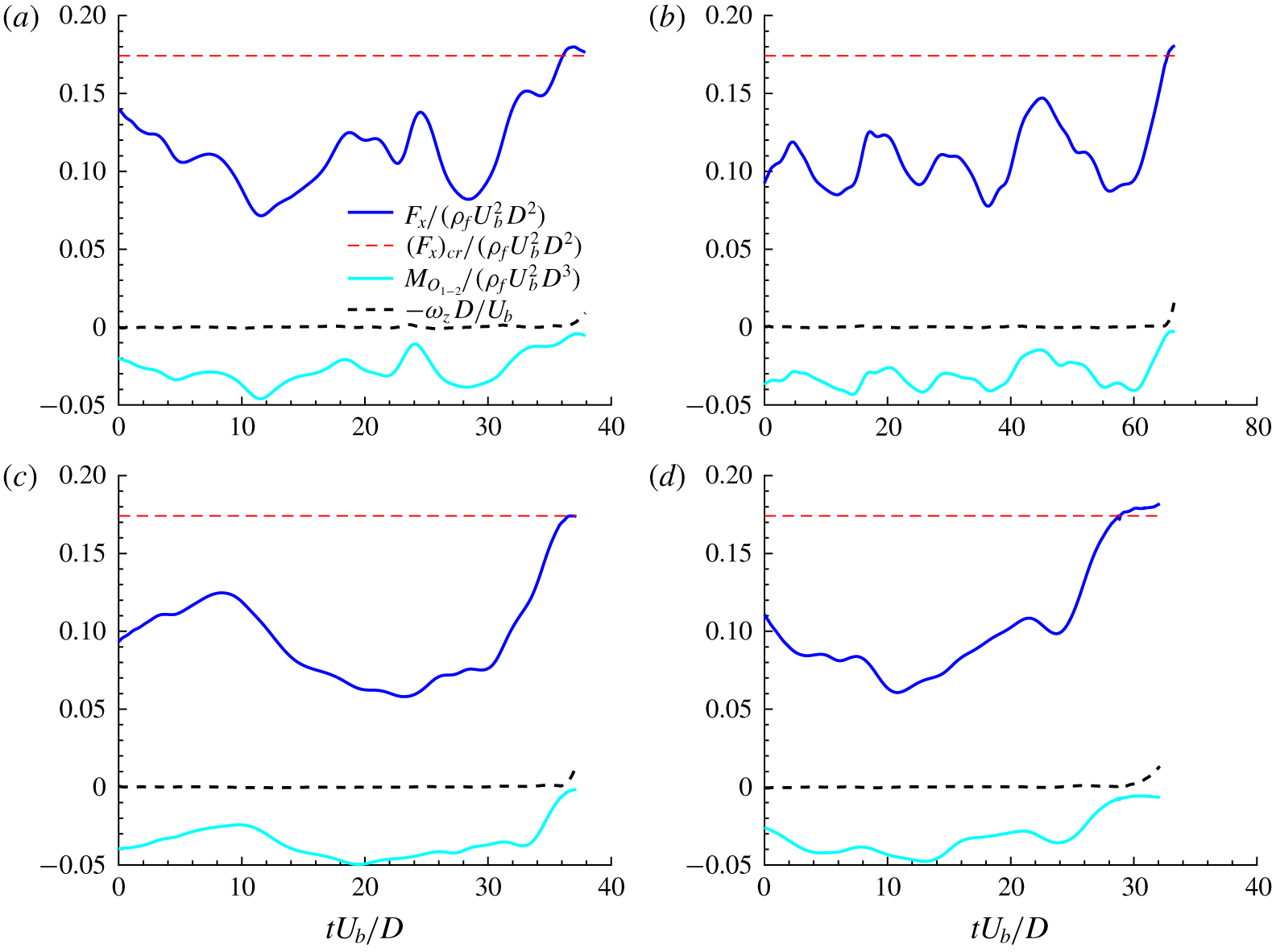
Figure 18. Time series of the streamwise fluid surface force exerted on the particle for four of the different instances of the incipient movement in the case  $Ga310$ (solid blue line). The dashed red line depicts the critical force value based on (3.2), the cyan line shows the total moment of the fluid-induced force and the particle submerged weight around $O_{1-2}$, and the dashed black line shows the spanwise angular velocity of the sediment particle.
To compare these two criteria, figure 18 shows the history of the streamwise fluid force, the total moment of all forces acting on the sediment particle and the spanwise angular velocity for four instances of incipient motion at  $Ga310$. As one can infer from the angular velocity, the time history is shown until the sediment particle starts to roll. The cyan solid line depicts the moment of the total fluid force (all components) together with that of the particle submerged weight at the contact points (around $O_{1-2}$). The data clearly show that the incipient motion occurs as soon as the torque of the fluid-induced surface force overcomes that of the particle submerged weight. The streamwise force history is compared to the corresponding critical value $F_{x,cr}$ obtained from (3.2). In all cases, once the critical force value is reached (i.e. the solid blue line crosses the dashed red line), the particle rolls, which is consistent with the force-based criterion. This confirms that considering only the streamwise component of the fluid-induced force suffices for predicting the onset of sediment motion. The fact that the streamwise component of the fluid-induced force is predominant for the dislodgement of highly exposed sediment particles can also be inferred from figure 14(b), because at the start of rolling the positive streamwise velocity fluctuation contributes much more to the Reynolds shear stress than the negative bed-normal component. From the present dataset, we could not observe any instance where the force-based criterion fails to predict dislodgement, while the impulse-based criterion succeeds. In other words, we did not observe a force larger than the critical value that could not dislodge the particle due to a too short duration. Yet, we should note that the sampling time in the present work is much smaller than that of the experiments of Celik et al. (Reference Celik, Diplas, Dancey and Valyrakis2010), due to the high costs of interface resolved simulations. Moreover, the ratio between the particle diameter and the smallest flow structures is approximately $20$ times larger in the high-Reynolds-number experimental study ( $D^{+}\approx 20$ in the present work, compared to ${\approx}400$ in the experimental study).

Figure 19. (a) Time series of the streamwise fluid surface force exerted on the particle for the test case with the particle diameter twice that of the main cases, i.e.  $D^{\prime }=2D$ (solid blue line). The dashed red line depicts the critical force value, and the shaded area the impulse during the period when $F_{x}>(F_{x})_{cr}$; the blue vertical line denotes the time for which the contours of the normal stress are plotted. (b) Contours of the normal stress plotted on the surface of a sphere with same centre as the sediment particle and radius $D^{\prime }/2+3\unicode[STIX]{x0394}x$, at the instant marked by the vertical line in panel (a). The perspective correspond to that of an observer aligned with the positive streamwise direction.
To confirm the hypothesis that a force-based criterion for sediment dislodgement may fail when a larger particle is considered, we have performed an auxiliary DNS with a particle with diameter  $D^{\prime }$ twice as large, while keeping the bulk Reynolds number and Shields parameter equal to those of case $Ga310$, i.e. a sediment particle with size of $D^{\prime +}\approx 40$ and Galileo number of $620$. Figure 19(a) shows a segment of the time history of the streamwise flow-induced force on the particle after its release, while the surface contours of the pressure for an instance with a streamwise fluid force greater than that of the critical value, are illustrated in the panel (b) of the same figure. We observe here and in several other instances that the force exceeds the critical value, but the particle remains stationary in its resting pocket. The shaded area in the figure represents the impulse, which the criterion in the study of Celik et al. (Reference Celik, Diplas, Dancey and Valyrakis2010) is based on. Indeed, when considering a larger particle we have found instances where, though the streamwise force is sufficiently high to promote dislodgement, the time scale at which it acts is not sufficiently long. Chan-Braun et al. (Reference Chan-Braun, García-Villalba and Uhlmann2011) and Mazzuoli & Uhlmann (Reference Mazzuoli and Uhlmann2017) among others showed that the interaction of small vortices with a relatively large sphere (i.e. for large values of $D^{+}$) results in fluctuations of the force acting on the particle due to the filtering of vortices smaller than the particle size. Therefore, the dynamics of the particles is mostly driven by vortices of length scale comparable with that of the particles, so larger particles and larger vortex sizes are associated with stronger forces and longer time scales. This is quantified in figure 20, where the spectra of the streamwise fluid surface force exerted on the particle normalised by the critical force value for the two different particle sizes considered ( $D^{+}=21.5$ in blue and $D^{+}=43$ in red) are compared. The vertical lines in the figure denote the angular frequency at each particle size. The data in the figure show that, for the bigger particle, the effect of the flow structures with a time scale comparable or larger than that of the bigger particle (angular frequencies smaller than the red vertical line) is larger than the effect of structures of similar time scale on the smaller particle, which confirms that the filter at the particle scale dissipates more energy in the case of smaller particles.

Figure 20. Spectra of the streamwise fluid surface force exerted on the particle for different particle size:  $D^{+}=21.5$ (blue) and $D^{+}=43$ (red), normalised by the critical force value for each size. The vertical lines denote the angular frequency at each particle size.
4 Conclusions
We have used interface-resolved simulations to study the dynamics of a sediment particle, initially at rest on a fixed porous bed, in a turbulent open channel flow. A relatively small particle (diameter  $D\approx 20\unicode[STIX]{x1D708}/u_{\unicode[STIX]{x1D70F}}$) is subjected to a turbulent flow, for different relative strengths of buoyancy to shear-induced boundary force, quantified by the Shields parameter. In practice, we have explicitly varied the Galileo number, since it can be computed a priori from the flow governing parameters.
We have shown that, for the cases with lower Galileo numbers (below  $150$), the sediment dislodgement is driven by the mean flow: the particle promptly lifts-off when exposed to the turbulent field, irrespective of the specific turbulent initial condition. Two classical modes of sediment transport, resuspension and saltation, have been reproduced by the simulations and analysed.
In the resuspension mode, the particle travels suspended in the flow with an oscillatory path. These oscillations are explained by the balance between the shear-induced lift force, which decreases when increasing the distance from the wall, and gravity. This regime is characterised by a flow-induced lift force of the same order of magnitude as the particle submerged weight ( $(\unicode[STIX]{x1D70C}_{p}-\unicode[STIX]{x1D70C})gV_{p}$) and the bed shear-induced force ( $\unicode[STIX]{x1D70C}u_{\unicode[STIX]{x1D70F}}^{2}A_{p}$), that the particle weight is mainly balanced by the lift force induced by the mean flow. Moreover, we show that although the bulk dynamics of the sediment particle is correlated with the apparent slip velocity and the local shear rate experienced by the particle, the effect of turbulent fluctuations and contact forces on the particle acceleration is not negligible.
The saltation mode, case  $Ga150$, is characterised by a high-frequency bouncing trajectory, with its vertical component resembling the bouncing motion of a sphere colliding onto a planar wall (Gondret et al. Reference Gondret, Lance and Petit2002). Here the acceleration is almost constant throughout most of the motion (approximately $0.5g$), except very close to the bed. Then, as the particle approaches the wall, it experiences short-range hydrodynamic interactions, and ultimately collisions which induce, expectedly, a very strong vertical acceleration. This positive acceleration is quenched by the gravitational force and by an increased drag until the particle starts falling again. In this case, the fluid surface force has the same order of magnitude as the particle submerged weight, but is almost $30$ times larger than the shear-induced boundary force. Despite this, whenever the sediment particle has a significant apparent slip velocity (with respect to the mean flow), the shear-induced lift force plays an important role on the sediment particle dynamics. This is the case when the streamwise velocity of the particle is reduced considerably due to a collision (see figure 9c), or in the beginning of the simulation, since the particle is at rest.
We have then considered cases where the flow governing parameters are such that the particle motion is dictated by extreme turbulent events. Two different values of the Galileo number,  $250$ and $310$, have been examined here. The main difference between the trajectories for the two cases is the resting times, and the probability of onset of motion. The Shields parameter is approximately $0.005$ for these cases – much smaller than the corresponding critical value. The flow events triggering the sediment motion are captured by sampling the flow field upstream of the particle, just prior to its movement. Consistently with previous experimental studies (see e.g. Nelson et al. (Reference Nelson, Shreve, McLean and Drake1995), Hofland (Reference Hofland2005), Dwivedi et al. (Reference Dwivedi, Melville and Shamseldin2010)), our results show that intense streamwise velocity fluctuations, associated with the sweeps, are the main cause of sediment motion. Visualisations of the flow structure at the moment of incipient motion showed that these events are associated with the tail of a hairpin-like vortex, travelling near the particle. Taking further advantage of the three-dimensional nature of the DNS data, we have investigated the pressure distribution close to the surface of the sediment particle at the moment of incipient motion. For all the instances detected, this distribution shows a consistent footprint of the passage of the hairpin vortex: an increased stagnation pressure zone upstream due to a higher than mean streamwise velocity fluctuation, and a high-pressure region close to the contact point of the particle with the bed.
Finally, previously proposed criteria for the onset of sediment transport, based on the concept of a critical impulse (Celik et al. Reference Celik, Diplas, Dancey and Valyrakis2010), have been tested against the numerical results for these cases at higher Galileo numbers. Our results clearly demonstrate that, for the present set-up, a critical threshold streamwise force effectively predicts the incipient motion. Although the principle behind the impulse-based criteria for predicting the onset of sediment transport seems more rigorous, in the present set-up a force exceeding the corresponding critical value was always able to move the sediment particle, regardless of its duration. This might be a consequence of the relatively low Reynolds number of the DNS, where extreme turbulent events with a typical time scale of  $D/u_{\unicode[STIX]{x1D70F}}$ always act on a long enough time to move the sediment particle. Indeed, a test simulation with a larger particle size at the same Reynolds number showed instances of the force exceeding the critical value, while the sediment particle remained stationary. Thus, simulations at higher Reynolds number and varying particle sizes could provide further insights on the necessary conditions for turbulence-induced impulses capable of dislodging relatively larger sediment particles.
Acknowledgements
This work was supported by the European Research Council grant no. ERC-2013- CoG-616186, TRITOS and by the Swedish Research Council grant no. VR 2014-5001. The authors acknowledge computer time provided by SNIC (Swedish National Infrastructure for Computing). The authors acknowledge the anonymous referees for useful comments on an earlier version of the manuscript.
Declaration of interests
The authors report no conflict of interest.


 Open access