


1. Introduction
Research on canopy flows originated from the study of flows interacting with natural organisms such as trees, grasses and coral reefs (Raupach & Thom Reference Raupach and Thom1981; Finnigan Reference Finnigan2000; Monismith Reference Monismith2007; de Langre Reference de Langre2008; Belcher, Harman & Finnigan Reference Belcher, Harman and Finnigan2012; Nepf Reference Nepf2012; Lowe & Falter Reference Lowe and Falter2015; Chen, Chamecki & Katul Reference Chen, Chamecki and Katul2019), and its scope has been expanded to many engineering and environmental applications, including wind farms (Calaf, Meneveau & Meyers Reference Calaf, Meneveau and Meyers2010; Stevens & Meneveau Reference Stevens and Meneveau2017; Ali et al. Reference Ali, Hamilton, Calaf and Cal2019) and urban atmospheres (Fernando Reference Fernando2010). A canopy flow features coherent turbulent structures that develops from the Kelvin–Helmholtz instability induced by the difference in velocity between the inside and outside the canopy owing to the canopy drag (Naudascher & Rockwell Reference Naudascher and Rockwell1994; Bailey & Stoll Reference Bailey and Stoll2016; Luminari, Airiau & Bottaro Reference Luminari, Airiau and Bottaro2016; Singh et al. Reference Singh, Bandi, Mahadevan and Mandre2016; Zampogna et al. Reference Zampogna, Pluvinage, Kourta and Bottaro2016; Monti, Omidyeganeh & Pinelli Reference Monti, Omidyeganeh and Pinelli2019; Monti et al. Reference Monti, Omidyeganeh, Eckhardt and Pinelli2020; Sharma & García-Mayoral Reference Sharma and García-Mayoral2020b; Chung & Koseff Reference Chung and Koseff2021). In flexible canopies, the coherent turbulent structures in the mixing layer interact with the canopy, thereby propagating the wavy deformation of the canopy, a phenomenon known as monami (Inoue Reference Inoue1955; Ghisalberti & Nepf Reference Ghisalberti and Nepf2002; Tschisgale, Meller & Frohlich Reference Tschisgale, Meller and Frohlich2017b; Tschisgale et al. Reference Tschisgale, Löhrer, Meller and Fröhlich2021; Mandel et al. Reference Mandel, Gakhar, Chung, Rosenzweig and Koseff2019; O'Connor & Revell Reference O'Connor and Revell2019; Wong, Trinh & Chapman Reference Wong, Trinh and Chapman2020; Houseago et al. Reference Houseago, Hong, Cheng, Best, Parsons and Chamorro2022), which influences both the transport of momentum into the canopy and the momentum mixing inside the canopy (Ackerman & Okubo Reference Ackerman and Okubo1993; Okamoto & Nezu Reference Okamoto and Nezu2009; Caroppi et al. Reference Caroppi, Västilä, Järvelä, Rowiński and Giugni2019, Reference Caroppi, Västilä, Gualtieri, Järvelä, Giugni and Rowiński2021).
Nevertheless, the energy flux within the canopy flow remains poorly understood. The presence of the canopy complicates the flow of energy because the spatial inhomogeneity caused by the stems inside the canopy and the correlation between the canopy drag and flow velocity lead to several new terms in the budget equation for the turbulent kinetic energy (TKE) and a dispersive component of the kinetic energy known as dispersive kinetic energy (DKE) (Finnigan Reference Finnigan2000). Although a few pioneering studies have attempted to investigate these terms (Finnigan Reference Finnigan1979; Raupach & Thom Reference Raupach and Thom1981; Dwyer, Patton & Shaw Reference Dwyer, Patton and Shaw1997; Finnigan Reference Finnigan2000; Poggi et al. Reference Poggi, Porporato, Ridolfi, Albertson and Katul2004; Yue et al. Reference Yue, Meneveau, Parlange, Zhu, Kang and Katz2008), the current understanding of the flow field and its underlying mechanisms is still insufficient. For example, owing to the difficulty of experimentally measuring the canopy drag–flow velocity correlation, the role of the waving term, which is associated with this correlation, remains unclear and thus has usually been neglected in previous modelling efforts (Finnigan Reference Finnigan1979; Raupach & Thom Reference Raupach and Thom1981; Finnigan Reference Finnigan2000). In addition, field and laboratory experiments have observed the direct flow of energy from large scales to small scales, also known as the ‘spectral shortcut’ (Allen Reference Allen1968; Seginer et al. Reference Seginer, Mulhearn, Bradley and Finnigan1976; Kaimal & Finnigan Reference Kaimal and Finnigan1994; Brunet, Finnigan & Raupach Reference Brunet, Finnigan and Raupach1994), which has been considered to develop turbulence models for canopy flow simulations (King, Tinoco & Cowen Reference King, Tinoco and Cowen2012). However, previous experiments measured only the frequency energy spectra and then derived the wavenumber energy spectra using Taylor's frozen hypothesis, whereas direct evidence derived from the spatial energy spectra is lacking. Furthermore, the detailed mechanism responsible for the spectral shortcut remains elusive.
The spectral analysis of the energy budget is a valuable tool for investigating turbulent energy processes, including the production, dissipation and transport of energy among different locations, across different scales and between different velocity components (Lumley Reference Lumley1964). Recently, such spectral analyses have been successfully employed in several channel flow studies. Cho, Hwang & Choi (Reference Cho, Hwang and Choi2018) studied the spanwise spectra of energy transfer for a friction Reynolds number  $Re_\tau = 1700$. They revealed two scale interaction processes (in addition to the normal energy cascade) in the near-wall region: one is the interaction between the energy-containing scales that generate skin friction, and the other interaction is the downward energy transfer from small to large scales related to the formation of wall-reaching motions containing inactive energy. Lee & Moser (Reference Lee and Moser2019) studied the streamwise and spanwise spectra of energy transfer for $Re_\tau = 5200$ and showed that TKE is produced in the streamwise velocity component at streamwise-elongated modes, transferred to the modes with higher spanwise wavenumbers, and redistributed to the vertical and spanwise velocity components by pressure intercomponent transport across a broad band of wavenumbers. They also found that the streamwise-elongated modes modulate the near-wall dynamics by wall-normal turbulent transport, which was also discovered by Mizuno (Reference Mizuno2016). Both Cho et al. (Reference Cho, Hwang and Choi2018) and Lee & Moser (Reference Lee and Moser2019) observed an inverse energy cascade where TKE flows from small to large scales, which was not detected in earlier studies by Domaradzki et al. (Reference Domaradzki, Liu, Härtel and Kleiser1994) and Bolotnov et al. (Reference Bolotnov, Lahey, Drew, Jansen and Oberai2010), who studied channel flows with $Re_\tau = 210$ and $180$, respectively. Wang et al. (Reference Wang, Zhang, Hao, Huang, Shen, Xu and Zhang2020) performed spectral energy budget analyses for turbulent winds over a flat surface, a slow water wave and a fast water wave, and found that waves contribute energy to the dominant wavelength scale close to the wave surface via the production term and enhance the spatial transport of turbulence towards the surface. For the cases with waves, an inverse energy cascade was observed to transport energy from small-scale motions to turbulent scales at the dominant wavelength scale close to the wave surface. In the present study, a spectral analysis of the energy budget of canopy flows is performed for the first time to understand the transfer of turbulent energy in canopies.
In recent years, substantial advancements in canopy flow simulations have been reported. The Reynolds-averaged Navier–Stokes equations were first simulated using the  $k$-
$k$- $\epsilon$, $k$-
$k$- $\omega$ and Spalart–Allmaras turbulence models (López & García Reference López and García1998, Reference López and García2001; Li & Yan Reference Li and Yan2007; King et al. Reference King, Tinoco and Cowen2012), all of which require a priori parameter values for the simulation cases. With the increase in computational capabilities in recent years, the large-eddy simulation (LES) technique, which is computationally more expensive but requires less modelling effort, has become quite popular. Li & Xie (Reference Li and Xie2011) simulated a free-surface flow over a flexible canopy using a very large eddy simulation (LES) where the filter size in the Smagorinsky model was one-tenth of the water depth. More recently, Yan et al. (Reference Yan, Nepf, Huang and Cui2017) studied the flow and mass transfer in an open-channel canopy flow by applying the dynamic Smagorinsky model and introducing an additional diffusivity to model the effect of stem wakes.
Most previous simulations modelled the canopy as a continuous medium for which the drag coefficient needed to be prescribed. However, the assumption of a constant drag coefficient has a poor performance for deformable canopies, and the existing drag coefficient prediction models are complex and have achieved only limited success for specific cases (Okamoto & Nezu Reference Okamoto and Nezu2010; Pan, Chamecki & Isard Reference Pan, Chamecki and Isard2014a). Therefore, new simulation approaches that explicitly resolve the flow–canopy interaction are desirable. For instance, the immersed boundary (IB) method solves fluid–structure interactions on fixed Cartesian grids, making it a powerful tool for problems with complex structural geometries and kinematics (Peskin Reference Peskin1972; Kim et al. Reference Kim, Zhu, Wang and Peskin2003; Mittal & Iaccarino Reference Mittal and Iaccarino2005; Sotiropoulos & Yang Reference Sotiropoulos and Yang2014; Tschisgale, Kempe & Fröhlich Reference Tschisgale, Kempe and Fröhlich2017a; Calderer et al. Reference Calderer, Guo, Shen and Sotiropoulos2018; Kim & Choi Reference Kim and Choi2019; Huang & Tian Reference Huang and Tian2019; Monti et al. Reference Monti, Omidyeganeh, Eckhardt and Pinelli2020; Sharma & García-Mayoral Reference Sharma and García-Mayoral2020a; He et al. Reference He, Yang, Sotiropoulos and Shen2022; Zeng, Bhalla & Shen Reference Zeng, Bhalla and Shen2022). Hence, by resolving the stems in the canopy with the IB method, the drag on the stems can be obtained directly; i.e. no a priori drag coefficient is required. Moreover, the details of the correlation between the drag force and flow velocity can be obtained to analyse the waving term in the energy budget.
In this study, we simulate turbulent aquatic canopy flows with LES and resolve the stems in the canopy with an IB method. The simulation cases cover a broad range of stem flexibilities from rigid stems to oscillatory stems to stems yielding to the flow. Consequently, monami is also resolved. Conditional averaging with respect to the stem kinematics is performed to quantify the correlation between the flow features and monami wave phase. In addition, the spectral TKE budget is analysed for the first time to comprehensively understand the energy fluxes in canopies. In particular, the role of the waving term in the energy transfer in the canopy is resolved, and the canopy drag–flow velocity correlation is studied to understand the mechanism responsible for the waving term. Furthermore, a triadic analysis is conducted to investigate the energy transfer among different scales.
The remainder of this paper is organized as follows. The numerical algorithms employed for the LES and the parameters of the computational cases are described in § 2. An overview of the flow field, including the instantaneous flow velocity and canopy kinematics, the vertical profiles of the flow statistics, the monami statistics and the conditional averages of the flow velocity and canopy drag, is described in § 3. Spectral analyses of the TKE and DKE budgets are presented in § 4. Finally, the conclusions are given in § 5.
2. Simulation methods
2.1. Flow simulation
In this study, we consider a three-dimensional (3-D) turbulent flow over a periodic array of flexible canopy stems, as shown in figure 1. Details of the dimensions of the computational cases are given in § 2.5. Here, we focus on the mathematical formulation and numerical method. In the Cartesian coordinate system,  $x_i(i=1,2,3) = (x,y,z)$, $x$,
$x$,  $y$ and $z$ indicate the streamwise, vertical and spanwise directions, respectively. The resolved velocity components in the LES are denoted by $u_i(i=1,2,3) = (u,v,w)$, which are governed by the following continuity and momentum equations:
 \begin{gather} \frac{\partial u_i}{\partial x_i} = 0, \end{gather}
 \begin{gather}\frac{\partial u_i}{\partial t}+ \frac{\partial u_i u_j}{\partial x_j} = \dfrac{1}{\rho_f}\left(-\frac{\partial p}{\partial x_i} + \mu\frac{\partial {\mathsf{S}}_{ij}}{\partial x_j} + \rho_f g_i - \frac{\partial \tau_{sgs,ij}}{\partial x_j} \right) + f_i, \end{gather}
where  $t$ denotes time, $\rho _f$ is the volumetric fluid density, $p$ is the resolved modified pressure in the LES, $\mu$ is the dynamic viscosity of the fluid, ${\mathsf{S}}_{ij} = ({\partial u_i}/{\partial x_j} + {\partial u_j}/{\partial x_i})/2$ is the resolved strain rate tensor, $g_i$ is the gravitational acceleration constant, $f_i$ is the resolved drag force exerted by the canopy and $\tau _{sgs,ij}$ is the subgrid-scale (SGS) stress, which is modelled by the dynamic Smagorinsky model (Smagorinsky Reference Smagorinsky1963; Germano et al. Reference Germano, Piomelli, Moin and Cabot1991; Lilly Reference Lilly1992).

Figure 1. Configuration of the simulation set-up. The flow is driven by a pressure gradient along the streamwise direction over an evenly spaced  $40\times 5$ array of stems. Here $h$ stands for the height of an undeformed stem.
Our flow simulation is performed on a staggered Cartesian grid (Harlow & Welch Reference Harlow and Welch1965). Equation (2.1b) is spatially discretized by a second-order central difference scheme and temporally integrated by the second-order Runge–Kutta (RK2) method. During each substep of the RK2 method, the fractional-step approach (Kim & Moin Reference Kim and Moin1985) is employed to enforce the continuity equation (2.1a), where the pressure is solved by a Poisson equation,
 \begin{equation} \frac{\partial}{\partial x_i} \left(\frac{1}{\rho_f}\frac{\partial p}{\partial x_i}\right) = \frac{1}{\alpha \Delta t}\frac{\partial u_i^*}{\partial x_i}, \end{equation}
where  $\alpha$ is 1.0 and 0.5 in the first and second substeps of RK2, respectively; $\Delta t$ is the time step of the simulation; and $u_i^*$ is calculated by
 \begin{equation} u_i^* = u_i + \Delta t\left[\dfrac{1}{\rho_f}\left(\mu\frac{\partial {\mathsf{S}}_{ij}}{\partial x_j} + \rho_f g_i - \frac{\partial \tau_{sgs,ij}}{\partial x_j} \right) + f_i - \frac{\partial u_i u_j}{\partial x_j}\right]. \end{equation}
Equation (2.2) is solved by the Portable, Extensible Toolkit for Scientific Computation math library (Abhyankar et al. Reference Abhyankar, Brown, Constantinescu, Ghosh, Smith and Zhang2018). The details of the numerical schemes of our code, its applications to various flows and validations can be found in Liu (Reference Liu2013), Xie et al. (Reference Xie, Yang, Liu and Shen2016), Yang et al. (Reference Yang, Lu, Guo, Liu and Shen2017), Yang et al. (Reference Yang, He, Ouyang, Anderson, Shen and Hogan2018a) and Liu et al. (Reference Liu, He, Shen and Hong2021).
2.2. Stem simulation
The stems are modelled following Huang, Shin & Sung (Reference Huang, Shin and Sung2007) as inextensible nonlinear Euler–Bernoulli beams. The governing equation for the deformation of each stem is
 \begin{equation} \rho_d \dfrac{\partial^2 X_i}{\partial t^2} = \dfrac{\partial}{\partial s}\left(T \frac{\partial X_i}{\partial s}\right) - \dfrac{\partial^2}{\partial s^2}\left(\gamma \dfrac{\partial^2 X_i}{\partial s^2}\right) + \rho_d g_i + F_i, \end{equation}
where  $s$ is the local coordinate along the stem, $X_i = X_i(s,t)$ is the displacement of the stem in the $i$ direction, $T$ is the tension coefficient, $\gamma$ is the bending rigidity, $F_i$ is the hydrodynamic force on the stem and $\rho _d = \rho _s - \rho _f$, where $\rho _s$ is the volumetric density of the stem. For a stem whose cross-section is rectangular, $\gamma = Ed^2/12$, where $E$ is Young's modulus and $d$ is the stem thickness. Note that the density is the linear density in the original equations in Huang et al. (Reference Huang, Shin and Sung2007). But in (2.4), the density is the volumetric density. Therefore, $\gamma = EI = Ebd^3/12$ in Huang et al. (Reference Huang, Shin and Sung2007), where $b$ denotes the stem width, should be divided by the cross-section area $bd$ to obtain $\gamma$ in (2.4). The first three terms on the right-hand side are successively the tension force, the bending force and the summation of the gravity and buoyancy forces. Also, note that the density in the left-hand side term is $\rho _d$ instead of $\rho _s$, because the stem thickness is too small to be resolved in the flow simulation. As a result, the buoyancy force is included in the third right-hand side term instead of being resolved in the hydrodynamic force on the stem. Detailed derivation can be found in the appendix of Huang & Sung (Reference Huang and Sung2009). We further assume that the stem is inextensible such that
 \begin{equation} \frac{\partial X_k}{\partial s}\frac{\partial X_k}{\partial s} = 1. \end{equation}
 To solve the above equations, we first obtain the tension coefficient  $T$ from the Poisson equation derived from (2.4) and (2.5),
 \begin{equation} \frac{\partial X_k}{\partial s}\dfrac{\partial^2}{\partial s^2}\left(T\frac{\partial X_k}{\partial s}\right) = \dfrac{1}{2}\dfrac{\partial^2}{\partial t^2}\left(\frac{\partial X_k}{\partial s}\frac{\partial X_k}{\partial s}\right)-\dfrac{\partial^2 X_k}{\partial t \partial s}\dfrac{\partial^2 X_k}{\partial t \partial s}-\frac{\partial X_k}{\partial s}\frac{\partial}{\partial s}\left(F_{b,k} + F_k\right), \end{equation}
where  $F_{b,k} = -({\partial ^2}/{\partial s^2})(\gamma ({\partial ^2 X_k}/{\partial s^2}))$ is the bending force. Then, the tension coefficient is substituted into (2.4) to solve for $X_i$. The stem is modelled with a free end and a clamped end. The boundary conditions for the free end are
 \begin{equation} T = 0,\ \dfrac{\partial^2 X_i}{\partial s^2}=0,\ \dfrac{\partial^3 X_i}{\partial s^3}=0, \end{equation}
and the boundary conditions for the clamped end are
 \begin{equation} X_i = X_{0,i},\ \frac{\partial X_i}{\partial s} = \frac{\partial X_{0,i}}{\partial s}, \end{equation}
where  $X_{0,i}(s)=X_i(s,t=0)$ is the initial condition. Details of the numerical algorithms employed for the stem simulation can be found in Huang et al. (Reference Huang, Shin and Sung2007).
In this study, we use a nonlinear Euler–Bernoulli beam model, which is based on the assumptions that a cross-section remains plane after deformation, and the neutral axis keeps perpendicular to the cross-section during deformation. As a result, the effects of transverse shear deformation and rotational bending are omitted (Bauchau & Craig Reference Bauchau and Craig2009). This treatment requires that the structure thickness is much smaller than the length and width, which is the case in this study. The beams in this study can only bend in the streamwise–vertical plane (see the discussions in § 2.5). We note that the canopy flow simulation by Tschisgale & Fröhlich (Reference Tschisgale and Fröhlich2020) used a Cosserat rod model, where the rod elements can have both translational and rotational degrees of freedom to allow rod twisting. For thick beams where the transverse shear deformation and rotational bending need to be considered, the Timoshenko–Ehrenfest beam theory can be applied (Hutchinson Reference Hutchinson2001). For structures undergoing significant two-dimensional (2-D) deformation, a shell model should be applied, such as the Kirchhoff–Love thin shell theory (Elishakoff Reference Elishakoff2020), which is a 2-D extension of the Euler–Bernoulli beam model and is often applied to thin shells. It is based on the assumption that the straight lines initially normal to the midsurface keep straight and perpendicular to the midsurface after deformation. Another shell model is the Uflyand–Mindlin plate theory, which is often employed when the plate is thick enough to have prominent shear deformation along the shell thickness (Elishakoff Reference Elishakoff2020).
2.3. Coupling fluid and stem dynamics by an IB method
The one-dimensional (1-D) filaments in the streamwise–vertical plane introduced in § 2.2 are expanded in the spanwise direction to form the 2-D stems with finite width. The dynamics of the fluid and canopy stems are coupled through the force terms, namely,  $f_i$ in (2.1b) and $F_i$ in (2.4), by an IB method (Mittal & Iaccarino Reference Mittal and Iaccarino2005). As the original Lagrangian grid on the filaments is 1-D and is relatively coarser than the background Eulerian grid, we use an additional 2-D structural Lagrangian grid, which is uniformly distributed on the stem surface and has the same resolution as the background Eulerian grid, to obtain the coupling between the stems and flow.
We use the penalization approach developed by Goldstein, Handler & Sirovich (Reference Goldstein, Handler and Sirovich1993), where the hydrodynamic force on the 2-D Lagrangian grid on the structure,  $F_{2D,i}(s_1,s_2,t)$, is calculated by
 \begin{align} F_{2D,i}(s_1,s_2,t)&=\alpha \int_0^t\left[U_{f,i}(s_1,s_2,\tau)-U_i(s_1,s_2,\tau)\right]\,\mathrm{d}\tau\nonumber\\ &\quad + \beta \left[U_{f,i}(s_1,s_2,t)-U_i(s_1,s_2,t)\right], \end{align}
where  $(s_1,s_2)$ is the coordinate of the 2-D structural Lagrangian grid nodes, $U_{f,i}$ is the interpolated fluid velocity on the structure, $U_i={\rm d}X_i/{\rm d}t$ is the Lagrangian velocity of the structure, and $\alpha$ and $\beta$ are two parameters with dimensions of $ML^{-3}T^{-2}$ and $ML^{-3}T^{-1}$, respectively, for numerical simulation purposes. Suppose that $F_i$ is the only hydrodynamic force on the structure, $F_i = \rho _f \,{\rm d}(U_{f,i}-U_i)/{\rm d}t$; then, (2.9) describes the behaviour of a mass–spring–damper system about the relative velocity between the flow and the structure, $U_{f,i}-U_i$, as
 \begin{equation} \rho_f \frac{\mathrm{d}\left(U_{f,i}-U_i\right)}{\mathrm{d}t}- \beta \left(U_{f,i}-U_i\right) - \alpha \int_0^t\left(U_{f,i}-U_i\right)\,\mathrm{d}t^\prime = 0. \end{equation}
The natural frequency  $\omega _n$ and the damping ratio of this system $\zeta$ are expressed as
 \begin{equation} \omega_n = \sqrt{\frac{-\alpha}{\rho_f}}, \quad \zeta={-}\frac{\beta}{2\sqrt{-\alpha\rho_f}}. \end{equation}
Therefore, as the parameters of this system,  $\alpha$ and $\beta$ have physical significance in controlling its response behaviour. The frequencies of the energetic flow structures must be lower than $\omega _n$ to be resolved, which requires a large value of $-\alpha$. However, if the $-\alpha$ value is too large, numerical instability arises (Goldstein et al. Reference Goldstein, Handler and Sirovich1993). A moderate $\alpha$ value should therefore be selected to balance the numerical stability and the resolution of the energetic flow structures. Additionally, a large $-\beta$ value can strengthen the numerical stability, but to avoid overdamping, $-\beta$ should not be too large (Goldstein et al. Reference Goldstein, Handler and Sirovich1993). While $\alpha$ and $\beta$ have physical significance, usually they are still obtained by tuning and testing (e.g. Huang et al. Reference Huang, Shin and Sung2007, figure 13). Details on the selection and testing of the $\alpha$ and $\beta$ values in our simulations are given in § 2.5.
After  $F_{2D,i}(s_1,s_2,t)$ is obtained, it is averaged in the spanwise direction and then assigned to the nearest 1-D Lagrangian grid node on the stem to obtain $F_i(s,t)$, which is then used in (2.4) to update the stem deformation.
The interpolated fluid velocity on the stem,  $U_{f,i}$, is calculated by integrating the surrounding fluid velocity weighted by a Dirac delta function,
 \begin{equation} U_{f,i}(s_1,s_2,t) = \int_\varOmega u_i(x_1,x_2,x_3,t)\prod_{j=1}^3 \delta_j\left(X_j(s_1,s_2,t)-x_j\right)\,\mathrm{d} x_1 \,\mathrm{d} x_2 \,\mathrm{d} x_3, \end{equation}
where  $\varOmega$ indicates the computational domain and the Dirac delta function $\delta _j$ is defined as
 \begin{equation} \delta_j(r) = \frac{1}{\Delta x_j} \phi\left(\frac{r}{\Delta x_j}\right),\quad \text{no Einstein's summation notation on } j, \end{equation}
where the function  $\phi$ is (Peskin Reference Peskin2002)
 \begin{equation} \phi(r) = \begin{cases} \dfrac{1}{8}\left(3-2|r|+\sqrt{1+4|r|-4r^2}\right), & 0\leq|r|<1 \\[6 pt] \dfrac{1}{8}\left(5-2|r|-\sqrt{-7+12|r|-4r^2}\right), & 1\leq|r|<2\\ 0, & |r|\geq 2. \end{cases} \end{equation}
The delta function is also used to spread the Lagrangian hydrodynamic force on the structure,  $F_{2D,i}(s_1,s_2,t)$, to the Eulerian force on the background flow, $f_i(x_1,x_2,x_3,t)$,
 \begin{equation} f_i(x_1,x_2,x_3,t) ={-}\dfrac{d}{\rho_f}\int_\varGamma F_{2D,i}(s_1,s_2,t)\prod_{j=1}^3\delta_j\left(x_j-X_j(s_1,s_2,t)\right)\,\mathrm{d}s_1 \,\mathrm{d}s_2, \end{equation}
where  $\varGamma$ indicates all the stems. Note that in this algorithm, the fluid grid needs to be evenly spaced around the stem to conserve momentum (Yang et al. Reference Yang, Zhang, Li and He2009).
In summary, the coupling process between the flow and the stems for every time step is as follows.
(i) Expand the 1-D stem model (2.4) in the spanwise direction to form the 2-D stems.
(ii) Generate the 2-D structural Lagrangian grid on the stems.
(iii) Calculate the hydrodynamic force on the 2-D grid $F_{2D}(s_1,s_2,t)$ using (2.9).
(iv) Average
$F_{2D}(s_1,s_2,t)$ to calculate the force on the 1-D Lagrangian grid on the stems $F(s,t)$.(v) Update the deformation of the stems using (2.4).


2.4. Algorithm validation
We have performed extensive tests on these algorithms. The flow solver has been used in previous studies of various problems (Cui et al. Reference Cui, Yang, Jiang, Huang and Shen2017; Yang et al. Reference Yang, Lu, Guo, Liu and Shen2017; Yang, Deng & Shen Reference Yang, Deng and Shen2018b; Kan et al. Reference Kan, Yang, Lyu, Zheng and Shen2021; He Reference He2022). For the flow–stem interaction problem considered herein, three representative test cases are presented below. The first case is the flapping of a filament in a uniform flow following the numerical simulation in § 4.2 of Huang et al. (Reference Huang, Shin and Sung2007). In the test case, the Reynolds number is  $Re = \rho _f U_0 L/\mu = 200$, where $\rho _f, U_0, L$ and $\mu$ are the fluid density, incoming flow speed, filament length and fluid dynamic viscosity, respectively. Bending rigidity is $\gamma = 0$, dimensionless gravity along the streamwise direction is $g/(U_0^2/L) = 0.5$ and density $\rho _d d/\rho _f L = 1.5$, where $d$ is the filament thickness. Note that we exclusively use volumetric density while Huang et al. (Reference Huang, Shin and Sung2007) used linear density for the filament density, which causes different ways of normalization for the density. The computational domain size is $[0,8L]\times [0,8L]$, and the grid number is 512 and 250 along the streamwise ( $x$) and vertical directions ( $y$), respectively. The grid is uniformly distributed in the streamwise direction, and clustered in the vertical direction for $y\in [3L,5L]$ with a grid resolution of $\Delta y = 0.015625L$. The Dirichlet boundary condition with $u = U_0$ and $v = 0$ is applied at the inflow and far-field boundaries, and the convective boundary condition is applied at the outflow. There are 64 Lagrangian nodes along the filament. The filament is hinged at the upstream end. Initially, the filament is straight with an inclination of $0.1{\rm \pi}$ relative to the streamwise direction. We select $\alpha = -10^6, \beta = -10^3$ and $\Delta t = 0.0002.$ Our result for the steady oscillation amplitude and period of the filament is compared with Huang et al. (Reference Huang, Shin and Sung2007) and Zhu, He & Zhang (Reference Zhu, He and Zhang2014) in table 1. It is shown that our result agrees with the previous studies.
Table 1. Present simulation results for the flapping of a filament in a uniform flow compared with Huang et al. (Reference Huang, Shin and Sung2007) and Zhu et al. (Reference Zhu, He and Zhang2014).

The second case is the deformation of a flexible stem in a uniform water current following the experiment of Luhar & Nepf (Reference Luhar and Nepf2011), where the stem is clamped on the bottom wall. The Young's modulus of the stem is  $E = 500$ kPa, the stem length $h$ is 0.05 m, the stem width $b$ is 0.01 m and the stem thickness $d$ is $1.9 \times 10^{-3}$ m. The current velocity $U$ varies from $0.036\,{\rm m}\,{\rm s}^{-1}$ to $0.32\,{\rm m}\,{\rm s}^{-1}$. In our simulation, the domain size is $(1.0\,\text {m}, 0.3\,\text {m}, 0.1\,\text {m})$ in the streamwise, vertical and spanwise directions. Inlet and outlet boundary conditions are applied on the two boundaries in the streamwise direction, respectively, and a free-slip boundary condition is applied on the other boundaries. The plate is placed 0.2 m from the inlet and at the centre of the spanwise direction. The coordinate origin is located at the centre of the clamp line at the base of the stem. The $x$,
$x$,  $y$ and $z$ axes point to the downstream, upward and spanwise directions, respectively. The grid is refined within $([-0.05\,\text {m}, 0.2\,\text {m}], [0\,\text {m}, 0.1\,\text {m}], [-0.025\,\text {m}, 0.025\,\text {m}])$ with a grid resolution of $h/40$. The total grid number is $384\times 120\times 60$. Figure 2 plots the horizontal drag force on the stem as a function of the current velocity. Our result compares well with the measurement data of Luhar & Nepf (Reference Luhar and Nepf2011).

Figure 2. Comparison of the horizontal hydrodynamic drag  $F_x$ on the stem as a function of the inflow water current speed $U$ in the first validation case of § 2.4: $\square$, the result from the experiment by Luhar & Nepf (Reference Luhar and Nepf2011); $\vartriangle$, the result from the present simulation.
The third test case concerns a rigid canopy flow following the experimental study of Nezu & Sanjou (Reference Nezu and Sanjou2008). This case was also used as a validation case by Tschisgale & Fröhlich (Reference Tschisgale and Fröhlich2020) and Tschisgale et al. (Reference Tschisgale, Löhrer, Meller and Fröhlich2021). A  $10 \times 3$ array of rigid stems is placed on the bottom, and the computational domain size is $(3.2h, 3h, 1.92h)$ in the streamwise, vertical and spanwise directions. The length $h$, width $b$ and thickness $d$ of each stem are 0.05 m, 0.008 m and 0.001 m, respectively. The flow has a friction velocity at the bottom of $u^*= 0.0253\,{\rm m}\,{\rm s}^{-1}$. The same as the first test case, the grid resolution is $h/40$ for all three dimensions. Figure 3 compares our vertical profiles of the mean streamwise velocity and the Reynolds shear stress with the measurements of Nezu & Sanjou (Reference Nezu and Sanjou2008). Both curves agree with the experimental results.

Figure 3. Comparison of the horizontally averaged (a) mean streamwise velocity  $\langle \bar {u} \rangle$ normalized by the channel mean streamwise flow velocity $U_m$ and (b) Reynolds shear stress $-\langle \overline {u^\prime v^\prime }\rangle$ normalized by ${u^*}^2$ as functions of the vertical height $y$ normalized by the canopy height $h$ in the second validation case of § 2.4: $\square$, the result from the experiment by Nezu & Sanjou (Reference Nezu and Sanjou2008); ——, the result from the present simulation.
2.5. Parameters of simulation cases
The simulation set-up is visualized in figure 1. The physical parameters and corresponding dimensionless numbers are given in table 2. The channel dimensions are  $(L_x, H, L_z) = (20h, 3h, 2.5h)$ in the streamwise ( $x$), spanwise ( $y$) and vertical ( $z$) directions, where $h$ is the height of the undeformed stem. Therefore, the submergence ratio $H/h$ is 3, which can be categorized as shallow submergence ( $H/h < 5$) where most submerged aquatic canopies are found (Nepf Reference Nepf2012). An array of aligned stems clamped on the bottom of an open channel is considered. The array has five rows parallel to the streamwise direction, and each row has $N_x = 40$ stems. The stem density $\rho _s$ is 1.5 times the fluid density $\rho _f$, which is within the range of the relative density of polyvinyl chloride to water and close to the set-up of previous studies, such as Tschisgale et al. (Reference Tschisgale, Meller and Frohlich2017b) where $\rho _s/\rho _f = 1.4$ was used. The stem width $b$ is $0.25h$. A similar set-up was adopted by Nezu & Sanjou (Reference Nezu and Sanjou2008) in their case A-10. The roughness density is defined as $\lambda _f = bh_c/S_s$, where $h_c$ is the canopy height and $S_s$ is the floor area occupied by each stem (Wooding, Bradley & Marshall Reference Wooding, Bradley and Marshall1973; Nepf Reference Nepf2012). The canopy height is different for each $Ca$ and must be obtained a posteriori; see § 3.3 for the statistics of and discussions on the different definitions of the canopy height. Here, the hydrodynamic canopy height is used, and the result for each case is shown in table 2. One can see that the canopy is dense, i.e. the value of $\lambda _f$ is high, for low-flexibility canopy and becomes transitional as $Ca$ increases, according to the definitions by Nepf (Reference Nepf2012). The buoyancy number $B=\rho _d bdg h^3/EI$ is 0 for all the cases (Pan et al. Reference Pan, Follett, Chamecki and Nepf2014b; Tschisgale et al. Reference Tschisgale, Löhrer, Meller and Fröhlich2021). The bottom and top boundary conditions of the open channel are no-slip and free-slip, respectively, and the boundary conditions in the streamwise and spanwise directions are periodic. The flow is driven by a constant pressure gradient ${\mathrm {d}p}/{\mathrm {d} x}$. The friction velocity $u^*$ satisfies $u^* = \sqrt {({1}/{\rho _f})({\mathrm {d}p}/{\mathrm {d} x})(H-h)}$. The Reynolds number defined by the canopy height and friction velocity is $Re_\tau = {u^* h}/{\nu } = 1000$. The grid resolution $\varDelta$ is $h/40$ for all three dimensions such that grid number is $800 \times 240 \times 100$. Note that the submergence ratio, the Reynolds number and the grid resolution in our simulation set-up are the same as, or close to, those in Nezu & Sanjou (Reference Nezu and Sanjou2008), whose set-up we use to validate our algorithm in § 2.4. However, our simulation cases account for stem flexibility, which substantially increases the computational cost.
Table 2. Physical parameters and dimensionless numbers in the present simulation.

The stem flexibility is quantified by the dimensionless Cauchy number  $Ca$, which denotes the ratio between the hydrodynamic force on the stem and the stem restoring force (Luhar & Nepf Reference Luhar and Nepf2016; Jin et al. Reference Jin, Kim, Hong and Chamorro2018a,Reference Jin, Kim, Mao and Chamorrob),
 \begin{equation} Ca = \dfrac{\rho_f u^{*2}bh^3}{EI}, \end{equation}
where  $I={bd^3}/{12}$ is the second moment of area of the stem cross-section. In our simulation cases, we consider $Ca = 0, 5, 30$ and $80$, where $Ca = 0$ corresponds to rigid stems and increasingly larger values of $Ca$ signify stems with greater flexibility. We notice that in Pan et al. (Reference Pan, Follett, Chamecki and Nepf2014b), the Cauchy number is defined as $Ca = \rho C_D bU^2 l^3/2EI$, where $C_D$ is the drag coefficient, $l$ is the filament length and $U$ is the characteristic velocity scale, which is selected as the mean bulk velocity $\bar {u}$ in this study. The present definition is similar to their definition, except that $C_D$ is not treated as an a priori drag coefficient, and the characteristic velocity is $u^*$ instead of $\bar {u}$ because $u^*$ is closely correlated with the canopy drag. Therefore, we keep the physical significance of $Ca$ that it represents the ratio between the stem drag and restoring force, while adapting the mathematical expression for $Ca$ such that it fits better the present simulation set-up. Regarding the choice of the Cauchy number, our stem flexibility covers a broad range from rigid stems ( $Ca = 0$) to oscillatory stems ( $Ca = 5$) to stems yielding to the flow ( $Ca = 30$ and 80) for the study of different monami scenarios.
We restrain the stem kinematics to the streamwise–vertical plane and neglect motions such as twisting that cause spanwise displacement. This simplification is based on the following considerations. First, the flow features, such as the coherent vortices in the mixing layer and the classification of different zones in the flow, are dominant in the vertical and streamwise directions, and these features interact with the stem kinematics in these two directions. Second, the streamwise–vertical displacement model for this array of stems is simpler and computationally more affordable than a general 3-D displacement model. We notice that the simulation by Fröhlich's group resolved the spanwise motion of the stem with a Cosserat rod model, but their visualizations of the instantaneous stem deformation did not show prominent spanwise deformation (e.g. Tschisgale et al. Reference Tschisgale, Kempe and Fröhlich2017a, figure 6; Tschisgale & Fröhlich Reference Tschisgale and Fröhlich2020, figure 21; Tschisgale et al. Reference Tschisgale, Löhrer, Meller and Fröhlich2021, figures 16 and 17). Considering that the stems in our simulation are wider than their stems, the stems in the present study are more rigid in the spanwise direction and are even less prone to spanwise motion. Therefore, we believe that limiting the stem motion in streamwise–vertical planes is an acceptable approximation with reduced computational cost.
For the values of  $\alpha$ and $\beta$ in (2.9), we select $\alpha /[\rho _f(u^*/h)^2] = -10^5$ and $\beta /[\rho _f u^*/h] = -10^2$, respectively, leading to $\omega _n = 316.2u^*/h$ and $\zeta = 0.158$ according to (2.11). This selection ensures that the dominant energetic flow structures are captured and that a reasonably large time step can be adopted without triggering numerical instability. To compare different values of $\alpha$ and $\beta$, we analysed a series of test cases involving two aligned stems with $Ca = 30$ and the same shape and interval distance as described above. We tested $\alpha /[\rho _f(u^*/h)^2]$ ranging from $-10^3$ to $-10^{5.5}$ and $\beta [\rho _f(u^*/h)]$ ranging from $-10^0$ to $-10^{2.5}$. Higher absolute values of $\alpha$ and $\beta$ were not considered because the time step would be excessively small. The resulting mean streamwise displacements at the tips of the upstream stem, $d_u$, and the downstream stem, $d_d$, are listed in table 3. The results are insensitive to $\alpha$ and $\beta$ when their magnitudes are large. Between $(\alpha /[\rho _f(u^*/h)^2] = -10^4, \beta /[\rho _f u^*/h] = -10^1)$ and $(\alpha /[\rho _f(u^*/h)^2] = -10^{5.5}, \beta /[\rho _f u^*/h] = -10^{2.5})$, the relative differences in $d_u$ and $d_d$ are small, both within 2 %. Hence, in our simulation cases presented below, $\alpha /[\rho _f(u^*/h)^2] = -10^5$ and $\beta /[\rho _f u^*/h] = -10^2$ are used.
Table 3. Mean streamwise tip displacements of two tandem stems normalized by the stem length ( $d_u/h, d_d/h$) for a range of $\alpha$ and $\beta$ values. The stems have $Ca = 30$, and their interval follows the simulation set-up described in § 2.5.

For every case, the characteristic wavenumber of monami,  $k_x h$, is no less than 0.63, which corresponds to wavelength $\lambda < 10.0h$. Therefore, the present streamwise domain size of $20h$ can ensure that at least two complete monami waves are captured. To test the present grid resolution and spanwise domain size, we performed a grid convergence test and a spanwise domain size independence test for the case $Ca = 5$. In the grid convergence test, we tested the grid sizes of $512 \times 160 \times 64$ and $1200 \times 360 \times 150$ and compared the vertical profiles of streamwise velocity $\langle \bar {u}\rangle /u^*$ and Reynolds shear stress $-\langle \overline {u^\prime v^\prime }\rangle /u^{*2}$ with the present grid size $800 \times 240 \times 100$ in figure 4(a,b). It shows that all the cases have similar profiles, which indicates that our present grid resolution is adequate. In the spanwise domain size independence test, we tested the domain sizes $(L_x, H, L_z) = (20h, 3h, 1.5h)$ and $(20h, 3h, 5h)$ and compared the vertical profiles of streamwise velocity and Reynolds stress with the present domain size $(L_x, H, L_z) = (20h, 3h, 2.5h)$ in figure 4(c,d), which shows that the results converge as the spanwise domain size increases. In conclusion, the test result supports the present grid resolution and spanwise domain size.

Figure 4. Vertical profiles of the (a,c) mean streamwise velocity  $\langle \bar {u} \rangle /u^*$ and (b,d) Reynolds shear stress $-\langle \overline {u^\prime v^\prime }\rangle /{u^*}^2$ for $Ca = 5$ in the (a,b) grid convergence test and (c,d) spanwise domain size independence test.
In §§ 3 and 4, the statistics are obtained when the total TKE in the computation domain is statistically stable for at least 20 monami turnover times (see § 3.3 for the monami celerity). The simulation ran for at least 40 monami turnover times from the initial condition. We checked the convergence of the results by comparing the statistics of two consecutive time windows of 2.5 monami turnover times and found only negligible small differences in the statistics.
2.6. Definitions of symbols
For the discussion of the results below, we define the following symbols for the statistics. For a variable  $\phi (x,y,z,t)$, its time average $\bar {\phi }(x,y,z)$ and horizontal spatial average $\langle \phi \rangle (y,t)$ are defined as
 \begin{gather} \bar{\phi}(x,y,z) = \dfrac{1}{T}\int_{0}^{T} \phi(x,y,z,t) \,\mathrm{d} x , \end{gather}
 \begin{gather}\langle\phi\rangle(y,t) = \dfrac{1}{L_x L_z}\int_{0}^{L_z}\int_{0}^{L_x} \phi(x,y,z,t) \,\mathrm{d} x \,\mathrm{d}z, \end{gather}
where  $T$ is the sampling time duration. The time fluctuation $\phi ^\prime (x,y,z,t)$ and horizontal spatial fluctuation $\phi ^{\prime \prime }(x,y,z,t)$ are defined as
 $$\begin{gather} \phi^\prime(x,y,z,t) = \phi(x,y,z,t) - \bar{\phi}(x,y,z), \end{gather}$$
 $$\begin{gather}\phi^{\prime\prime}(x,y,z,t) = \phi(x,y,z,t) - \langle\phi\rangle(y,t). \end{gather}$$
By definition,  $\overline {\phi ^\prime } = 0$ and $\langle \phi ^{\prime \prime } \rangle = 0$. Here $\phi (x,y,z,t)$ can be decomposed into a mean component $\langle \bar {\phi }\rangle$, a dispersive component $\bar {\phi }^{\prime \prime }$ due to horizontal inhomogeneity, and a turbulent component $\phi ^\prime$ as
 \begin{equation} \phi(x,y,z,t) = \bar{\phi}(x,y,z) + \phi^\prime(x,y,z,t) = \langle\bar{\phi}\rangle(y) + \bar{\phi}^{\prime\prime}(x,y,z) + \phi^\prime(x,y,z,t). \end{equation}
Furthermore,  $\langle \overline {\phi _1(x,y,z,t)\phi _2(x,y,z,t)} \rangle$ can be decomposed as
 \begin{equation} \langle \overline{\phi_1\phi_2} \rangle = \langle \bar{\phi}_1 \rangle \langle \bar{\phi}_2 \rangle + \langle \bar{\phi}_1^{\prime\prime} \bar{\phi}_2^{\prime\prime}\rangle + \langle \overline{\phi_1^\prime \phi_2^\prime} \rangle. \end{equation}
The right-hand side of (2.20) consists of the mean term, dispersive term and turbulent term (from left to right). The dispersive term does not exist in a pure channel flow; instead, this term represents the spatial correlation in the time-averaged flow field and exists in the canopy flow owing to the spatial inhomogeneity induced by the stem array (Finnigan Reference Finnigan2000).
3. Overview of the flow field
In this section, we report the overall features of the canopy flow from our simulation results. First, in § 3.1 the instantaneous flow field and canopy deformation are depicted to visualize the canopy flow. Then, the vertical profiles of flow velocity and Reynolds shear stress are presented in § 3.2. The stem deformation and the wave properties of monami are illustrated in § 3.3. Finally, in § 3.4 the conditional averaging according to stem kinematic events is conducted to study the flow patterns associated with monami wave phases.
3.1. Instantaneous flow field and canopy deformation
Figure 5 shows snapshots of the flow field and canopy deformation for each of the four simulation cases. As the Cauchy number  $Ca$ increases, the stem flexibility increases such that the deformation of the canopy stems increases. We notice that for the cases with highly flexible stems, such as $Ca = 30$ and 80, the stems experience very large deformation, and the adjacent stems can be close to each other so as to have the potential risk of collision. However, in the simulation where the stem kinematics is restrained to the streamwise–vertical plane, the diffused IB method produces a repulsive force if two stems are very close to each other, thus preventing contact. Specifically, in (2.12), the flow velocity on the stems $U_{f,i}$ is calculated by integrating the surrounding fluid velocity in a stencil. Therefore, when two stems are close to each other such that the flow around one stem is in the range of the velocity interpolation stencil of the other stem, the stem velocity is reflected in the $U_{f,i}$ of the other stem, which results in a repulsive force between the two stems by (2.9).

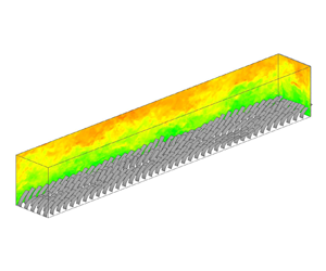
Figure 5. Snapshots of the flow field and canopy deformation for (a)  $Ca = 0$, (b) $Ca = 5$, (c) $Ca = 30$, (d) $Ca = 80$. The $x\unicode{x2013}y$ and $y\unicode{x2013}z$ planes show the streamwise velocity $u$ normalized by $u^*$.
The streamwise velocity in the channel increases as  $Ca$ increases because stems with greater flexibility are more prone to reduced drag owing to the reconfiguration of the stem (Vogel Reference Vogel1984; Gosselin, De Langre & MacHado-Almeida Reference Gosselin, De Langre and MacHado-Almeida2010; Shelley & Zhang Reference Shelley and Zhang2011; Pan et al. Reference Pan, Follett, Chamecki and Nepf2014b). For flexible canopies $(Ca \neq 0)$, the canopy top has a wave shape that propagates downstream; this phenomenon is known as ‘monami’ (Inoue Reference Inoue1955; Ackerman & Okubo Reference Ackerman and Okubo1993; Ghisalberti & Nepf Reference Ghisalberti and Nepf2002). The streamwise velocity contours in figure 5(b–d) reveal coherent structures in the flow. The distribution of these coherent flow structures and the monami wave phase appear to correspond to one another. As marked in figure 5(b), the location where the streamwise velocity is high (low) corresponds to stems with large (small) deformation. These observations are consistent with the common view that monami is generated by the interaction between coherent structures in the mixing layer and the deformable canopy (Ikeda & Kanazawa Reference Ikeda and Kanazawa1996; Ghisalberti & Nepf Reference Ghisalberti and Nepf2002; Nepf Reference Nepf2012). While the coherent structures cannot be observed via canopy deformation in the rigid canopy case, they can still be observed from the flow field. Note that in figure 5(a), there are two centres of low-speed velocity regions over the canopy and located at $x/h \sim 7$ and $x/h \sim 17$, respectively, which indicates coherent structures.
3.2. Velocity and Reynolds shear stress profiles
Figure 6 shows the vertical profiles of the mean streamwise velocity  $\langle \bar {u} \rangle$ and Reynolds shear stress $-\langle \overline {u^\prime v^\prime }\rangle$. All the mean velocity profiles have inflection points, which is characteristic of the velocity profiles in plane mixing layers (Pope Reference Pope2000). Table 4 provides the location of the inflection point for each $Ca$ case. Considering that the inflection point triggers flow instability in the plane mixing layer, we use the location of this inflection point to define the hydrodynamic canopy height, $h_c$, which we utilize to partition the regions inside and outside of the canopy. In the following discussion of canopy flow, we use $h_c$ as the default canopy height unless otherwise specified. Figure 6(b) demonstrates that the Reynolds shear stress follows the line $-\langle \overline {u^\prime v^\prime }\rangle /u^{*2} = 1-y/H$ above the maximum value near $h_c$, indicating that the transport of momentum by molecular viscosity is relatively small compared with the turbulent transport; below the maximum value, $-\partial \langle \overline {u^\prime v^\prime }\rangle /\partial y > 0$ due to canopy drag.

Figure 6. Vertical profiles of the (a) mean streamwise velocity  $\langle \bar {u} \rangle$ normalized by $u^*$ and (b) Reynolds shear stress $-\langle \overline {u^\prime v^\prime }\rangle$ normalized by ${u^*}^2$ for $Ca = 0, 5, 30$ and $80$. The inflection points on the velocity profiles are denoted by dots.
Table 4. Various characteristic statistics in the canopy flow: the height of the inflection point on the mean streamwise velocity profile,  $h_c$; the average stem tip height, $h_t$; the normalized difference between $h_c$ and $h_t$, $(h_c-h_t)/h$; the standard deviations of the stem tip displacements in the horizontal and vertical directions, $(\sigma _x, \sigma _y)$; and the skewness of the stem tip displacements in the vertical direction, $\tilde {\mu }_{3,y}$. Here $h_c$ and $h_t$ are also defined as the hydrodynamic canopy height and geometric canopy height, respectively.

3.3. Stem deformation and monami
We quantify the standard deviations of the stem tip displacements in the horizontal and vertical directions,  $(\sigma _x, \sigma _y)$, for flexible canopies. The results are shown in table 4. As $Ca$ increases, the stems clearly fluctuate with a smaller amplitude, a behaviour that increasingly resembles a rigid stem. This phenomenon occurs because a highly flexible stem yields more to the incoming flow, limiting its deformation fluctuation amplitude. We call this phenomenon ‘high flexibility-induced rigidity’ and use it to explain the similarity between the cases of $Ca = 0$ and 80, which are different from the cases of $Ca = 5$ and 30, in many discussions below. Note that this expression only reflects the similarity of rigid and highly flexible canopies in reconfiguration amplitude and does not imply material rigidity; the highly flexible canopy is still more sensitive to the turbulence of the flow than the less flexible canopy. We further examine the standard deviation of $x$ and $y$ displacements $(\sigma _x, \sigma _y)$ along the stem length to study the vibration mode of the stem. For undamped systems, each vibration mode is associated with one of its natural frequencies. The lowest natural frequency, also known as the fundamental natural frequency, is associated with the first vibration mode where there is no node along the standing wave. Higher natural frequencies, also known as harmonics, correspond to standing waves where there are one or more nodes (Blevins & Plunkett Reference Blevins and Plunkett1980). The result is shown in figure 7. Both $\sigma _x$ and $\sigma _y$ increase from the clamped end to the free end for all the cases, indicating the dominance of the first vibration mode. For $Ca = 5$, there is no inflection point along the profile, which means that the vibration mode is purely the first mode (Tschisgale et al. Reference Tschisgale, Löhrer, Meller and Fröhlich2021). For $Ca = 30$ and 80, at least one inflection point can be found along the profile, indicating that high vibration modes are also present.

Figure 7. Standard deviation of the (a)  $x$ displacement, $\sigma _x$, and (b) $y$ displacement, $\sigma _y$, along the stem length. Here $s/h$ denotes the stem coordinate, where $s/h = 0$ and $s/h = 1$ indicate the clamped and free ends, respectively.
The probability density function (p.d.f.) of the filament tip height  $y_{tip}/h$ is depicted in figure 8. As shown, the distribution of the filament tip height is not Gaussian: the $Ca = 5$ case has a negative skewness, and $Ca = 30$ and 80 show a positive skewness. The values of skewness $\sigma _y/h$ are given in table 4.

Figure 8. The p.d.f. of the filament tip height  $y_{tip}/h$.
The average stem tip height  $h_t$ is also given in table 4. Because $h_t$ is convenient to measure experimentally, we use it to define the geometric canopy height. By comparing the stem tip height $h_t$ with the hydrodynamic canopy height $h_c$ in the flexible canopy cases, it is found that whether $h_c$ or $h_t$ is larger is correlated with the skewness: for $Ca = 5$ where the skewness is negative, $h_c > h_t$; for $Ca = 30$ and 80 where the skewness is positive, $h_c < h_t$. This can be understood as being that negative (positive) skewness means more than half of the samples have the values higher (lower) than the average value, such that the hydrodynamic canopy height is higher (lower) than the average stem tip height. Therefore, the hydrodynamic canopy height is determined by the general distribution of the stem height, not merely the average stem height. As $Ca$ increases, the difference between $h_c$ and $h_t$ decreases. The normalized $(h_c-h_t)/h$ is also provided in table 4.
Next, the wavenumber and frequency–wavenumber spectra of the stem tip envelope are analysed to quantify the kinematic properties of monami. Our temporal sampling length  $T_s/(h/u^*)$ and sampling interval $t_s/(h/u^*)$ are 150 and 0.1, respectively, and the spatial sampling length and sampling interval follow the streamwise domain size $L_x/h = 20$ and the average interval between two filaments $L_x/(N_xh) = 0.5$, respectively. We denote the height of the stem tip as a function of the horizontal coordinates and time as $y_t(x,z,t)$; then, its wavenumber spectrum is
 \begin{equation} e_w(k_x) = \frac{1}{L_x L_z T}\int_{0}^{T}\int_{0}^{L_z}\int_{0}^{L_x} [y_t^\prime(x,z,t)]^2 {\rm e}^{-{\rm i}\,k_x x} \,\mathrm{d} x \,\mathrm{d}z \,\mathrm{d}t, \end{equation}
and its frequency–wavenumber spectrum is
 \begin{equation} e_{fw}(k_x,\omega) = \frac{1}{L_x L_z T}\int_{0}^{T}\int_{0}^{L_z}\int_{0}^{L_x} [y_t^\prime(x,z,t)]^2 {\rm e}^{-{\rm i}\,k_x x} {\rm e}^{-{\rm i}\,\omega t} \,\mathrm{d} x \,\mathrm{d}z \,\mathrm{d}t. \end{equation}
 Figure 9 shows the wavenumber spectra. Note that here the ‘energy’ is defined as  $y_t^{\prime 2}$; it only reflects the envelop geometry of the monami and is not proportional to the kinetic energy in the stems and turbulent flow. For all cases, the energetic wavenumber components are near $k_x h \sim 0.6$. We define this scale as the ‘monami scale’, which corresponds to the scale of the coherent structures in the mixing layer. Likewise, figure 10 depicts the frequency–wavenumber spectra for all cases. At every wavenumber, we define a characteristic frequency, $\omega _c(k_x)$, as
 \begin{equation} \omega_c(k_x) = \text{arg}\, \underset{\omega}{\max}[e_{fw}(k_x,\omega)]. \end{equation}
The extracted monami dispersion relation  $\omega _c(k_x)$ is plotted in figure 10(a–c) and compared in figure 10(d). Although the data are not smooth due to the limitation associated with high computational cost, the relation between the wavenumber and frequency is found to be nearly linear for all cases. All the cases have similar dispersion relations, i.e. similar wave phase speeds, with $c/u^* \sim 3$, where $c = \omega _c/k_x$. The monami phenomenon in all the cases can thus be categorized as a ‘slow wave’ or ‘young wave’ in the context of wind–wave interactions, where $c/u^* \lesssim 15$ (Belcher & Hunt Reference Belcher and Hunt1998). For the slow water waves, two different mechanisms may contribute to the momentum transfer process from the wind to the wave, including the singularity at the critical layer, defined as the height where $\langle u \rangle - c = 0$ (Miles Reference Miles1957), and the non-separated sheltering mechanism associated with the thickened boundary layer on the leeside of wave crest (Belcher & Hunt Reference Belcher and Hunt1993). While both mechanisms can induce an asymmetric pressure distribution on the wave surface, for slow water waves, the critical layer is close to the wave surface and thus does not play a significant role in the wave growth (Belcher & Hunt Reference Belcher and Hunt1998; Yang & Shen Reference Yang and Shen2010).

Figure 9. Wavenumber spectra of monami as defined by (3.1) for cases with  $Ca = 5, 30$ and 80.

Figure 10. Frequency–wavenumber spectra for monami as defined by (3.2) for cases with (a)  $Ca$ = 5, (b) $Ca$ = 30 and (c) $Ca$ = 80, where the black curves indicate the dispersion relation and the dashed line indicates the monami scale $k_m$. The dispersion relations for all the cases are compared in (d).
3.4. Conditional averages of the flow velocity and canopy drag
In this section, we illustrate the flow structures associated with the phases of monami. Different from water waves with long-lasting wave trains and continuous wave phases, for monami, the wave train is short and transient, which makes it difficult to identify the wave phase. Therefore, instead of quantifying the monami wave phase and analysing the associated flow field directly, we perform averaging conditioned upon the stem kinematic events corresponding to particular monami wave phases. Figure 11 illustrates a sketch of the correspondence between the stem kinematic events and the monami wave phases. We define four categories of events associated with the stem kinematics: (1) small deformation events, which occur when a stem has a large tip height and thus corresponds to the wave crest; (2) large backward speed events, which occur when a stem tip has a large negative horizontal velocity component and thus corresponds to the leeward surface; (3) large deformation events, which occur when a stem has a small tip height and thus corresponds to the wave trough; and (4) large forward speed events, which occur when a stem tip has a large positive horizontal velocity component and thus corresponds to the windward surface. We tested several other definitions, but they yielded similar results; for example, for a large backward speed event, we tested the definitions of a stem tip that has a large positive vertical velocity component and a stem tip that moves backward with a large negative horizontal velocity component.

Figure 11. Schematics of the relationship between the conditionally averaged events and the monami wave phase. The green lines represent the stems. The red arrows represent the velocities of the stem tips. The monami is represented by the black envelope connecting the stem tips and travels to the right.
We perform conditional averages on the above four categories of events and assemble the results to construct an overview of the flow structure associated with the monami phenomenon. The conditional average of a flow variable  $\phi (x,y,z,t)$ associated with a stem kinematic event is calculated by
 \begin{equation} \langle{\phi}\rangle^c(x,y,z) = \dfrac{1}{N}\sum_{i = 1}^{N} \phi(x_i,y_i,z_i,t_{{root},i}), \end{equation}
where  $x_i = (x-x_{{root},i}) \bmod L_x$; $y_i = y$; $z_i = (z-z_{{root},i}) \bmod L_z$; $(x_{{root},i}, z_{{root},i})$ and $t_{{root},i}$ $(i = 1,\ldots,N)$ are the horizontal coordinates of the root (i.e. the centre point of the clamp line at the base of the stem) and time, respectively, of the stem at which event $i$ occurs; $N$ is the total number of events; and ‘ $\bmod$’ is the binary modulo operator defined as $a \bmod b = a - b\lfloor a/b \rfloor$. Note that the modulo operation is performed in the streamwise and spanwise directions because both directions employ the periodic boundary condition, and by performing the modulo operation, the point $(x,z)$ where $x \in (-\infty,0) \cup [L_x,\infty )$ and $z \in (-\infty,0) \cup [L_z,\infty )$ can be translated into the computational domain. The above procedure of conditional averaging guarantees that the root of the stem experiencing the concerned event always translates to $(x,z) = (0,0)$ in the conditionally averaged flow field. The conditional average of the stem geometry $\langle {\boldsymbol \psi }\rangle ^c_{(x,z)}(s)$ is calculated as
 \begin{equation} \langle{\boldsymbol\psi}\rangle^c_{(x,z)}(s) = \dfrac{1}{N}\sum_{i = 1}^{N} \boldsymbol\psi_{(x_i,z_i)}(s,t_{{root},i}), \end{equation}
where  $s$ is the arclength coordinate and $\boldsymbol \psi _{(x,z)}(s,t)$ is the Eulerian coordinate of Lagrangian point $s$ on the stem rooted at $(x,z)$ at time $t$. To compute the conditional average, we take $N_s = 1500$ time frames of the flow field and select $r_s = 0.5\,\%$ of all the stem samples for each category of events. Therefore, for each category of events, the total number of samples is $N = N_s r_s N_f = 1500$, where $N_f = 200$ is the number of stems in the flow. Given that the subsample is large enough for statistics, further increasing the size of the subsample is not desirable because samples that are less representative will be included. For example, for the large deformation event, enlarging the subsample will include the samples with fewer deformations.
Next, we present the conditional average results. The conditional average of the streamwise velocity component  $u$ in the $x$–
$x$– $y$ plane that cuts through the centre of the stem row is given in figure 12. The relationship between the conditionally averaged events and the monami wave phase can be seen from the shape of the conditionally averaged canopy geometry calculated using (3.5). Near the canopy top, the contour lines of $u$ are approximately parallel to the canopy envelope. The trough of the flow streamlines over the stems exhibiting large deformation has a high streamwise velocity, which agrees with the argument that sweep events are associated with canopy deformation during monami (Ghisalberti & Nepf Reference Ghisalberti and Nepf2002, Reference Ghisalberti and Nepf2006; Okamoto & Nezu Reference Okamoto and Nezu2009; Patil & Singh Reference Patil and Singh2010). Inside the canopy, there are regions with negative $u$ immediately behind stems due to the backflow, and the size of these regions decreases as $Ca$ increases because of the smaller frontal area. These wake-scale flow structures may impact the transport of scalar quantities and particles, for example, by trapping them to elongate their residence time in the canopy.

Figure 12. Contours of the conditionally averaged normalized streamwise velocity  $\langle {u}\rangle ^c/u^*$ in the $x\unicode{x2013}y$ plane cutting through the centre of the stem row for (a,d,g,j) $Ca = 5$, (b,e,h,k) $Ca = 30$ and (c,f,i,l) $Ca = 80$. The conditionally averaged events are (a–c) small deformation events, (d–f) large forward speed events, (g–i) large deformation events and (j–l) large backward speed events. For the isopleths, the solid and dashed lines represent non-negative and negative values, respectively, and the intervals between non-negative values and between negative values are 0.5 and 0.1, respectively. The red lines represent the conditionally averaged shapes of the stems.
The streamlines of the conditionally averaged flow field in the monami-following frame are plotted in figure 13 to better illustrate the flow dynamics associated with the monami wave phase. Because all the cases with flexible canopies give similar results, only the case of  $Ca = 5$ is shown, where $c/u^* = 3$ is used. From the conditionally averaged flow fields for the large forward and large deformation speed events, we observe a vortex residing on the monami trough near $x/h = 0$ and $x/h = -0.5$, respectively. This vortex is similar to the cat's eye structure in wind–wave interactions (Lighthill Reference Lighthill1962; Sullivan, McWilliams & Moeng Reference Sullivan, McWilliams and Moeng2000; Yang & Shen Reference Yang and Shen2010), except that the streamlines extend into the canopy due to the permeability of the canopy. The vortex and the critical layer (where $\langle u\rangle ^c - c = 0$) reside near the canopy top, which is consistent with the result in § 3.3 that monami is a slow wave. The centre of the vortex, which is a convergence point, resides on the leeward surface. Another large vortex can be observed on the right; note that this vortex is stretched in the streamwise direction, and hence, only part of it is shown in the figure. A saddle point between these two vortices is located on the windward surface, as can be seen in figure 13(a), and the boundary between these two vortices can be identified from the saddle point and the influx streamlines connected to it. The streamlines above the vortices deform with them and thus are depressed above the saddle point. The streamlines of the conditionally averaged flow field in the monami-following frame are summarized in figure 14.

Figure 13. Streamlines of the conditionally averaged velocity field in the monami-following frame  $((\langle u\rangle ^c-c)/u^*, \langle v \rangle ^c/u^*)$ in the $x\unicode{x2013}y$ plane cutting through the centre of the stem row. The conditionally averaged events are (a) small deformation events, (b) large forward speed events, (c) large deformation events and (d) large backward speed events. The red lines represent the conditionally averaged shapes of the stems. The case of $Ca = 5$ is shown, where $c/u^* = 3$ is used.

Figure 14. Schematics of the flow pattern associated with the monami wave phase in the monami-following frame in the  $x$–
$x$– $y$ plane cutting through the centre of the stem row. The blue curves with arrows are streamlines. The red dashed lines indicate the boundaries between the main flow structures. The green lines and black curve represent the stems and the monami surface, respectively. The black cross indicates the saddle point.
Figure 15 shows the conditional average of the fluctuations of the streamwise and vertical velocity components,  $\langle {u^\prime }\rangle ^c$ and $\langle {v^\prime }\rangle ^c$, respectively. As all the flexible canopy cases show similar results, only the case of $Ca = 5$ is presented. For the streamwise velocity fluctuation $u^\prime$, we note that the large forward speed and large deformation events are characterized by $u^\prime > 0$. This phenomenon can be understood from two perspectives of the flow–stem interaction. First, from the perspective of the stems affecting the flow, highly deformed stems have smaller frontal areas, and stems with a large forward speed have a smaller velocity relative to the flow; in both situations, the flow resistance decreases, and the flow velocity is increased. Second, from the perspective of the flow affecting the stems, a faster flow can more easily deform the stems and maintain their large deformation. A similar explanation can be applied to $u^\prime < 0$ in small deformation and large backward speed events, where the frontal areas are large and the stems have a large velocity relative to the flow, thereby increasing the drag force, and a slow flow allows the stems to rebound. For the vertical velocity fluctuation $v^\prime$, the large forward speed and large deformation events are characterized by $v^\prime < 0$, while the small deformation and large backward speed events are characterized by $v^\prime > 0$. In summary, large forward speed and large deformation events are characterized by sweep events ( $u^\prime > 0, v^\prime < 0$), and small deformation and large backward speed events are characterized by ejection events ( $u^\prime < 0, v^\prime > 0$), which is consistent with the findings of previous experimental and numerical studies (Ghisalberti & Nepf Reference Ghisalberti and Nepf2006; Okamoto & Nezu Reference Okamoto and Nezu2009; Patil & Singh Reference Patil and Singh2010).

Figure 15. Contours of the conditionally averaged (a,c,e,g) normalized streamwise velocity fluctuation  $u^\prime /u^*$ and (b,d,f,h) normalized vertical velocity fluctuation $v^\prime /u^*$ in the $x\unicode{x2013}y$ plane cutting through the centre of the stem row. The conditionally averaged events are (a,b) small deformation events, (c,d) large forward speed events, (e,f) large deformation events and (g,h) large backward speed events. The red lines represent the conditionally averaged shapes of the stems. The case of $Ca = 5$ is shown.
Figure 16 shows the conditionally averaged fluctuations of the streamwise and vertical components of the drag force,  $\langle {f_1^\prime }\rangle ^c$ and $\langle {f_2^\prime }\rangle ^c$, respectively. Similar to figure 15, only the case of $Ca = 5$ is plotted, as it is representative of the flexible canopies. Within the stem oscillation trajectories, the time average of the streamwise force component $\bar {f}_1$ is always negative because it averages the zero value of $f_1$ if a stem is not present and the negative value of $f_1$ if a stem is present. As a result, for the region within the stem oscillation trajectories, $f_1^\prime$ is positive if a stem is not present because $f_1 = \bar {f}_1 + f_1^\prime$, $f_1 = 0$ and $\bar {f}_1 < 0$. When a stem is present, $f_1^\prime$ is usually negative. For example, for small deformation events (figure 16a), $f_1^\prime$ is negative around the stem tips in the centre of the domain. This is because this location is the highest reachable location of a stem, so $f_1$ ¡ 0 only for small deformation events and $f_1$ ¿ 0 otherwise. In contrast, for large deformation events (figure 16e), $f_1^\prime$ is negative at the upper part of the stems because the streamwise velocity there is higher than in other events (see figure 15), and therefore, the drag force has large negative values.

Figure 16. Contours of the conditionally averaged (a,c,e,g) normalized streamwise drag force fluctuation  $f_1^\prime /({u^{*}}^2/h)$ and (b,d,f,h) normalized vertical drag force fluctuation $f_2^\prime /({u^{*}}^2/h)$ in the $x\unicode{x2013}y$ plane cutting through the centre of the stem row. The conditionally averaged events are (a,b) small deformation events, (c,d) large forward speed events, (e,f) large deformation events and (g,h) large backward speed events. The red lines represent the conditionally averaged shapes of the stems. The case of $Ca = 5$ is shown.
For the vertical force component, its time average  $\bar {f}_2$ is positive within the stem oscillation trajectories because the inclination of the stems turns the streamwise incoming flow to the direction along the stem, with a positive vertical velocity component. Then, $f_2^\prime$ is negative if a stem is not present because $f_2 = \bar {f}_2 + f_2^\prime$, $f_2 = 0$ and $\bar {f}_2 > 0$. The sign of $f_2^\prime$ when a stem is present depends on the vertical velocity $v$ there. For large deformation and large forward speed events, sweep events near the stems have $v^\prime < 0$, which results in $f_2^\prime > 0$. In contrast, small deformation and large backward speed events have $f_2^\prime < 0$ near the stem tips and around the upper stem because of the ejection events with $v^\prime > 0$. The results shown in figures 15 and 16 are important for the analyses of the waving term in the TKE budget in § 4.6.
To summarize, in § 3 we study the flow structure, stem deformation and the dispersion relation of monami in the canopy flow. The monami wave speed  $c$ is found to be around $2u^*$, which is comparable to the wind over a slow water wave. Therefore, the flow features over the canopy, such as the cat's eye structure and the critical layer in the wave-following frame, are also similar. By performing conditional averaging according to the stem kinematics, we find that the backward and forward strokes of stems are associated with ejection and sweep events, respectively. From our stem-resolving simulation, detailed descriptions of the correlation between the velocity and drag associated with the monami are obtained, which are valuable for the analysis of the waving terms in the TKE and DKE budgets in the next section.
4. Spectral analyses of the TKE and DKE budgets
In this section, we perform spectral analyses of the TKE and DKE budgets. First, in § 4.1 the budget equation of TKE is derived, and the vertical profiles of TKE, DKE and TKE budget terms are compared for cases with different canopy flexibilities. Then, in § 4.2 the spectral budget equation of TKE for canopy flows is derived following the two-point correlation function approach in the previous studies of pure channel flows. Next, the terms in the spectral budget equation are analysed, including the TKE and production terms (§ 4.3), three wall-normal transport terms (§ 4.4), the intercomponent and interscale terms (§ 4.5) and the waving term associated with flexible stems (§ 4.6). In § 4.6, the spectral shortcut mechanism of the canopy flow is understood by comparing the interscale and waving terms. Also in § 4.6, the contributions of the velocity components and quadrant events to the waving term are studied, and the effects of the monami wave phases on the waving term are analysed by conditional averaging. Finally, in § 4.7 the spectral budget at the monami and wake scales are elucidated, from which a schematic on the energy flux in the canopy flow is obtained.
4.1. Energy transport in the canopy flow: mean kinetic energy, DKE and TKE
Following (2.20), the kinetic energy in the canopy flow  $e = \langle \overline {u_i u_i}\rangle /2$ can be decomposed into
 \begin{equation} e = \underbrace{\dfrac{1}{2} \langle \bar{u}_i \rangle \langle \bar{u}_i \rangle}_{e_{{MKE}}} + \underbrace{\dfrac{1}{2} \langle \bar{u}_i^{\prime\prime} \bar{u}_i^{\prime\prime}\rangle}_{e_{{DKE}}} + \underbrace{\dfrac{1}{2} \langle \overline{u_i^\prime u_i^\prime} \rangle}_{e_{{TKE}}}, \end{equation}
where  $e_{{MKE}}$, $e_{{DKE}}$ and $e_{{TKE}}$ are the mean kinetic energy (MKE), DKE and TKE, respectively. The DKE represents the part of the kinetic energy induced by the flow inhomogeneity and does not exist in a pure channel flow. The TKE budget in the canopy flow is (Finnigan Reference Finnigan2000)
 $$\begin{gather} \dfrac{\partial}{\partial t}\left(\dfrac{1}{2}\langle\overline{u_i' u_i'}\rangle\right) = \underbrace{\dfrac{1}{2}\langle\bar{u}_j\rangle\dfrac{\partial\langle\overline{u_i'u_i'} \rangle}{\partial x_j}}_{A} - \underbrace{\langle\overline{u_i' u_j'}\rangle\dfrac{\partial\langle\bar{u}_i\rangle}{\partial x_j}}_{P_s} - \underbrace{\left\langle\overline{u_i' u_j'}''\dfrac{\partial \bar{u}_i''}{\partial x_j}\right\rangle}_{P_w} - \underbrace{\dfrac{1}{2}\dfrac{\partial \langle\bar{u}_j''\overline{u_i'u_i'}''\rangle}{\partial x_j}}_{T_d}\nonumber\\ - \underbrace{\dfrac{1}{2}\dfrac{\partial \langle\overline{u_i'u_i'u_j'}\rangle}{\partial x_j}}_{T_t} - \underbrace{\dfrac{\partial \langle\overline{p'u_j'}\rangle}{\partial x_j}}_{T_p} + \underbrace{\dfrac{\nu}{2}\dfrac{\partial^2\langle\overline{u_i'u_i'}\rangle}{\partial x_j \partial x_j}}_{T_v} - \underbrace{\nu\left\langle\overline{\dfrac{\partial u_i'}{\partial x_j}\dfrac{\partial u_i'}{\partial x_j}}\right\rangle}_{\epsilon} + \underbrace{\langle\overline{f'u'}\rangle}_W, \end{gather}$$
where the right-hand side terms are the convection term  $A$, shear production term $P_s$, wake production term $P_w$, dispersive transport term $T_d$, turbulent transport term $T_t$, pressure transport term $T_p$, viscous transport term $T_v$, dissipation term $\epsilon$ and waving term $W$. In these terms, the convection term $A$ theoretically equals zero in the present problem set-up, the wake production term $P_w$ and the dispersive transport term $T_d$ are related to the spatial inhomogeneity of the canopy flow, and the waving term $W$ represents the correlation between the hydrodynamic drag and the stem waving motion. Note that the ‘waving term’ is not necessarily associated with the canopy waving motion; this term also exists in the rigid canopy where the stems do not wave. However, we still call it ‘waving term’ following the convention in the literature, such as (7.1) in Finnigan (Reference Finnigan2000). In the literature, fewer studies have been conducted on the waving term than on the other terms. Our numerical simulation provides comprehensive descriptions of the hydrodynamic drag and flow velocity in space and time such that the canopy waving effect can be quantified and analysed.
Figure 17 plots the vertical profiles of TKE and DKE. Below  $y \sim 1.8h$, TKE increases with $Ca$, and the height of its maximum value decreases as $Ca$ increases because the canopy height decreases. The maximum values of the TKE profiles are above the canopy where the centres of the coherent structures in the mixing layer are located (Nepf Reference Nepf2012). Above $y \sim 1.8h$, the TKE profiles of all the cases collapse into one curve, indicating that the TKE enhancement effect of flexible canopies is limited with height. The DKE is prominent only in the canopy region. The amplitude of DKE is small compared with that of TKE, which is consistent with the measurement result of Raupach, Coppin & Legg (Reference Raupach, Coppin and Legg1986). Interestingly, the maximum value of DKE in the rigid canopy is larger than that at $Ca = 5$ and closer to that in the cases of $Ca = 30$ and 80. We believe the reason is that the oscillation amplitude of the stems has a negative correlation with DKE and that highly flexible stems oscillate less and behave more like a rigid stem, i.e. the phenomenon of ‘high flexibility-induced rigidity’ as discussed in § 3.3.

Figure 17. Vertical profiles of the (a) TKE and (b) DKE averaged over time and over the  $x\unicode{x2013}z$ planes. Both TKE and DKE are normalized by ${u^*}^2$. The cases are: black solid line, $Ca = 0$; red dashed line, $Ca = 5$; green dashed–dotted line, $Ca = 30$; and blue dashed–dotted line, $Ca = 80$.
The vertical profiles of the TKE budget terms (4.2) are plotted in figure 18. For all cases, the shear production term  $P_s$ is the dominant energy source. However, the wake production term $P_w$ can be higher than $P_s$ inside the canopy because of the strong flow inhomogeneity there, which is consistent with the findings of Raupach et al. (Reference Raupach, Coppin and Legg1986) and Poggi et al. (Reference Poggi, Porporato, Ridolfi, Albertson and Katul2004). The turbulent transport term $T_t$ has the largest magnitude among all four transport terms and plays an important role in balancing the high energy production immediately above the canopy and the high dissipation inside the canopy. In the rigid canopy case, the extrema of $P_s$ and $\epsilon$ are $12 {u^*}^3/h$ and $-5 {u^*}^3/h$, respectively, which agree with the particle image velocimetry results of Yue et al. (Reference Yue, Meneveau, Parlange, Zhu, Kang and Katz2008), who measured a rigid canopy flow in a wind tunnel. The flexible canopy cases have a similar profile shape for each term, except that the terms have larger amplitudes and lower peak heights as $Ca$ increases owing to the lower canopy height and faster flow. Comparing the rigid and flexible canopy cases reveals that the peak of $P_s$ is sharper in the former because the oscillation of stems in the flexible canopies smears the canopy top and the flow shear there. Another major difference between the rigid and flexible canopy cases is the waving term $W$. For the rigid canopy case ( $W = \langle \overline {f'u'}\rangle = 0$), because $u = 0$ on the stem surface and $f = 0$ away from the stem surface, $u^\prime \neq 0$ and $f^\prime \neq 0$ cannot be satisfied simultaneously. For the flexible canopy cases, the waving term is an energy source near the canopy top where the stem tip has a large oscillation amplitude and a weak energy sink inside the canopy where the stem oscillation is reduced. The maximum value of $W$ is approximately half of $P_s$, which makes it another major TKE source term for the flexible canopy cases. Owing to the difficulty of experimentally measuring the drag–velocity correlation in flexible canopies, previous studies did not clarify the role of the waving term in canopy flow dynamics (Finnigan Reference Finnigan1979, Reference Finnigan2000; Raupach & Thom Reference Raupach and Thom1981). Our simulations, which explicitly resolve the stems, show that the waving term can play an important role in TKE generation in flexible canopies. More analyses of the waving effects are provided in the sections below.

Figure 18. Vertical profiles of the TKE budget terms defined in (4.2) inside and near the canopy top for (a)  $Ca = 0$, (b) $Ca = 5$, (c) $Ca = 30$, (d) $Ca = 80$. The terms are as follows: $P_s$, the shear production term; $P_w$, the wake production term; $T_d$, the dispersive transport term; $T_t$, the turbulent transport term; $T_p$, the pressure transport term; $T_v$, the viscous transport term; $\epsilon$, the dissipation term; and $W$, the waving term. All the terms are normalized by ${u^*}^3/h$.
4.2. Algorithm for the spectral analysis of the TKE budget
We perform a spectral analysis of the TKE budget following the two-point correlation function approach (Lee & Moser Reference Lee and Moser2015, Reference Lee and Moser2019; Wang et al. Reference Wang, Zhang, Hao, Huang, Shen, Xu and Zhang2020). Note that there is another equivalent approach that starts from the Navier–Stokes equations in the form of Fourier modes (Mizuno Reference Mizuno2016; Cho et al. Reference Cho, Hwang and Choi2018). We adopt the former approach, which is briefly described below. Considering the two-point correlation of  $u_i(x,y,z,t)$ and $\tilde {u}_j(x,r_x,y,z,t)=u_j(x+r_x,y,z,t), j=1,2,3$, the spectral budget of the Reynolds stress is
 $$\begin{gather} \dfrac{\partial
\langle{\overline{u_i^\prime
\tilde{u}_j^\prime}}\rangle_{x}}{\partial t}(r_x,y,z) =
\underbrace{\left(-\langle{\overline{\tilde{u}_j^\prime
u_k^\prime}}\rangle_{x}\dfrac{\partial\langle \bar{u}_i
\rangle_{x}}{\partial x_k} - \langle{\overline{u_i^\prime
\tilde{u}_k^\prime}}\rangle_{x}\dfrac{\partial\langle
\bar{u}_j \rangle_{x}}{\partial
\tilde{x}_k}\right)}_{{\mathsf{R}}_{ij}^P} \underbrace{-
\left\langle\overline{\tilde{u}_j^\prime \dfrac{\partial
u_k^\prime u_i^\prime}{\partial x_k} + u_i^\prime
\dfrac{\partial \tilde{u}_k^\prime
\tilde{u}_j^\prime}{\partial \tilde{x}_k}}
\right\rangle_x}_{{\mathsf{R}}_{ij}^T}\nonumber\\ \underbrace{-
\dfrac{1}{\rho} \left\langle\overline{\tilde{u}_j^\prime
\dfrac{\partial p^\prime}{\partial x_i} + u_i^\prime
\dfrac{\partial \tilde{p}}{\partial \tilde{x}_j}}
\right\rangle_x}_{{\mathsf{R}}_{ij}^\varPi} \underbrace{+ \nu
\left\langle\overline{\tilde{u}_j^\prime \dfrac{\partial^2
u_i^\prime}{\partial x_k \partial x_k} + u_i^\prime
\dfrac{\partial^2 \tilde{u}_j^\prime}{\partial \tilde{x}_k
\partial \tilde{x}_k}}\right\rangle_x}_{{\mathsf{R}}_{ij}^\nu} +
\underbrace{\langle\overline{\tilde{u}_j^\prime f_i^\prime
+ u_i^\prime \tilde{f}_j^\prime}\rangle_x}_{{\mathsf{R}}_{ij}^W},
\end{gather}$$
$$\begin{gather} \dfrac{\partial
\langle{\overline{u_i^\prime
\tilde{u}_j^\prime}}\rangle_{x}}{\partial t}(r_x,y,z) =
\underbrace{\left(-\langle{\overline{\tilde{u}_j^\prime
u_k^\prime}}\rangle_{x}\dfrac{\partial\langle \bar{u}_i
\rangle_{x}}{\partial x_k} - \langle{\overline{u_i^\prime
\tilde{u}_k^\prime}}\rangle_{x}\dfrac{\partial\langle
\bar{u}_j \rangle_{x}}{\partial
\tilde{x}_k}\right)}_{{\mathsf{R}}_{ij}^P} \underbrace{-
\left\langle\overline{\tilde{u}_j^\prime \dfrac{\partial
u_k^\prime u_i^\prime}{\partial x_k} + u_i^\prime
\dfrac{\partial \tilde{u}_k^\prime
\tilde{u}_j^\prime}{\partial \tilde{x}_k}}
\right\rangle_x}_{{\mathsf{R}}_{ij}^T}\nonumber\\ \underbrace{-
\dfrac{1}{\rho} \left\langle\overline{\tilde{u}_j^\prime
\dfrac{\partial p^\prime}{\partial x_i} + u_i^\prime
\dfrac{\partial \tilde{p}}{\partial \tilde{x}_j}}
\right\rangle_x}_{{\mathsf{R}}_{ij}^\varPi} \underbrace{+ \nu
\left\langle\overline{\tilde{u}_j^\prime \dfrac{\partial^2
u_i^\prime}{\partial x_k \partial x_k} + u_i^\prime
\dfrac{\partial^2 \tilde{u}_j^\prime}{\partial \tilde{x}_k
\partial \tilde{x}_k}}\right\rangle_x}_{{\mathsf{R}}_{ij}^\nu} +
\underbrace{\langle\overline{\tilde{u}_j^\prime f_i^\prime
+ u_i^\prime \tilde{f}_j^\prime}\rangle_x}_{{\mathsf{R}}_{ij}^W},
\end{gather}$$
where  $\langle {\cdot }\rangle _x$ indicates the average in the streamwise direction. In the above equation, ${\mathsf{R}}_{ij}^P$, ${\mathsf{R}}_{ij}^T$, ${\mathsf{R}}_{ij}^\varPi$, ${\mathsf{R}}_{ij}^\nu$ and ${\mathsf{R}}_{ij}^W$ are the shear production term, turbulent term, pressure term, viscous term and waving term, respectively. The terms ${\mathsf{R}}_{ij}^T$, ${\mathsf{R}}_{ij}^\varPi$ and ${\mathsf{R}}_{ij}^\nu$ can be further decomposed such that: ${\mathsf{R}}_{ij}^T$ can be decomposed into a wall-normal turbulent transport term ${\mathsf{R}}_{ij}^{{NTT}}$ and an interscale transport term ${\mathsf{R}}_{ij}^{{IST}}$,
 \begin{gather} {\mathsf{R}}_{ij}^{{NTT}} ={-}\frac{1}{2}\left(\dfrac{\partial \langle\overline{\tilde{u}_j^\prime u_i^\prime u_2^\prime}\rangle_x}{\partial y} + \dfrac{\partial \langle\overline{u_i^\prime \tilde{u}_j^\prime \tilde{u}_2^\prime}\rangle_x}{\partial y} \right), \end{gather}
 \begin{gather} \hspace{-3pc}{\mathsf{R}}_{ij}^{{IST}} =
\dfrac{\partial \langle\overline{\tilde{u}_j^\prime
u_i^\prime u_1^\prime}\rangle_x}{\partial r_x} -
\dfrac{\partial \langle\overline{u_i^\prime
\tilde{u}_j^\prime \tilde{u}_1^\prime}\rangle_x}{\partial
r_x} + \dfrac{\partial \langle\overline{\tilde{u}_j^\prime
u_i^\prime u_3^\prime}\rangle_x}{\partial z} -
\dfrac{\partial \langle\overline{u_i^\prime
\tilde{u}_j^\prime \tilde{u}_3^\prime}\rangle_x}{\partial
z} \nonumber\\ \hspace{5.3pc}-\frac{1}{2}\left(\dfrac{\partial
\langle\overline{\tilde{u}_j^\prime u_i^\prime
u_2^\prime}\rangle_x}{\partial y} + \dfrac{\partial
\langle\overline{u_i^\prime \tilde{u}_j^\prime
\tilde{u}_2^\prime}\rangle_x}{\partial y} \right) +
\left\langle\overline{u_i^\prime u_2^\prime \dfrac{\partial
\tilde{u}_j^\prime}{\partial y}}\right\rangle_x +
\left\langle\overline{\tilde{u}_j^\prime \tilde{u}_2^\prime
\dfrac{\partial u_j^\prime}{\partial
y}}\right\rangle_x ;
\end{gather}
\begin{gather} \hspace{-3pc}{\mathsf{R}}_{ij}^{{IST}} =
\dfrac{\partial \langle\overline{\tilde{u}_j^\prime
u_i^\prime u_1^\prime}\rangle_x}{\partial r_x} -
\dfrac{\partial \langle\overline{u_i^\prime
\tilde{u}_j^\prime \tilde{u}_1^\prime}\rangle_x}{\partial
r_x} + \dfrac{\partial \langle\overline{\tilde{u}_j^\prime
u_i^\prime u_3^\prime}\rangle_x}{\partial z} -
\dfrac{\partial \langle\overline{u_i^\prime
\tilde{u}_j^\prime \tilde{u}_3^\prime}\rangle_x}{\partial
z} \nonumber\\ \hspace{5.3pc}-\frac{1}{2}\left(\dfrac{\partial
\langle\overline{\tilde{u}_j^\prime u_i^\prime
u_2^\prime}\rangle_x}{\partial y} + \dfrac{\partial
\langle\overline{u_i^\prime \tilde{u}_j^\prime
\tilde{u}_2^\prime}\rangle_x}{\partial y} \right) +
\left\langle\overline{u_i^\prime u_2^\prime \dfrac{\partial
\tilde{u}_j^\prime}{\partial y}}\right\rangle_x +
\left\langle\overline{\tilde{u}_j^\prime \tilde{u}_2^\prime
\dfrac{\partial u_j^\prime}{\partial
y}}\right\rangle_x ;
\end{gather} ${\mathsf{R}}_{ij}^{\varPi }$ can be decomposed into a wall-normal pressure transport term ${\mathsf{R}}_{ij}^{{NPT}}$ and an intercomponent transport term ${\mathsf{R}}_{ij}^{{ICT}}$,
 \begin{gather} {\mathsf{R}}_{ij}^{{NPT}} = \frac{1}{\rho}\left(\dfrac{\partial \langle\overline{\tilde{u}_j^\prime p^\prime}\rangle_x}{\partial y}\delta_{i2} + \dfrac{\partial \langle\overline{u_i^\prime \tilde{p}^\prime}\rangle_x}{\partial y}\delta_{j2} \right), \end{gather}
 \begin{gather} {\mathsf{R}}_{ij}^{{ICT}} ={-}\frac{1}{\rho}\left\langle\overline{p^\prime \dfrac{\partial \tilde{u}_j^\prime}{\partial \tilde{x}_i}} + \tilde{p}^\prime \dfrac{\partial u_i^\prime}{\partial x_j}\right\rangle_x; \end{gather} ${\mathsf{R}}_{ij}^{\nu }$ can be decomposed into a wall-normal viscous transport term ${\mathsf{R}}_{ij}^{{NVT}}$ and a dissipation term ${\mathsf{R}}_{ij}^{{DIS}}$,
 \begin{gather} {\mathsf{R}}_{ij}^{{NVT}} = \nu \dfrac{\partial^2 \langle\overline{u_i^\prime \tilde{u}_j^\prime}\rangle_x}{\partial y \partial y}, \end{gather}
 \begin{gather} {\mathsf{R}}_{ij}^{{DIS}} ={-}2\nu\left\langle\overline{\dfrac{\partial u_i^\prime}{\partial r_x}\dfrac{\partial \tilde{u}_j^\prime}{\partial r_x} + \dfrac{\partial u_i^\prime}{\partial y}\dfrac{\partial \tilde{u}_j^\prime}{\partial y} + \dfrac{\partial u_i^\prime}{\partial z}\dfrac{\partial \tilde{u}_j^\prime}{\partial z}}\right\rangle_x. \end{gather}
Therefore, we have
 \begin{equation} \dfrac{\partial \langle{\overline{u_i^\prime \tilde{u}_j^\prime}}\rangle_{x}}{\partial t}(r_x,y,z) = {\mathsf{R}}_{ij}^{P} + {\mathsf{R}}_{ij}^{{NTT}} + {\mathsf{R}}_{ij}^{{IST}} + {\mathsf{R}}_{ij}^{{NPT}} + {\mathsf{R}}_{ij}^{{ICT}} + {\mathsf{R}}_{ij}^{{NVT}} + {\mathsf{R}}_{ij}^{{DIS}} + {\mathsf{R}}_{ij}^W. \end{equation}
By taking the trace of this equation ( $i=j$), performing the Fourier transform about $r_x$ while applying the Wiener–Khinchin theorem and averaging in the spanwise direction, we can obtain
 \begin{equation} \dfrac{\partial E_e}{\partial t}(k_x,y) = E_P + E_{{NTT}} + E_{{NPT}} + E_{{NVT}} + E_{{IST}} + E_{{DIS}} + E_{W}, \end{equation}
where  $k_x$ is the streamwise wavenumber, $E_e$ is the streamwise spectrum of TKE, and the right-hand side terms are the shear production $E_P$, wall-normal turbulent transport $E_{{NTT}}$, wall-normal pressure transport $E_{{NPT}}$, wall-normal viscous transport $E_{{NVT}}$, interscale transport $E_{{IST}}$, dissipation $E_{{DIS}}$ and waving effect $E_W$, respectively. The definitions of these terms are as follows:
 \begin{gather} E_e = \mathrm{Re} \left[\left\langle\overline{\mathcal{F}^*(u_i^\prime) \mathcal{F}(u_i^\prime)}\right\rangle_z\right], \end{gather}
 \begin{gather}E_P = \mathrm{Re} \left[{-}2\left\langle\overline{\mathcal{F}^*(u_k^\prime \dfrac{\partial \bar{u}_i}{\partial x_k}) \mathcal{F}(u_i^\prime)}\right\rangle_z\right], \end{gather}
 \begin{gather}E_{{NTT}} = \mathrm{Re} \left[\dfrac{\partial}{\partial y}\left\langle\overline{\mathcal{F}^*(u_i^\prime u_2^\prime) \mathcal{F}(u_i^\prime)}\right\rangle_z\right], \end{gather}
 \begin{gather}E_{{NPT}} = \mathrm{Re} \left[-\dfrac{2}{\rho}\left\langle\overline{\mathcal{F}^*(p^\prime) \mathcal{F}(u_2^\prime)}\right\rangle_z\right], \end{gather}
 \begin{gather}E_{{NVT}} = \mathrm{Re} \left[\nu\dfrac{\partial^2}{\partial y^2}\left\langle\overline{\mathcal{F}^*(u_i^\prime) \mathcal{F}(u_i^\prime)}\right\rangle_z\right], \end{gather}
 \begin{gather} \hspace{-3pc}E_{{IST}} = \mathrm{Re} \left[{-}2ik_x\left\langle\overline{\mathcal{F}^*(u_i^\prime u_1^\prime) \mathcal{F}(u_i^\prime)}\right\rangle_z - \dfrac{\partial}{\partial y}\left\langle\overline{\mathcal{F}^*(u_i^\prime u_2^\prime) \mathcal{F}(u_i^\prime)}\right\rangle_z\right. \nonumber\\ \hspace{2pc}+ \left.2\left\langle\overline{\mathcal{F}^*(u_i^\prime u_2^\prime) \mathcal{F}(\dfrac{\partial u_i^\prime}{\partial y})}\right\rangle_z + 2\left\langle\overline{\mathcal{F}^*(u_i^\prime u_3^\prime) \mathcal{F}(\dfrac{\partial u_i^\prime}{\partial z})}\right\rangle_z\right], \end{gather}
 \begin{gather}E_{{DIS}} = \mathrm{Re} \left[{-}2\nu k_x^2 \left\langle\overline{\mathcal{F}^*(u_i^\prime) \mathcal{F}(u_i^\prime)}\right\rangle_z - 2\nu \left\langle\overline{\mathcal{F}^*\left(\dfrac{\partial u_i^\prime}{\partial y}\right) \mathcal{F}\left(\dfrac{\partial u_i^\prime}{\partial y}\right)}\right\rangle_z \right]\nonumber\\ \hspace{-4pc}- \left. 2\nu \left\langle\overline{\mathcal{F}^*\left(\dfrac{\partial u_i^\prime}{\partial z}\right) \mathcal{F}\left(\dfrac{\partial u_i^\prime}{\partial z}\right)}\right\rangle_z \right], \end{gather}
 \begin{gather}E_{{W}} = \mathrm{Re} \left[2\left\langle\overline{\mathcal{F}^*(f_i^\prime) \mathcal{F}(u_i^\prime)}\right\rangle_z\right], \end{gather}
where  $\langle {\cdot }\rangle _z$ represents the spanwise average, $\mathcal {F}$ is the Fourier transform operator, $({\cdot })^*$ is the complex conjugate operator and $\mathrm {Re}({\cdot })$ takes the real part of a complex number. The correspondence of ${\mathsf{R}}_{ij}^{{ICT}}$ in (4.10), $\boldsymbol {E}_{{ICT}}$, has the form of
 \begin{equation} E_{{ICT},i} = \mathrm{Re} \left[\dfrac{2}{\rho}\left\langle\overline{\mathcal{F}^*(p^\prime) \mathcal{F}\left(\dfrac{\partial u_i^\prime}{\partial x_i}\right)}\right\rangle_z\right], \quad \text{no summation, }i = 1, 2, \text{or } 3, \end{equation}
where  $i$ indicates the component. Note that $\boldsymbol {E}_{{ICT}}$ does not exist in (4.11), because it transfers energy only among the three velocity components, such that
 \begin{equation} E_{ICT,1}(k_x,y) + E_{ICT,2}(k_x,y) + E_{ICT,3}(k_x,y) = 0. \end{equation}
Here, we consider only the streamwise Fourier modes because we focus on the interaction between the canopy and the streamwise structure of the coherent vortices in the mixing layer. Spanwise Fourier modes need to be considered when studying the spanwise structure, which is important for other types of flows (see, e.g. Cho et al. Reference Cho, Hwang and Choi2018) but is less important than the dominant streamwise structures in canopy flows. In the following analyses of the TKE budget terms, we compare our results mainly with the slow-wave case ( $c/u^* = 2$) in Wang et al. (Reference Wang, Zhang, Hao, Huang, Shen, Xu and Zhang2020), where the spectral TKE budget for a 3-D turbulent airflow over water waves is analysed, and has the closest simulation set-up in the literature with our canopy problem for spectral TKE budget analysis. Note that because the velocity fluctuations in Wang et al. (Reference Wang, Zhang, Hao, Huang, Shen, Xu and Zhang2020) contain both turbulent and wave-coherent components, which are equivalent to the combination of the turbulent and dispersive components in our case, their TKE budget is equivalent to the sum of the TKE and DKE budgets in our case. Because the DKE budget is non-trivial only at the wake scale, our TKE budget can still be compared with their results, but not at the wake scale. In the following sections §§ 4.3–4.6, we first discuss the TKE budget in the spectral space at various heights, followed by a discussion of the vertical profiles of the TKE and DKE budgets at the monami and wake scales in § 4.7.
4.3. Spectra of TKE and the production term
Figure 19 shows the streamwise spectra of TKE,  $E_e$. The TKE is higher at low wavenumbers and over the canopy and achieves the largest value near the canopy top. As the canopy flexibility increases, the TKE maximum value increases, and the height of the maximum value decreases as the canopy height decreases. These variations are consistent with figure 17(a). From the spectra, we can identify two significant spatial scales that do not exist in the boundary layer spectrum (de Langre Reference de Langre2008). The first scale is approximately $k_x h \sim 4{\rm \pi}$, where the TKE inside the canopy reaches a local maximum value, as indicated in figure 19. This scale corresponds to the interval between adjacent stems and hence represents the characteristic scale of the wake behind the stems, consistent with the observation by Olivieri et al. (Reference Olivieri, Brandt, Rosti and Mazzino2020). We call this scale the ‘wake scale’ with a wavenumber $k_w$. The local maximum TKE is consistent with the spectral shortcut mechanism (Kaimal & Finnigan Reference Kaimal and Finnigan1994; Finnigan Reference Finnigan2000; Olivieri et al. Reference Olivieri, Brandt, Rosti and Mazzino2020). It should be noted that such a local maximum TKE also exists at the integer multipliers of the wake scale, also known as the harmonics (not plotted in the figures), and its amplitude decreases as the multiplier increases. These harmonics can also be observed in the results of Wang et al. (Reference Wang, Zhang, Hao, Huang, Shen, Xu and Zhang2020), who showed that the streamwise spectrum of the TKE for air turbulence over a slow water wave exhibits high TKE at the dominant wavelength scale and harmonics at higher wavenumbers. The second significant scale is approximately $k_x h \sim 0.6$. For clarity, figure 20 plots locally magnified views of figure 19 to highlight the low wavenumber range of $k_x h \leq 5$ in the lower part of the channel ( $y/h \leq 1$). For every case, close to the channel bottom wall, there exists a local maximum TKE near $k_x h \sim 0.6$; this is also the global maximum except in the case of $Ca = 80$, where the spatially averaged component at $k_x h \sim 0$ is higher. Note that $k_x h \sim 0.6$ corresponds to the energetic wavenumber component of the monami, as shown in figure 9, at which the coherent flow structure near the canopy top influences the lower canopy. We call this scale the ‘monami scale’ with a wavenumber $k_m$. Two reasons can explain why the local maximum value at the monami scale occurs close to the channel bottom. One is due to the penetration of the shear vortices into the canopy. The other reason is that the flow close to the channel bottom, therefore within the canopy, directly interacts with the monami, such that the monami scale is more prominent than the flow outside the canopy where there is no direct flow–canopy contact. The wake and monami scales represent the characteristic large flow scale of the coherent structures in the mixing layer and the small flow scale of the wakes behind the stems, respectively. Note that previous experimental studies usually measured the temporal spectra and then obtained the spatial spectra based on Taylor's frozen hypothesis to discuss the spectral shortcut (e.g. Allen Reference Allen1968; Seginer et al. Reference Seginer, Mulhearn, Bradley and Finnigan1976; Brunet et al. Reference Brunet, Finnigan and Raupach1994; Kaimal & Finnigan Reference Kaimal and Finnigan1994). We plot the temporal spectra of TKE at the canopy height for each case. Note that owing to the limitation of the simulation time duration, the temporal spectrum obtained at one point is very noisy. Therefore, we averaged the temporal spectra at all grid nodes over the canopy height $h_c$, and the result is plotted in figure 21. As shown, there are two local maxima for each case. One is located at $\omega h/u^* \sim 1.6$, which corresponds to the monami scale, and the other is located around $\omega h/u^* \sim 28$, which corresponds to the wake scale. Considering that our simulation can precisely capture the spatial variation, we hereinafter discuss the spectral shortcut in the context of spatial spectra. In the following sections, the flow features at these two scales and the interaction between them are analysed and discussed.

Figure 19. The 1-D streamwise spectra of TKE,  $E_{e}$, for (a) $Ca$ = 0, (b) $Ca$ = 5, (c) $Ca$ = 30, (d) $Ca$ = 80. The term is normalized by ${u^*}^2/h^2$. Here $k_m$ and $k_w$ are denoted by arrows on the horizontal axis.

Figure 20. Magnified view of figure 19 for  $k_x h \leq 5$ and $y/h \leq 1$: (a) $Ca$ = 0; (b) $Ca$ = 5; (c) $Ca$ = 30; (d) $Ca$ = 80. The increment is 0.005 between contour lines from 0 to 0.2. Here $k_m$ is denoted by an arrow on the horizontal axis.

Figure 21. Averaged one-point temporal spectra over the canopy height for  $Ca = 0, 5, 30$ and 80.
To further understand the source of TKE at different streamwise wavenumbers, the streamwise spectra of the shear production term  $E_P$ are shown in figure 22. Similar to the spectra for the TKE, $E_P$ attains its largest value near the canopy top where the shear is strong and is high at low wavenumbers, especially at the monami scale (Finnigan Reference Finnigan2000). Local maximum values also exist at the wake scale, but the heights of the regions featuring prominent values differ among the cases: for the rigid canopy, there is only one region near the canopy top ( $y/h \sim 1$), whereas for the flexible canopies, there is another region near the channel bottom. We believe that this discrepancy is caused by the different heights of the primary shear. For the rigid canopy ( $Ca = 0$), the velocity difference across the canopy top is high and the velocity inside the canopy is low, so the primary shear occurs at the canopy top. As the canopy becomes more flexible, the boundary between the flows inside and outside the canopy becomes less defined because the oscillation of the stems weakens the shear at the canopy top. At the same time, the flow velocity inside the canopy increases as the drag coefficient decreases owing to the reconfiguration of the stems, and thus, the shear at the channel bottom is strong. The shear strength is indicated by the vertical gradient of the streamwise flow velocity $\partial \langle \bar {u} \rangle /\partial y$ and is observable from figure 6(a), where $Ca = 0$ has a high streamwise velocity gradient at the canopy top and $Ca = 30$ and $80$ have a high streamwise velocity gradient close to the channel bottom wall.

Figure 22. The 1-D streamwise spectra of the production term  $E_{P}$ for (a) $Ca = 0$, (b) $Ca = 5$, (c) $Ca = 30$, (d) $Ca = 80$. The term is normalized by ${u^*}^3/h^3$. Here $k_m$ and $k_w$ are denoted by arrows on the horizontal axis.
Note that some previous studies found regions with negative shear production in spectral analyses of the TKE budget; these regions are thought to be related to a negative Reynolds shear stress  $-\langle \overline {u^\prime v^\prime }\rangle$ at certain heights and wavenumbers (Lee & Moser Reference Lee and Moser2019; Wang et al. Reference Wang, Zhang, Hao, Huang, Shen, Xu and Zhang2020). Specifically, Wang et al. (Reference Wang, Zhang, Hao, Huang, Shen, Xu and Zhang2020) found a region with negative shear production at the dominant wavelength scale in the case of wind over a slow wave and attributed it to the strong negative Reynolds shear stress inside the critical layer. In our cases, we did not observe any regions with prominent negative shear production, and figure 15 excludes a prominent positive correlation between $u^\prime$ and $v^\prime$ at the monami scale. The reason is that, different from the case of wind over a slow wave studied by Wang et al. (Reference Wang, Zhang, Hao, Huang, Shen, Xu and Zhang2020), the canopy flow considered herein is predominantly influenced by the coherent structures in the mixing layer, which interact with the flow inside the canopy through sweep and ejection events (Ghisalberti & Nepf Reference Ghisalberti and Nepf2006; Okamoto & Nezu Reference Okamoto and Nezu2009; Patil & Singh Reference Patil and Singh2010).
4.4. Wall-normal transport terms
The wall-normal transport terms, including the wall-normal pressure transport term  $E_{NPT}$, the wall-normal turbulent transport term $E_{NTT}$ and the wall-normal viscous transport term $E_{NVT}$, transport TKE along the vertical direction. Note that
 \begin{equation} \int_{0}^{H} E_{NTT}(k_x,y) \,\mathrm{d} y = \int_{0}^{H} E_{NPT}(k_x,y) \,\mathrm{d} y = \int_{0}^{H} E_{NVT} (k_x,y)\,\mathrm{d} y = 0. \end{equation}
 Figure 23 shows the three wall-normal transport terms. All the cases show similar features near the canopy top, where all three terms mainly transport the TKE downwards across the canopy top to balance the high energy production outside the canopy with the high dissipation inside the canopy, similar to the observation from figure 18. The amplitudes of the pressure transport term  $E_{NPT}$ and the turbulent transport term $E_{NTT}$ increase as the canopy flexibility increases. For the viscous transport term $E_{NVT}$, its amplitude and variation along the vertical direction are larger at the top of the rigid canopy than at the tops of the flexible canopies because the shear is sharper at the former but is smeared by the oscillation of stems in the flexible canopies. The amplitudes of the three terms are different. Comparing the ranges of the amplitudes for these terms in figure 23 indicates that $E_{NTT}$ has the largest amplitude, followed by $E_{NPT}$, and $E_{NVT}$ has the smallest amplitude. In Wang et al. (Reference Wang, Zhang, Hao, Huang, Shen, Xu and Zhang2020), although the turbulent transport term also achieves the largest amplitude, the amplitude of the pressure transport term is smaller than that of the viscous transport term. We believe that this discrepancy is related to the relative amplitude of the pressure drag and viscous drag on the wave surface. In Wang et al. (Reference Wang, Zhang, Hao, Huang, Shen, Xu and Zhang2020), because the wave amplitude is small, the pressure drag is small, and thus, the viscous drag is the dominant drag on the wave surface, so the wall-normal transport associated with the viscous effect is high. In our cases, however, the canopy drag is the predominant form of drag, which results in high wall-normal transport associated with the pressure variation. In addition to the different absolute amplitudes, the amplitude attenuation rate with increasing wavenumber also varies between $E_{{NTT}}$, $E_{{NPT}}$ and $E_{{NVT}}$, as shown in figure 23. In particular, the pressure transport term has a slower rate than the other two terms, so its effects on large and small scales only slightly differs.

Figure 23. The 1-D streamwise spectra of the (a–d) wall-normal pressure transport term  $E_{{NPT}}$, (e–h) wall-normal turbulent transport term $E_{{NTT}}$ and (i–l) wall-normal viscous transport term $E_{{NVT}}$. The terms are normalized by ${u^*}^3/h^3$. The cases are (a,e,i) $Ca = 0$, (b,f,j) $Ca = 5$, (c,g,k) $Ca = 30$ and (d,h,l) $Ca = 80$.
4.5. Intercomponent and interscale terms
The intercomponent terms are plotted in figure 24. All the cases show similar results except for the vertical locations of their variations owing to the different canopy heights. Outside the canopy, the TKE generally flows from the streamwise component to the vertical and spanwise components, consistent with the conclusions of previous spectral TKE analyses of channel flows (Lee & Moser Reference Lee and Moser2015, Reference Lee and Moser2019; Mizuno Reference Mizuno2016; Cho et al. Reference Cho, Hwang and Choi2018). However, at scales larger than the wake scale ( $k_x < k_w$), the TKE flows from the spanwise component to the vertical component. A similar phenomenon was also observed in previous studies (Lee & Moser Reference Lee and Moser2015, Reference Lee and Moser2019; Wang et al. Reference Wang, Zhang, Hao, Huang, Shen, Xu and Zhang2020). Lee & Moser (Reference Lee and Moser2019) pointed out that the source of the TKE in the spanwise component is the interscale transport, and we observe a similar phenomenon. The intercomponent transport inside the canopy is generally small, and only for small wavenumbers ( $k_x h < 5$) is there a weak TKE flow from the vertical component to the streamwise and spanwise components. The reason for the above phenomenon is that inside the canopy, high hydrodynamic pressure $(p^\prime > 0)$ usually exists on the windward side of the stems with large deformation, thereby driving or sustaining their deformation, and these stems correspond to large deformation events and large forward speed events (§ 3.4), both of which correspond to sweep events in which the negative vertical velocity increases with height $(\partial v^\prime /\partial y < 0)$, as shown in figure 15(d,f).

Figure 24. The 1-D streamwise spectra of the intercomponent transport terms of different velocity components: (a–d) the streamwise component  $E_{ICT,1}$; (e–h) the vertical component $E_{ICT,2}$; and (i–l) the spanwise component $E_{ICT,3}$. The terms are normalized by ${u^*}^3/h^3$. The cases are (a,e,i) $Ca = 0$, (b,f,j) $Ca = 5$, (c,g,k) $Ca = 30$ and (d,h,l) $Ca = 80$.
The interscale transport term  $E_{{IST}}$ transports TKE across different scales such that
 \begin{equation} \int_{0}^{\infty} E_{IST}(k_x,y) \,\mathrm{d}k_x = 0. \end{equation}
The interscale transport term is shown in figure 25, where the isopleth of  $E_{IST} = 0$ is plotted to show the boundary between the TKE recipient and donor regions. For all the cases, this term extracts TKE from the low-wavenumber range with $k_x h \lesssim 5$ as well as the scales near the wake scale $k_w$ inside the canopy. Note that the maximum resolvable wavenumber in our study is $k_{max} h = 40{\rm \pi}$, which is far larger than the wavenumbers at which TKE is extracted by this term. Therefore, the TKE extracted at small wavenumbers is distributed across a broad wavenumber range such that the positive values of $E_{{IST}}$ do not appear significant in the figure compared with the negative values. We checked that (4.16) holds for our data. Note that while the spectral shortcut mechanism may suggest an interscale energy flow route from the shear production scale to the wake scale, according to figure 25, TKE is extracted by the interscale term from the wake scale inside the canopy. Therefore, the spectral shortcut mechanism is unlikely to be exerted by the interscale transport term. We find that it is instead associated with the waving term, which is discussed in § 4.6.

Figure 25. The 1-D streamwise spectra of the interscale transport term  $E_{IST}$ normalized by ${u^*}^3/h^3$ for (a) $Ca$ = 0, (b) $Ca$ = 5, (c) $Ca$ = 30, (d) $Ca$ = 80. The isopleths of the normalized $E_{IST}$ are also plotted, where the solid lines represent non-negative values of $E_{IST}/({u^*}^3/h^3) = 0$ and the dashed lines represent negative values with an interval of 0.02. Here $k_m$ and $k_w$ are denoted by arrows on the horizontal axis.
The energy cascade from large to small scales is ubiquitous in turbulent flows. Previous studies on channel flow also demonstrated the existence of an inverse energy cascade through which the TKE is transferred from small to large scales (Lee & Moser Reference Lee and Moser2015, Reference Lee and Moser2019; Andrade et al. Reference Andrade, Martins, Mompean, Thais and Gatski2018; Cho et al. Reference Cho, Hwang and Choi2018; Kawata & Alfredsson Reference Kawata and Alfredsson2018; Kawata & Tsukahara Reference Kawata and Tsukahara2019; Wang et al. Reference Wang, Zhang, Hao, Huang, Shen, Xu and Zhang2020; Yang et al. Reference Yang, Deng, Wang and Shen2020). In our cases, as shown in figure 25, there is a TKE recipient region near the bottom wall with a wavenumber range of  $5 \lesssim k_x h \lesssim 10$ between two donor regions. Therefore, we examine which donor region is the TKE source of the recipient region to understand whether the inverse energy cascade occurs in our case. For this purpose, we perform a triadic analysis of the interscale transport term $E_{{IST}}$. Note that previous studies (e.g. Cho et al. Reference Cho, Hwang and Choi2018; Wang et al. Reference Wang, Zhang, Hao, Huang, Shen, Xu and Zhang2020) performed triadic analyses on the turbulent transport term $E_T$, which is the sum of the wall-normal turbulent transport term $E_{{NTT}}$ and the interscale transport term $E_{{IST}}$,
 \begin{equation} E_{{T}} = E_{{NTT}} + E_{{IST}} ={-}\mathrm{Re} \left[\left\langle\overline{\widehat{u_i^\prime}^*\dfrac{\partial}{\partial x_j}\widehat{u_i^\prime u_j^\prime}}\right\rangle_z\right], \end{equation}
where  $\widehat {({\cdot })}$ is the Fourier transform operator. According to (4.12) and (4.17), the formula for $E_{{IST}}$ is complex, while the formulae for $E_{{T}}$ and $E_{{NTT}}$ are simple. Therefore, to perform the triadic analysis of $E_{{IST}}$, we first perform triadic analyses of $E_T$ and $E_{{NTT}}$ and then subtract the result of $E_{{NTT}}$ from that of $E_T$. In what follows, we take $E_T$ as an example to show the triadic analysis process. According to the convolution theorem, we have
 $$\begin{align} \widehat{u_i^\prime
u_j^\prime}(k_0) &= \int_{k_l + k_m = k_0}
\widehat{u_i^\prime}(k_l)
\widehat{u_i^\prime}(k_m)\,\mathrm{d}k_l =
\int_{\substack{{k_l + k_m = k_0} \\ {k_l,k_m
\geq 0}}} \widehat{u_i^\prime}(k_l)
\widehat{u_i^\prime}(k_m)\,\mathrm{d}k_l \nonumber\\ &\quad +
\int_{\substack{{k_m - k_l = k_0} \\ {k_l,k_m \geq 0}}}
\widehat{u_i^\prime}(k_l)
\widehat{u_i^\prime}(k_m)\,\mathrm{d}k_l +
\int_{\substack{{k_l - k_m = k_0} \\ {k_l,k_m \geq 0}}}
\widehat{u_i^\prime}(k_l)
\widehat{u_i^\prime}(k_m)\,\mathrm{d}k_l.
\end{align}$$
$$\begin{align} \widehat{u_i^\prime
u_j^\prime}(k_0) &= \int_{k_l + k_m = k_0}
\widehat{u_i^\prime}(k_l)
\widehat{u_i^\prime}(k_m)\,\mathrm{d}k_l =
\int_{\substack{{k_l + k_m = k_0} \\ {k_l,k_m
\geq 0}}} \widehat{u_i^\prime}(k_l)
\widehat{u_i^\prime}(k_m)\,\mathrm{d}k_l \nonumber\\ &\quad +
\int_{\substack{{k_m - k_l = k_0} \\ {k_l,k_m \geq 0}}}
\widehat{u_i^\prime}(k_l)
\widehat{u_i^\prime}(k_m)\,\mathrm{d}k_l +
\int_{\substack{{k_l - k_m = k_0} \\ {k_l,k_m \geq 0}}}
\widehat{u_i^\prime}(k_l)
\widehat{u_i^\prime}(k_m)\,\mathrm{d}k_l.
\end{align}$$
In this equation, the last three terms indicate the excitation at wavenumber  $k_0$ by the interaction of wavenumbers $k_l$ and $k_m$. The term with $k_l + k_m = k_0$ indicates the interaction of two large scales for a small scale and thus represents a normal energy cascade. The terms with $k_m - k_l = k_0$ and $k_l - k_m = k_0$ indicate the interaction of a large scale and a small scale for an intermediate scale and thus represent an inverse energy cascade. Therefore, for $E_T$, we have
 \begin{align} E_{{T}}(k_0,y) &= \int_{k_0-k_{max}}^{k_{max}} E_{T,c}(k_0,y,k_l) \,\mathrm{d}k_l \nonumber\\ &= \int_{k_0-k_{max}}^{k_{max}} -\mathrm{Re} \left\langle\overline{\widehat{u_i^\prime}^*(k_0,y,z,t)\dfrac{\partial}{\partial x_j}\left[\widehat{u_i^\prime}(k_l,y,z,t)\widehat{u_j^\prime}(k_0-k_l,y,z,t)\right]}\right\rangle_z \,\mathrm{d}k_l. \end{align}
Then, by performing the same triadic analysis on  $E_{{NTT}}$ for $E_{{NTT,c}}$ and subtracting the result for $E_{{NTT,c}}$ from that for $E_{{T,c}}$, we obtain
 \begin{align} E_{{IST}}(k_0,y) &= \int_{k_0-k_{max}}^{k_{max}} E_{{IST},c}(k_0,y,k_l) \,\mathrm{d}k_l \nonumber\\ &= \int_{k_0-k_{max}}^{k_{max}} E_{T,c}(k_0,y,k_l) \,\mathrm{d}k_l - \int_{k_0-k_{max}}^{k_{max}} E_{{NTT},c}(k_0,y,k_l) \,\mathrm{d}k_l, \end{align}
where  $E_{{NTT},c}$ is obtained in a way similar to (4.19):
 \begin{equation} E_{{NTT},c}(k_0,y,k_l) ={-}\mathrm{Re}\left[\dfrac{\partial}{\partial y}\left\langle\overline{\widehat{u_i^\prime}(k_l,y,z,t)\widehat{u_2^\prime}(k_0-k_l,y,z,t)\widehat{u_i^\prime}^*(k_0,y,z,t)}\right\rangle_z\right]. \end{equation}
Considering the symmetry of wavenumbers  $k_l$ and $k_0-k_l$ in the triadic interaction with wavenumber $k_0$, we further average $E_{{IST},c}(k_0,y,k_l)$ and $E_{{IST},c}(k_0,y,k_0-k_l)$ for the final result. Figure 26 shows the interscale turbulent energy transport to the wake scale $k_w$ via triadic interaction, $[E_{IST,c}(k_w,y,k_l) + E_{IST,c}(k_w,y,k_w-k_l)]/2$. Over the canopy, its value is positive for $0 < k_l < k_w$, which reflects the energy cascade as the energy flows to the wake scale from the large scale. Inside the canopy, the energy influx to the wake scale $k_w$ originates from the interaction between the mean flow $k_l = 0$ and the wake scale itself, not from the interactions between different turbulence scales. Additionally, inside the canopy, for $0 < k_l h < k_w h$, the value of the triadic interaction term is negative but not significant, which suggests that the outflux from the wake scale to the large scale is weak if it does exist. Therefore, we conclude that the inverse cascade is insignificant in our cases.

Figure 26. Normalized interscale turbulent energy transport to the wake scale  $k_w$ via triadic interaction, $[E_{IST,c}(k_w,y,k_l)+E_{IST,c}(k_w,y,k_w-k_l)]/2/({u^*}^3/h^2)$, defined by (4.20) for cases (a) $Ca$ = 0, (b) $Ca$ = 5, (c) $Ca$ = 30, (d) $Ca$ = 80. The two vertical dashed lines represent the average flow scale $k_l h = 0$ and the wake scale $k_l h = k_w h = 4{\rm \pi}$.
4.6. Waving term
Following (2.20) and (4.1), the waving term for the total energy  $W_{total} = \langle \overline {f_i u_i}\rangle$ can be decomposed into
 \begin{equation} W_{{total}} = \underbrace{\langle\bar{f}_i\rangle\langle\bar{u}_i\rangle}_{W_{{MKE}}} + \underbrace{\langle\bar{f}_i^{\prime\prime}\bar{u}_i^{\prime\prime}\rangle}_{W_{{DKE}}} + \underbrace{\langle\overline{f_i^\prime u_i^\prime}\rangle}_{W_{{TKE}}}, \end{equation}
where the right-hand side terms are the waving terms for MKE, DKE and TKE.
Figure 27 shows the vertical profiles of  $W_{{MKE}}$, $W_{{DKE}}$, $W_{{TKE}}$ and $W_{{total}}$. The waving term for MKE is a sink because $\langle\, \bar {f}_i\rangle < 0$ and $\langle \bar {u}_i\rangle > 0$. That for DKE is a source because in the dominant streamwise component (see figure 28), the negative dispersive velocity $\bar {u}_1^{\prime \prime } < 0$ and negative dispersive stem drag $\bar {f}_1^{\prime \prime } < 0$ are correlated on the stems, and $\bar {u}_1^{\prime \prime } > 0$ and $\bar {f}_1^{\prime \prime } > 0$ are correlated at the interval between stems. For the rigid canopy case, as the waving terms for TKE and the total energy are zero (§ 4.1), the waving effect purely transfers energy from MKE to DKE. In contrast, for the flexible canopy cases, the waving term for TKE is an energy source near the canopy top and a weak energy sink inside the canopy, as discussed in § 4.1. Additionally, the effect of the waving term on the total energy is an energy sink, which means that it dissipates energy. As shown in figure 27, both $W_{{MKE}}$ and $W_{{DKE}}$ have two local extrema: one near the canopy top and one near the bottom wall. The upper extremum is due to the strong flow and large drag near the canopy top, while the lower extremum is correlated with the mean velocity variation shown in § 3.2.

Figure 27. Vertical profiles of the waving terms for MKE ( $W_{{MKE}}$), DKE ( $W_{{DKE}}$), TKE ( $W_{{TKE}}$) and the total energy ( $W_{{total}}$) normalized by ${u^*}^3/h$ for cases (a) $Ca = 0$, (b) $Ca = 5$, (c) $Ca = 30$, (d) $Ca= 80$. The lines are as follows: blue dashed double-dotted line, $W_{{MKE}}$; red dashed dotted line, $W_{{DKE}}$; black dashed line, $W_{{TKE}}$; and black solid line, $W_{{total}}$. Note that $W_{{total}} = 0$ for $Ca$ = 0 and is not shown in (a) to avoid obscuring $W_{{TKE}}$.

Figure 28. Vertical profiles of the waving term for the different velocity components of (a–d) MKE, (e–h) DKE and (i–l) TKE. All the terms are normalized by  ${u^*}^3/h$. The lines are as follows: black dashed line, the streamwise component; black dashed dotted line, the vertical component; black dashed double-dotted line, the spanwise component; and black solid line, the sum of all the components. The cases are (a,e,i) $Ca$ = 0, (b,f,j) $Ca$ = 5, (c,g,k) $Ca$ = 30 and (d,h,l) $Ca$ = 80.
To better understand the effects of these waving terms, we analyse the three components  $W_{{MKE}}$, $W_{{DKE}}$ and $W_{{TKE}}$, as shown in figure 28. Only the streamwise component contributes to $W_{{MKE}}$ because $\langle \bar {u}_2 \rangle = \langle \bar {u}_3 \rangle = 0$. For $W_{{DKE}}$, the contribution predominantly comes from the streamwise component, except in the flexible canopy case with $Ca = 5$, where the vertical component $W_{{DKE,2}}$ provides a comparable contribution in the upper canopy. This is because for both the rigid canopy ( $Ca = 0$) and the highly flexible canopies ( $Ca = 30$ and 80), the stems exhibit no or very small oscillations (see the discussion on ‘high flexibility-induced rigidity’ in § 3.3) such that $\bar {u}_2 \approx 0$ and $\bar {u}_2^{\prime \prime } \approx 0$ on the stems, while in the case with $Ca = 5$, the large stem oscillations in the upper canopy stimulate the inhomogeneity of the vertical velocity and drag along the trajectory of the stem oscillation. A similar explanation also applies to the decreasing contribution of $W_{{DKE,2}}$ as the canopy flexibility increases (figure 28f–h) because highly flexible stems are more likely to yield to the flow and display smaller oscillation amplitudes compared with the $Ca = 5$ case, as discussed in § 3.3. For $W_{{TKE}}$, the streamwise and vertical components are a strong source and a weak sink, respectively, and the spanwise component changes from a weak sink to a weak source as the height increases. Therefore, the positive sign of $W_{{TKE}}$ results from the streamwise component.
To understand the contributions of the different  $f_i^\prime \unicode{x2013}u_i^\prime$ events, we perform a quadrant analysis on each component of the TKE waving term, $\langle \overline {f_i^\prime u_i^\prime }\rangle \ (i = 1, 2$ or $3; \text {no summation notation})$. The quadrant events for the $f_i^\prime \unicode{x2013}u_i^\prime$ correlation are defined as Q1 events if $f_i^\prime > 0$ and $u_i^\prime > 0$; Q2 events if $f_i^\prime < 0$ and $u_i^\prime > 0$; Q3 events if $f_i^\prime < 0$ and $u_i^\prime < 0$; and Q4 events if $f_i^\prime > 0$ and $u_i^\prime < 0$. Their contributions to the TKE waving term in the flexible canopy cases are plotted in figure 29. All the cases show similar results except for the vertical locations of their variations owing to the different canopy heights. For the streamwise and vertical components, the contributions from Q3 and Q4 events are larger than those from Q1 and Q2 events, respectively. In other words, the events with $u_i^\prime < 0$ contribute more to $W_{{TKE}}$ than those with $u_i^\prime > 0$. For the streamwise component, this is because $u_1^\prime < 0$ means that the stem has a larger velocity relative to the streamwise flow such that the drag force is higher. For the vertical component, this is because sweep events (where $u_2^\prime < 0$) are stronger than ejection events (where $u_2^\prime > 0$) in the mixing layer (Ghisalberti & Nepf Reference Ghisalberti and Nepf2006). For the spanwise component, the contributions from Q1 and Q2 events are the same as those from Q4 and Q3 events, respectively, which is due to the symmetry in the spanwise direction. The spanwise component is negative because the stems do not deform in the spanwise direction (§ 2.5); hence, the stem drag and spanwise flow velocity component act in opposite directions. As the spanwise component has smaller values than the other two components, it is not analysed in the remainder of this section.

Figure 29. Contributions to  $f_i^\prime u_i^\prime /({u^*}^3/h)\ (i = 1, 2$ or $3; \text {no summation notation})$ from its quadrant events: red small dashed line, Q1 events ( $\,f_i^\prime > 0, u_i^\prime > 0$); green dashed dotted line, Q2 events ( $f_i^\prime < 0, u_i^\prime > 0$); cyan long dashed line, Q3 events ( $f_i^\prime < 0, u_i^\prime < 0$); blue dashed double-dotted line, Q4 events ( $f_i^\prime < 0, u_i^\prime > 0$); and black solid line, the sum of all the events. The components are (a–c) the streamwise component ( $i = 1$), (d–f) the vertical component ( $i = 2$), and (g–i) the spanwise component ( $i = 3$). The cases are (a,d,g) $Ca$ = 5, (b,e,h) $Ca$ = 30 and (c,f,i) $Ca$ = 80.
We further examine the contributions of different conditionally averaged events to the streamwise and vertical components of the TKE waving term  $W_{{TKE}}$ in the flexible canopy cases. Figure 30 shows the contours of the conditionally averaged streamwise component of the waving term, $\langle W_1\rangle ^c$, in the $x\unicode{x2013}y$ plane cutting through the centre of the stem row. We discuss the different $Ca$ cases together because they have similar results, although the vertical locations of the variations are different owing to differences in the deformation of the canopy. For large forward speed and large deformation events, $\langle W_1\rangle ^c$ over the canopy is positive because $f_1^\prime > 0$ and $u_1^\prime > 0$, as explained in § 3.4. Therefore, in these situations, the positive values of $\langle W_1\rangle ^c$ are Q1 events of the $f_1^\prime \unicode{x2013}u_1^\prime$ correlation. For small deformation events, at the centre of the domain, the values are positive around the stem tips and negative in the upper canopy. As shown in figures 15 and 16, this is because $u_1^\prime < 0$ at both locations as a result of the ejection events of the turbulence, and $f_1^\prime$ is negative and positive at the stem tips and upper stems, respectively, as explained in § 3.4. Therefore, the positive and negative values are Q3 and Q4 events, respectively, of the $f_1^\prime \unicode{x2013}u_1^\prime$ correlation. This result indicates a wall-normal TKE transport mechanism by stem waving. For large backward speed events, the positive $\langle W_1\rangle ^c$ values near the stem tips are due to the Q3 events of the $f_1^\prime \unicode{x2013}u_1^\prime$ correlation, i.e. $f_1^\prime < 0$ and $u_1^\prime < 0$.

Figure 30. Contours of the conditionally averaged normalized streamwise component of the TKE waving term,  $\langle W_1\rangle ^c/({u^*}^3/h)$, in the $x\unicode{x2013}y$ plane cutting through the centre of the stem row. The conditionally averaged events are (a–c) small deformation events, (d–f) large forward speed events, (g–i) large deformation events and (j–l) large backward speed events. The cases are (a,d,g,j) $Ca$ = 5, (b,e,h,k) $Ca$ = 30 and (c,f,i,l) $Ca$ = 80. The red lines represent the conditionally averaged shapes of the stems.
Figure 31 is similar to figure 30 except that it shows the vertical component of the waving term,  $\langle W_2\rangle ^c$. Similar to the discussion in figure 30, we discuss all the cases together owing to the similarity of the results. For large forward speed and large deformation events, the positive and negative values near the canopy top are Q3 and Q4 events, respectively, of the $f_2^\prime \unicode{x2013}u_2^\prime$ correlation because they correspond to sweep events of the turbulent flow where $u_2^\prime < 0$ (figure 15d,f). For small deformation and large backward speed events, the positive and negative values in the upper canopy are Q1 and Q2 events, respectively, of the $f_2^\prime \unicode{x2013}u_2^\prime$ correlation, as they correspond to ejection events of the turbulent flow where $u_2^\prime > 0$ (figure 15b,h). Explanations for the sign of $f_2^\prime$ are given in § 3.4.

Figure 31. Contours of the conditionally averaged normalized vertical component of the waving term,  $\langle W_2\rangle ^c/({u^*}^3/h)$, in the $x\unicode{x2013}y$ plane cutting through the centre of the stem row. The conditionally averaged events are (a–c) small deformation events, (d–f) large forward speed events, (g–i) large deformation events and (j–l) large backward speed events. The cases are (a,d,g,j) $Ca$ = 5, (b,e,h,k) $Ca$ = 30 and (c,f,i,l) $Ca$ = 80. The red lines represent the conditionally averaged shapes of the stems.
Similar to other terms, spectral analysis on the waving term can also be performed to understand the effects of the waving term on energy transport among different vertical locations and scales. The streamwise spectra of the TKE waving term,  $E_W$, are plotted in figure 32. For the rigid canopy case, $E_W$ is a sink at low wavenumbers ( $k_x h < 10$) and a source at high wavenumbers ( $k_x h > 10$). The sink and source effects are strong in the upper canopy and achieve maximal values near the monami scale $k_m$ and the wake scale $k_w$, respectively. These phenomena indicate that $E_W$ plays a considerable role in the interscale transport of energy in the rigid canopy case. Note that in the rigid canopy case, the integration of $E_W$ over the wavenumber is zero, such that the waving term does not have net effect on the TKE, which is consistent to $W_{total}(z) = 0$. The flexible canopy cases show similar phenomena to the rigid canopy case at relatively high wavenumbers ( $k_x h > 10$). At relatively low wavenumbers ( $k_x h < 10$), $E_W$ transports energy upwards inside the canopy. Therefore, in flexible canopies, $E_W$ has the combined effects of interscale transport and wall-normal transport. For the interscale transport effect of $E_W$, in all cases, the energy flux is from the monami scale to the wake scale, which is consistent with the spectral shortcut mechanism. Therefore, we conclude that the spectral shortcut mechanism is exerted by the waving term associated with the correlation between the drag and velocity fluctuations.

Figure 32. The 1-D streamwise spectra of the waving term  $E_{W}$ for (a) $Ca$ = 0, (b) $Ca$ = 5, (c) $Ca$ = 30, (d) $Ca$ = 80. The term is normalized by ${u^*}^3/h^3$. Here $k_m$ and $k_w$ are denoted by arrows on the horizontal axis.
4.7. Vertical profiles of TKE and DKE at the monami and wake scales
The monami and wake scales are the two characteristic scales in our canopy flow cases. We perform a comparison of the TKE and DKE budgets at these two scales, and the results are plotted in figures 33 and 34.

Figure 33. Vertical profiles of the TKE budget terms at (a–d) the monami scale ( $k_x h \sim 0.6$) and (e–h) the wake scale ( $k_x h = 4{\rm \pi}$). All the terms are normalized by ${u^*}^3/h^3$. The lines are as follows: black solid line, the production term $E_P$; blue solid line, the wall-normal turbulent transport term $E_{{NTT}}$; blue dashed line, the wall-normal pressure transport term $E_{{NPT}}$; blue dashed–dotted line, the wall-normal viscous transport term $E_{{NVT}}$; red solid line, the interscale transport term $E_{{IST}}$; black dashed line, the viscous dissipation term $E_{{DIS}}$; black dashed–dotted line, the SGS term $E_{{SGS}}$; and green solid line, the waving term $E_W$. The cases are (a,e) $Ca$ = 0, (b,f) $Ca$ = 5, (c,g) $Ca$ = 30 and (d,h) $Ca$ = 80.

Figure 34. Vertical profiles of the DKE budget terms at the wake scale ( $k_x h = 4{\rm \pi}$) for (a) $Ca = 0$, (b) $Ca = 5$, (c) $Ca = 30$, (d) $Ca = 80$. All the terms are normalized by ${u^*}^3/h^3$. The lines are as follows: black solid line, the production term $E_P$; blue solid line, the wall-normal turbulent transport term $E_{{NTT}}$; blue dashed line, the wall-normal pressure transport term $E_{{NPT}}$; blue dashed–dotted line, the wall-normal viscous transport term $E_{{NVT}}$; red solid line, the interscale transport term $E_{{IST}}$; black dashed line, the viscous dissipation term $E_{{DIS}}$; and green solid line, the waving term $E_W$. Note that the range of the horizontal axis differs between the case of $Ca = 0$ and the other cases.
Figure 33 shows the vertical profiles of the TKE budget terms at the monami and wake scales. At the monami scale (figure 33a–d), the globally dominant source and sink are the shear production and interscale transport terms, respectively, and the wall-normal turbulent transport term plays a major role in the transport of TKE in the vertical direction. In contrast, the waving term acts as a sink inside the canopy for the rigid canopy and as a transport term for the flexible canopies. In the flexible canopy cases, the signs of the waving and wall-normal turbulent transport terms are opposite to each other and swap at the canopy top. Therefore, the canopy top is the characteristic height that divides the two different patterns of energy transport. Inside the canopy, the shear production and wall-normal turbulent transport terms act as TKE sources at the monami scale, while the interscale transport and waving terms are sinks. Above the canopy, the sources are the shear production and waving terms near the canopy top, and the sinks are the interscale transport and wall-normal turbulent transport terms. Note that besides the terms discussed above, the SGS term  $E_{{SGS}}$ introduced by the SGS stress in LES is also included in figure 33,
 \begin{equation} E_{{SGS}} = \mathrm{Re} \left[\dfrac{2}{\rho}\left\langle\overline{\mathcal{F}^*(\dfrac{\partial \tau_{sgs,ik}^\prime}{\partial x_k}) \mathcal{F}(u_i^\prime)}\right\rangle_z\right], \end{equation}
where  $\tau _{sgs,ik}$ is the SGS stress in (2.1b). In our simulation, the SGS term is small at the monami scale. At the wake scale, the SGS term is a significant dissipation term, having a similar shape to the viscous dissipation term. A summary of the TKE flow at the monami scale for the rigid and flexible canopies is given in figures 35(a) and 35(c), respectively.

Figure 35. Schematics of the (a,c) TKE flow at the monami scale and (b,d) DKE flow at the wake scale for (a,b) rigid and (c,d) flexible canopy cases. The terms are as follows:  $E_P$, the production term; $E_{{DIS}}$, the dissipation term, including both the resolved and SGS parts; $E_W$, green, the waving term; $E_{{NPT}}$, blue, the wall-normal pressure transport term; $E_{{NTT}}$, blue, the wall-normal turbulent transport term; and $E_{{IST}}$, red, the interscale transport term. The horizontal green dashed line indicates the canopy top. The arrows pointing into and away from the boxes indicate sources and sinks of energy, respectively.
Likewise, the TKE budget terms at the wake scale are plotted in figure 33(e–h). The amplitudes of the TKE budget terms are approximately one-tenth of those at the monami scale (figure 33a–d). The waving term as a source term is as significant as the shear production term, the dominant sink is the viscous dissipation term, and the interscale transport is a sink inside the canopy and a source above the canopy.
The DKE budget can be calculated through the difference between the budgets of the following two TKE definitions:
 \begin{gather} e_{{TKE,1}}(x,y,z,t) = \dfrac{1}{2} \left(u_i-\bar{u}_i\right) \left(u_i-\bar{u}_i\right), \end{gather}
 \begin{gather}e_{{TKE,2}}(x,y,z,t) = \dfrac{1}{2} \left(u_i-\langle\bar{u}_i\rangle\right) \left(u_i-\langle\bar{u}_i\rangle\right), \end{gather}
 \begin{gather}e_{{DKE,p}}(x,y,z) = e_{{TKE,2}}(x,y,z,t) - e_{{TKE,1}}(x,y,z,t) = \dfrac{1}{2} \left(\bar{u}_i-\langle\bar{u}_i\rangle\right) \left(\bar{u}_i-\langle\bar{u}_i\rangle\right), \end{gather}
where  $e_{{TKE,1}}$ and $e_{{DKE,p}}$ are equivalent to $e_{{TKE}}$ and $e_{{DKE}}$, respectively, without temporal and spatial averaging. Note that because DKE is time-independent by definition and that the time-averaged flow has only the wake scale and its integer multipliers, the spectral budget of DKE has only these scales. Next, we calculate the DKE budget by subtracting the spectral budget of $e_{{TKE,1}}$ from that of $e_{{TKE,2}}$, both of which are calculated following the algorithm in § 4.2. Therefore, the DKE budget has the same terms as the spectral TKE budget, as described in § 4.2.
Figure 34 shows the vertical profiles of the DKE budget terms at the wake scale. Note that harmonics similar to those that occur in the TKE spectra described in § 4.3 are also observed at the integer multipliers of the wake scale and are not plotted here. Although  $e_{{DKE}}$ is much smaller than $e_{{TKE}}$, as shown in figure 17, the DKE is concentrated on the wake scale and its harmonics such that its budget terms on the wake scale (figure 34) are more pronounced than the TKE budget terms (figure 33). For the shear production term, in the flexible canopy cases, there is a local maximum at the canopy top and another local maximum near the channel bottom wall. This phenomenon is similar to the spectra of $E_P$ for TKE at the wake scale discussed in § 4.3 and can also be explained by the vertical variation of shear. Additionally, this term is negative between the two maxima. A negative production region was also observed by Wang et al. (Reference Wang, Zhang, Hao, Huang, Shen, Xu and Zhang2020) in their study of air turbulence over a slow water wave. Note that the TKE budget in Wang et al. (Reference Wang, Zhang, Hao, Huang, Shen, Xu and Zhang2020) corresponds to the sum of the TKE and DKE budgets in our case, and our analyses of the TKE and DKE budgets show that the negative value is associated with the DKE budget. The wall-normal pressure transport term is the predominant term among the three wall-normal transport terms. For the rigid canopy case, the wall-normal pressure transport term is mainly responsible for transporting energy downwards within the canopy; for the flexible canopy cases, this term transports DKE to the upper canopy from the lower canopy as well as from above the canopy. As the canopy flexibility increases, the wall-normal turbulent transport term becomes significant inside the canopy. The interscale transport term is negative inside the canopy and transports the DKE to its harmonics. The waving term is a DKE source and is more prominent than the shear production term. It is balanced mainly by the wall-normal pressure transport term in the lower canopy, the interscale transport term in the upper canopy and the wall-normal turbulent transport and dissipation terms over the canopy. Summaries of the DKE fluxes at the wake scale for the rigid and flexible canopy cases are demonstrated in figures 35(b) and 35(d), respectively.
To summarize, the vertical profiles and budgets of TKE and DKE are analysed in § 4. We find that some flow features, such as the DKE profiles, are similar between the cases of  $Ca = 0$ and $Ca = 80$. This can be understood from the fact that the stem fluctuation amplitude decreases as the stem flexibility increases, such that the highly flexible stems behave like rigid stems. We call this phenomenon ‘high flexibility-induced rigidity’. From the profiles of the TKE budget terms, we show that the wake production is more pronounced than the shear production inside the canopy, and the waving term can be more than one-half of the shear production term in flexible canopy cases. Then, for the first time, the spectral TKE budget for turbulent canopy flows is analysed. The monami scale associated with the coherent structures in the mixing layer and the wake scale associated with the interval between adjacent stems are two dominant scales in the canopy flow. For the flexible canopy cases, the shear production term at the wake scale is high near the bottom owing to the strong shear there. The interscale transport term redistributes the energy at the wake and monami scales to smaller scales following the energy cascade process, which is different from the spectral shortcut mechanism. The analysis on the waving term shows that it behaves like an interscale transport term in the rigid canopy case, and has the functions of both the interscale transport and wall-normal transport in the flexible canopy cases. The energy interscale flux corresponds to the spectral shortcut, which indicates that the waving term is responsible for the spectral shortcut mechanism.
5. Conclusions
In this study, we simulate turbulent canopy flows with the canopy exhibiting various degrees of flexibility and investigate the flow features and the correlations between the flow and canopy dynamics. Different from the traditional approach that models the canopy as a continuous medium with a homogeneous drag coefficient, in this study the hydrodynamic effect of the canopy is modelled by an IB method in which individual stems within the canopy are resolved. By using this approach, a priori drag coefficient models are not needed, and the complex kinematics of the canopy, such as the waving motion of the stems and the phenomenon known as ‘monami’, are resolved. The flow is simulated by LES, and the turbulent flow motions and motions of the canopy stems are dynamically coupled with two-way interactions. The Cauchy number  $Ca$, which denotes the ratio between the hydrodynamic force on the stem and the stem restoring force, is varied from 0 to 80, which covers a broad range of stem flexibilities from rigid stems to oscillatory stems to stems yielding to the flow.
The features and underlying mechanisms of the flows and canopies are studied. Consistent with the conclusions of previous experimental studies, our simulations reveal correlations between the turbulence structures in the mixing layer at the canopy top and the wave phase of monami. We find that the stem fluctuation amplitude decreases as  $Ca$ increases because highly flexible stems yield more to the incoming flow; we call this phenomenon ‘high flexibility-induced rigidity’ and use it to explain the similarities of some flow features between the cases of $Ca = 0$ and $Ca = 80$, such as the similarity among the DKE profiles. By extracting the dispersion relation of monami in the flexible canopy cases from the frequency–wavenumber spectrum of the canopy envelope, we find that the monami wave speed $c$ is in the neighbourhood of $2u^*$. Therefore, some features of the flow over the canopy, such as the cat's eye structure of streamlines and the critical layer near the canopy top in the monami-following frame, are similar to those in the wind over a slow water wave. To understand the flow features correlated with the monami wave phase, we define four categories of conditionally averaged events according to the stem kinematics (figure 11) and perform conditional averaging on the flow velocity and drag force. We discover that the forward and backward strokes of stems correspond to sweep and ejection events, respectively. A summary of the flow pattern in the monami-following frame is provided in figure 14.
Furthermore, analyses are performed on the TKE budget. In addition to the terms describing pure channel flows, three new terms are introduced to the TKE budget equation owing to the canopy: the wake production term and dispersive transport term are related to the spatial inhomogeneity, while the waving term is related to the correlation between the hydrodynamic drag and the stem waving motion. The shear production term is the dominant energy source, but the wake production term is more pronounced inside the canopy. The turbulent transport term is the strongest among all four transport terms and plays an important role in balancing the high energy production above the canopy with the high dissipation inside the canopy. While the role of the waving term was not clarified in previous studies, our study shows that the waving term is a major TKE source term and that its amplitude can be as large as one-half of that of the shear production term in flexible canopy cases. In addition to quantifying TKE, we also quantify DKE and report that the amplitude of DKE is approximately 10 % of that of TKE, which is consistent with the findings of previous experimental studies.
In addition, for the first time, this study conducts spectral TKE budget analyses for turbulent canopy flows. Two streamwise scales are identified, namely, the wake scale associated with the interval between adjacent stems and the monami scale associated with the coherent structures in the mixing layer. At the wake scale, compared with the rigid canopy case, the flexible canopy cases have an additional region characterized by prominent shear production near the bottom, which is due to the strong shear at the bottom in the flexible canopy cases. The wall-normal pressure transport term has a larger amplitude than the wall-normal viscous transport term, which contrasts the case of wind over a slow water wave studied by Wang et al. (Reference Wang, Zhang, Hao, Huang, Shen, Xu and Zhang2020). This discrepancy is due to the different relative amplitudes of the pressure drag and viscous drag terms. Over the canopy, the intercomponent transport term necessarily transports TKE from the streamwise component to the other two components, while at scales larger than the wake scale, TKE flows from the spanwise component to the vertical component. Inside the canopy, there is a weak TKE flow from the vertical component to the other two components. Additionally, the interscale transport term extracts the TKE at the wake and monami scales and redistributes it to smaller scales following a normal energy cascade. Therefore, the interscale transport term is unlikely to be responsible for the spectral shortcut mechanism. Moreover, a triadic analysis indicates that no inverse energy cascade occurs in our simulation cases.
This study is able to quantify the dynamic role of the energetic waving terms by leveraging the present stem-resolving computational approach. The waving terms transfer MKE to DKE and TKE. A summary of the energy flow among MKE, DKE and TKE and the roles of the corresponding waving terms is illustrated in figure 36. The streamwise component is the primary contributor to the waving term. In addition, the vertical component contributes to the DKE waving term near the canopy top in the case of  $Ca = 5$. The waving term displays the effect of an interscale transport term in the rigid canopy case and the combined effects of the interscale transport term and wall-normal transport term in the flexible canopy cases. The waving term transports energy from the monami scale to the wake scale, indicating that this term is responsible for the spectral shortcut mechanism. Accordingly, quadrant analyses are conducted on the correlation between the drag and velocity fluctuations to understand the contributions of various monami wave phases to the waving term. For the correlation in the streamwise direction, $f_1^\prime u_1^\prime$, large deformation and large forward speed events exhibit positive contributions owing to Q1 events, while large backward speed events yield positive contributions owing to Q3 events, and small deformation events provide positive contributions near the stem tips and negative contributions in the upper canopy owing to Q3 and Q4 events, respectively. For the correlation in the vertical direction, $f_2^\prime u_2^\prime$, large deformation and large forward speed events have positive and negative contributions near the canopy top owing to Q3 and Q4 events, respectively, whereas small deformation and large backward speed events exhibit positive and negative contributions in the upper canopy owing to Q1 and Q2 events, respectively. We also calculate the DKE budget at the wake scale. Summaries of the TKE flow at the monami scale and the DKE flow at the wake scale are shown in figure 35.

Figure 36. Schematics of the energy flow among MKE, DKE and TKE and the role of the waving term.
By resolving the dynamics of individual stems with an IB method, the present work investigates the dynamics of flows and canopies with various stem flexibilities. The similarities of the flow features between rigid and highly flexible canopies are discovered and attributed to the small fluctuation of the stems yielding to the flow, a phenomenon named as ‘high flexibility-induced rigidity’. Our analysis of the spectral TKE budget reveals the significant role of the waving term in the spectral shortcut mechanism.
As a next step of research, multiphysics processes, including but not limited to heat transfer, scalar transport and particle transport, can be introduced to the simulation. Also, our simulations may provide useful information for developing parameterization models for large-scale canopy flow simulations where the canopy is not resolvable. Our present numerical algorithm can be further improved. For example, a lubrication model may be introduced to resolve the approaching process of adjacent stems more precisely. For cases with high Reynolds number and low grid resolution, a wall model can be applied with the diffused IB method (e.g. Ma, Huang & Xu Reference Ma, Huang and Xu2019). Note that the present results are valid only for small spanwise sizes and should not be treated as general validity. Given higher computational capacity, the spanwise domain size can be expanded to investigate the spanwise properties of the flow (e.g. Bailey & Stoll Reference Bailey and Stoll2016; Monti et al. Reference Monti, Omidyeganeh, Eckhardt and Pinelli2020), which are not discussed in the present work. Also, a more sophisticated beam model or a shell model can replace the present beam model to resolve the spanwise motion of the stems. We would like to urge experiment–simulation collaborative research in the near future for two reasons. First, such research can provide canopy flow benchmark data for the validation of numerical tools, given that there are very few validation cases at present. Second, the simulation can be used to investigate the flow details within the canopy, which are challenging to measure in experimental studies. For example, the present simulation provides results including the harmonics inside the canopy, the conditional-averaged streamwise velocity inside the canopy (figure 12), and the monami-scale coherent structures (figures 13 and 14). More research about the flow within the canopy can be beneficial. While these studies are beyond the scope of the present paper, they should be conducted in the future.
Supplementary movie
Supplementary movie is available at https://doi.org/10.1017/jfm.2022.655.
Acknowledgements
We thank the three reviewers for their insightful and constructive comments.
Declaration of interests
The authors report no conflict of interest.


 Open access