


1 Introduction
Mixing processes in statistically unsteady jets are relevant to a wide range of environmental, biological and technical systems. Modulation of the jet flow rate affects the penetration of the jet, entrainment of surrounding fluid and mixing rates within the jet (Witze Reference Witze1983; Bremhorst & Hollis Reference Bremhorst and Hollis1990; Borée, Atassi & Charnay Reference Borée, Atassi and Charnay1996; Borée et al. Reference Borée, Atassi, Charnay and Taubert1997; Johari & Paduano Reference Johari and Paduano1997; Craske & van Reeuwijk Reference Craske and van Reeuwijk2015a ). Mixing in decelerating jets is of particular importance for the fuel-injection process in diesel engines, where deceleration of the fuel jet at the end of fuel injection enhances dilution of the fuel (Musculus Reference Musculus2009).
The process of deceleration in a turbulent round jet was illustrated by measurements presented by Witze (Reference Witze1983) and by Borée et al. (Reference Borée, Atassi and Charnay1996, Reference Borée, Atassi, Charnay and Taubert1997), and direct numerical simulations (DNS) by Craske & van Reeuwijk (Reference Craske and van Reeuwijk2015a ). Borée et al. (Reference Borée, Atassi and Charnay1996, Reference Borée, Atassi, Charnay and Taubert1997) reported hot-wire velocity measurements in a turbulent jet as the initially steady jet velocity was cut suddenly to approximately half of its initial value. Witze (Reference Witze1983) presented measurements of the centreline axial velocity in a single-pulsed air jet. The pulse duration was sufficiently long that the velocity field approached a statistically steady state in the near-field region before the deceleration phase began. The centreline axial velocity measurements of Witze (Reference Witze1983) showed that, after the jet inflow was stopped suddenly, a deceleration wave passed through the flow field. In the region following behind the deceleration wave, the centreline axial velocity decayed over time. In contrast, the deceleration region in the studies by Borée et al. was confined to a narrow band that propagated downstream, separating the new steady-state jet from the original steady-state jet. Phase-averaged velocity statistics in the confined deceleration region displayed temporal self-similarity when viewed in the moving frame of reference of the deceleration region. Within the deceleration region, the profile of the phase-averaged radial velocity component exhibited marked differences compared to its profile in a statistically steady turbulent jet; in particular, radial inflow was observed near to the centreline as opposed to outflow in the statistically steady jet. The increased radial inflow resulted in an increase of the entrainment coefficient by a factor of two or more (Borée et al. Reference Borée, Atassi, Charnay and Taubert1997; Johari & Paduano Reference Johari and Paduano1997) compared to the value in statistically steady jets.
The Morton, Taylor & Turner (Reference Morton, Taylor and Turner1956) theory for turbulent plumes provides a simple and effective model for the integrated mass and momentum fluxes in an important set of flows involving statistically steady turbulent jets and plumes. Modelling for statistically unsteady turbulent jets has been the subject of recent developments, including Scase et al. (Reference Scase, Caulfield, Dalziel and Hunt2006), Musculus (Reference Musculus2009), Scase & Hewitt (Reference Scase and Hewitt2012), Craske & van Reeuwijk (Reference Craske and van Reeuwijk2015a
,Reference Craske and van Reeuwijk
b
). Other related unsteady turbulent jet and plume models were discussed by Craske & van Reeuwijk (Reference Craske and van Reeuwijk2015a
). The two key assumptions of the Morton et al. (Reference Morton, Taylor and Turner1956) theory are first that the mean axial velocity profile is self-similar with respect to scaled radius
 $\unicode[STIX]{x1D702}=r/x$
, where
$\unicode[STIX]{x1D702}=r/x$
, where
 $r$
is radius,
$r$
is radius,
 $X$
is axial position, and
$X$
is axial position, and
 $x=X-X_{0}$
is the axial distance from a virtual origin at
$x=X-X_{0}$
is the axial distance from a virtual origin at
 $X_{0}$
, and second that entrainment rates can be related to a local velocity scale, such as the mean velocity at the centreline of the jet
$X_{0}$
, and second that entrainment rates can be related to a local velocity scale, such as the mean velocity at the centreline of the jet
 $\bar{u}_{c}$
. Scase et al. (Reference Scase, Caulfield, Dalziel and Hunt2006) extended the Morton et al. (Reference Morton, Taylor and Turner1956) theory for statistically unsteady turbulent jets and plumes, retaining both the self-similarity and entrainment assumptions. The analysis by Musculus (Reference Musculus2009) retained the assumption of self-similarity, but replaces the assumption regarding entrainment with an assumption that the statistically unsteady jet maintains a constant spreading angle during the deceleration transient. In contrast to the previous approaches, Craske & van Reeuwijk (Reference Craske and van Reeuwijk2015a
) formulated equations for unsteady integrated fluxes following the momentum–energy approach of Priestley & Ball (Reference Priestley and Ball1955), without invoking self-similarity. However, to obtain predictions from the model by Craske & van Reeuwijk (Reference Craske and van Reeuwijk2015a
) it is still necessary to account for the effect of the shape of the axial velocity profile on the integrated fluxes. Craske & van Reeuwijk (Reference Craske and van Reeuwijk2015b
) developed modelling for the transport of the integrated fluxes based on the self-similar profile of axial velocity in the statistically stationary jet, with additional modelling to account for deviation of the axial velocity profile from the statistically stationary profile in statistically unsteady jets.
$\bar{u}_{c}$
. Scase et al. (Reference Scase, Caulfield, Dalziel and Hunt2006) extended the Morton et al. (Reference Morton, Taylor and Turner1956) theory for statistically unsteady turbulent jets and plumes, retaining both the self-similarity and entrainment assumptions. The analysis by Musculus (Reference Musculus2009) retained the assumption of self-similarity, but replaces the assumption regarding entrainment with an assumption that the statistically unsteady jet maintains a constant spreading angle during the deceleration transient. In contrast to the previous approaches, Craske & van Reeuwijk (Reference Craske and van Reeuwijk2015a
) formulated equations for unsteady integrated fluxes following the momentum–energy approach of Priestley & Ball (Reference Priestley and Ball1955), without invoking self-similarity. However, to obtain predictions from the model by Craske & van Reeuwijk (Reference Craske and van Reeuwijk2015a
) it is still necessary to account for the effect of the shape of the axial velocity profile on the integrated fluxes. Craske & van Reeuwijk (Reference Craske and van Reeuwijk2015b
) developed modelling for the transport of the integrated fluxes based on the self-similar profile of axial velocity in the statistically stationary jet, with additional modelling to account for deviation of the axial velocity profile from the statistically stationary profile in statistically unsteady jets.
Validation of the various self-similarity-based statistically unsteady turbulent jet and plume models in Scase, Caulfield & Dalziel (Reference Scase, Caulfield and Dalziel2008), Musculus (Reference Musculus2009), Scase, Aspden & Caulfield (Reference Scase, Aspden and Caulfield2009) and Craske & van Reeuwijk (Reference Craske and van Reeuwijk2015b ) indicates that assumption of self-similar mean axial velocity profiles provides a useful basis for development of models in statistically unsteady jets; however, the underlying assumption that self-similarity persists as the jet decelerates has not been examined directly. On the contrary, the measurements by Borée et al. (Reference Borée, Atassi and Charnay1996) indicate that the radial profiles of phase-averaged axial velocity and other velocity moments deviate from the self-similar profiles of a statistically steady jet as the jet decelerates, and that the profiles vary axially through the confined deceleration region (Borée et al. Reference Borée, Atassi and Charnay1996, Reference Borée, Atassi, Charnay and Taubert1997). Here, we hypothesise that the flow field in a decelerating jet asymptotes towards a new temporally stationary self-similar state in which the radial profiles of normalised velocity moments are axially uniform. The experiment described by Borée et al. (Reference Borée, Atassi and Charnay1996) does not achieve this state fully because the deceleration region is confined between the initial and final statistically steady jet flows. Instead, we investigate self-similarity in decelerating jets through theoretical analysis and statistical analysis of a stopping jet using new DNS data where the inflow stops abruptly.
2 Analysis
The averaged continuity and axial momentum equations for a round jet of incompressible fluid are
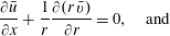 $$\begin{eqnarray}\displaystyle & \displaystyle \frac{\unicode[STIX]{x2202}\bar{u}}{\unicode[STIX]{x2202}x}+\frac{1}{r}\frac{\unicode[STIX]{x2202}(r\,\bar{v})}{\unicode[STIX]{x2202}r}=0,\quad \text{and} & \displaystyle\end{eqnarray}$$
 $$\begin{eqnarray}\displaystyle & \displaystyle \frac{\unicode[STIX]{x2202}\bar{u}}{\unicode[STIX]{x2202}t}+\bar{u}\frac{\unicode[STIX]{x2202}\bar{u}}{\unicode[STIX]{x2202}x}+\bar{v}\frac{\unicode[STIX]{x2202}\bar{u}}{\unicode[STIX]{x2202}r}=\unicode[STIX]{x1D708}\left(\frac{\unicode[STIX]{x2202}^{2}\bar{u}}{\unicode[STIX]{x2202}x^{2}}+\frac{\unicode[STIX]{x2202}^{2}\bar{u}}{\unicode[STIX]{x2202}r^{2}}\right)-\frac{\unicode[STIX]{x2202}\overline{u^{\prime }u^{\prime }}}{\unicode[STIX]{x2202}x}-\frac{1}{r}\frac{\unicode[STIX]{x2202}\left(r\,\overline{u^{\prime }v^{\prime }}\right)}{\unicode[STIX]{x2202}r}-\frac{1}{\unicode[STIX]{x1D70C}}\frac{\unicode[STIX]{x2202}\bar{p}}{\unicode[STIX]{x2202}x}, & \displaystyle\end{eqnarray}$$
where
 $u$
,
$u$
,
 $v$
,
$v$
,
 $\unicode[STIX]{x1D70C}$
and
$\unicode[STIX]{x1D70C}$
and
 $p$
are axial velocity, radial velocity, density and pressure, the overbar denotes circumferential and ensemble averaging, and prime denotes fluctuation from the mean. The velocity statistics, normalised by the centreline ensemble-averaged velocity (
$p$
are axial velocity, radial velocity, density and pressure, the overbar denotes circumferential and ensemble averaging, and prime denotes fluctuation from the mean. The velocity statistics, normalised by the centreline ensemble-averaged velocity (
 $\bar{u}_{c}(x,t)$
), are assumed to be self-similar with respect to a scaled radius
$\bar{u}_{c}(x,t)$
), are assumed to be self-similar with respect to a scaled radius
 $\unicode[STIX]{x1D702}=r/x$
. The averages appearing in (2.2) can then be expressed as
$\unicode[STIX]{x1D702}=r/x$
. The averages appearing in (2.2) can then be expressed as
 $$\begin{eqnarray}\displaystyle \bar{u}=\bar{u}_{c}f(\unicode[STIX]{x1D702}),\quad \bar{v}=\bar{u}_{c}g(\unicode[STIX]{x1D702}),\quad \overline{u^{\prime }v^{\prime }}=\bar{u}_{c}^{2}h(\unicode[STIX]{x1D702})\quad \text{and}\quad \overline{u^{\prime }u^{\prime }}+(\bar{p}-p_{0})/\unicode[STIX]{x1D70C}=\bar{u}_{c}^{2}k(\unicode[STIX]{x1D702}), & & \displaystyle\end{eqnarray}$$
where
 $f$
,
$f$
,
 $g$
,
$g$
,
 $h$
, and
$h$
, and
 $k$
are the shape functions of the corresponding flow properties, with
$k$
are the shape functions of the corresponding flow properties, with
 $p_{0}$
taken as the ambient pressure.
$p_{0}$
taken as the ambient pressure.
2.1 Centreline velocity evolution
Substituting the expressions for self-similar properties (2.3) into the continuity equation (2.1) and rearranging gives
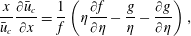 $$\begin{eqnarray}\displaystyle \frac{x}{\bar{u}_{c}}\frac{\unicode[STIX]{x2202}\bar{u}_{c}}{\unicode[STIX]{x2202}x}=\frac{1}{f}\left(\unicode[STIX]{x1D702}\frac{\unicode[STIX]{x2202}f}{\unicode[STIX]{x2202}\unicode[STIX]{x1D702}}-\frac{g}{\unicode[STIX]{x1D702}}-\frac{\unicode[STIX]{x2202}g}{\unicode[STIX]{x2202}\unicode[STIX]{x1D702}}\right), & & \displaystyle\end{eqnarray}$$
which is separably constant and leads to a solution for the centreline velocity
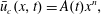 $$\begin{eqnarray}\displaystyle \bar{u}_{c}(x,t)=A(t)x^{n}, & & \displaystyle\end{eqnarray}$$
with time-dependent factor
 $A(t)$
. The exponent
$A(t)$
. The exponent
 $n$
will be constant within a self-similar region, but can vary between different self-similar regions. The momentum equation can be rearranged by substituting (2.3) and (2.5) into (2.2) and multiplying by
$n$
will be constant within a self-similar region, but can vary between different self-similar regions. The momentum equation can be rearranged by substituting (2.3) and (2.5) into (2.2) and multiplying by
 $x^{1-2n}/A^{2}$
, giving:
$x^{1-2n}/A^{2}$
, giving:
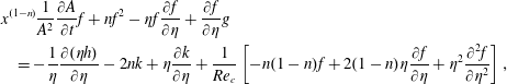 $$\begin{eqnarray}\displaystyle & & \displaystyle \displaystyle x^{(1-n)}\frac{1}{A^{2}}\frac{\unicode[STIX]{x2202}A}{\unicode[STIX]{x2202}t}f+nf^{2}-\unicode[STIX]{x1D702}f\frac{\unicode[STIX]{x2202}f}{\unicode[STIX]{x2202}\unicode[STIX]{x1D702}}+\frac{\unicode[STIX]{x2202}f}{\unicode[STIX]{x2202}\unicode[STIX]{x1D702}}g\nonumber\\ \displaystyle & & \displaystyle \quad \displaystyle =-\frac{1}{\unicode[STIX]{x1D702}}\frac{\unicode[STIX]{x2202}(\unicode[STIX]{x1D702}h)}{\unicode[STIX]{x2202}\unicode[STIX]{x1D702}}-2nk+\unicode[STIX]{x1D702}\frac{\unicode[STIX]{x2202}k}{\unicode[STIX]{x2202}\unicode[STIX]{x1D702}}+\frac{1}{Re_{c}}\left[-n(1-n)f+2(1-n)\unicode[STIX]{x1D702}\frac{\unicode[STIX]{x2202}f}{\unicode[STIX]{x2202}\unicode[STIX]{x1D702}}+\unicode[STIX]{x1D702}^{2}\frac{\unicode[STIX]{x2202}^{2}f}{\unicode[STIX]{x2202}\unicode[STIX]{x1D702}^{2}}\right],\qquad\end{eqnarray}$$
where
 $Re_{c}=\bar{u}_{c}x/\unicode[STIX]{x1D708}=Ax^{n+1}/\unicode[STIX]{x1D708}$
. Note that unlike statistically steady jets,
$Re_{c}=\bar{u}_{c}x/\unicode[STIX]{x1D708}=Ax^{n+1}/\unicode[STIX]{x1D708}$
. Note that unlike statistically steady jets,
 $Re_{c}$
can be time- and space-dependent for statistically unsteady jets. Henceforth,
$Re_{c}$
can be time- and space-dependent for statistically unsteady jets. Henceforth,
 $Re_{c}$
is assumed to be sufficiently large that the viscous terms can be neglected, but note that this assumption is not strictly applicable when the decelerating jet relaminarises. Self-similarity of (2.6) demands that
$Re_{c}$
is assumed to be sufficiently large that the viscous terms can be neglected, but note that this assumption is not strictly applicable when the decelerating jet relaminarises. Self-similarity of (2.6) demands that
 $n=1$
for the statistically unsteady jet. Solving (2.6) for
$n=1$
for the statistically unsteady jet. Solving (2.6) for
 $A(t)$
and substitution into (2.5) gives
$A(t)$
and substitution into (2.5) gives
 $$\begin{eqnarray}\displaystyle \bar{u}_{c}=\frac{x}{C_{A}(t-t_{0})}, & & \displaystyle\end{eqnarray}$$
where
 $C_{A}$
and
$C_{A}$
and
 $t_{0}$
are constants of integration, the latter of which is interpreted as the virtual time origin for the self-similar decelerating jet. Note that the first two viscous terms in (2.6) are then identically zero, and the Reynolds number,
$t_{0}$
are constants of integration, the latter of which is interpreted as the virtual time origin for the self-similar decelerating jet. Note that the first two viscous terms in (2.6) are then identically zero, and the Reynolds number,
 $Re_{c}$
, scales with
$Re_{c}$
, scales with
 $x^{2}$
and
$x^{2}$
and
 $t^{-1}$
. The dimensionless constant
$t^{-1}$
. The dimensionless constant
 $C_{A}$
is given by
$C_{A}$
is given by
 $$\begin{eqnarray}\displaystyle \underbrace{C_{A}f}_{-\unicode[STIX]{x2202}\bar{u}/\unicode[STIX]{x2202}t}=\underbrace{f^{2}-\unicode[STIX]{x1D702}f\frac{\unicode[STIX]{x2202}f}{\unicode[STIX]{x2202}\unicode[STIX]{x1D702}}}_{\bar{u}\unicode[STIX]{x2202}\bar{u}/\unicode[STIX]{x2202}x}+\underbrace{g\frac{\unicode[STIX]{x2202}f}{\unicode[STIX]{x2202}\unicode[STIX]{x1D702}}}_{\bar{v}\unicode[STIX]{x2202}\bar{u}/\unicode[STIX]{x2202}r}+\underbrace{\frac{1}{\unicode[STIX]{x1D702}}\frac{\unicode[STIX]{x2202}(\unicode[STIX]{x1D702}h)}{\unicode[STIX]{x2202}\unicode[STIX]{x1D702}}}_{\frac{1}{r}\frac{\unicode[STIX]{x2202}(r\overline{u^{\prime }v^{\prime }})}{\unicode[STIX]{x2202}r}}+\underbrace{2k-\unicode[STIX]{x1D702}\frac{\unicode[STIX]{x2202}k}{\unicode[STIX]{x2202}\unicode[STIX]{x1D702}}}_{\unicode[STIX]{x2202}(\overline{u^{\prime }u^{\prime }}+\overline{p/\unicode[STIX]{x1D70C}})/\unicode[STIX]{x2202}x}, & & \displaystyle\end{eqnarray}$$
where the origin of each term is labelled. If (2.8) is integrated over a cross-stream plane it becomes
 $$\begin{eqnarray}\displaystyle C_{A}=\frac{\displaystyle 4\int _{0}^{\infty }f^{2}\unicode[STIX]{x1D702}\,\text{d}\unicode[STIX]{x1D702}+4\int _{0}^{\infty }k\unicode[STIX]{x1D702}\,\text{d}\unicode[STIX]{x1D702}}{\displaystyle \int _{0}^{\infty }f\unicode[STIX]{x1D702}\,\text{d}\unicode[STIX]{x1D702}}. & & \displaystyle\end{eqnarray}$$
Since the integrals of
 $f$
and
$f$
and
 $f^{2}$
are necessarily positive and the magnitude of the integral of
$f^{2}$
are necessarily positive and the magnitude of the integral of
 $k$
is typically smaller than the integral of
$k$
is typically smaller than the integral of
 $f^{2}$
in a jet,
$f^{2}$
in a jet,
 $C_{A}$
is expected to be positive. Since positive
$C_{A}$
is expected to be positive. Since positive
 $C_{A}$
in (2.7) corresponds to deceleration, unsteady self-similarity in the form given by (2.3) is not expected in accelerating jets.
$C_{A}$
in (2.7) corresponds to deceleration, unsteady self-similarity in the form given by (2.3) is not expected in accelerating jets.
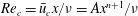
Figure 1. (a) Inverse centreline velocities measured at different downstream locations from pulsed jets of Witze (Reference Witze1983), with
 $X_{0}$
being the virtual origin and time measured from the start of the fluid injection pulse. (b) Cross-sectional colour maps of the instantaneous axial velocity at
$X_{0}$
being the virtual origin and time measured from the start of the fluid injection pulse. (b) Cross-sectional colour maps of the instantaneous axial velocity at
 $t/\unicode[STIX]{x1D70F}=1$
, 11 and 21 following stopping of the jet at
$t/\unicode[STIX]{x1D70F}=1$
, 11 and 21 following stopping of the jet at
 $t/\unicode[STIX]{x1D70F}=0$
, where
$t/\unicode[STIX]{x1D70F}=0$
, where
 $\unicode[STIX]{x1D70F}=D/U_{0}$
and time
$\unicode[STIX]{x1D70F}=D/U_{0}$
and time
 $t$
is measured from the start of the deceleration.
$t$
is measured from the start of the deceleration.
The measurements of Witze (Reference Witze1983) replotted in figure 1(a) exhibit a linear dependence between
 $(X-X_{0})/\bar{u}_{c}$
and time in the decelerating region of the jet, as predicted by (2.7), with
$(X-X_{0})/\bar{u}_{c}$
and time in the decelerating region of the jet, as predicted by (2.7), with
 $C_{A}=2.3$
providing the best fit to the data. The time values reported by Witze (Reference Witze1983) are measured from the start of the fluid injection pulse. The linear increase of axial mean velocity with axial distance in decelerating jets is in contrast with the observation in statistically steady jets that the centreline axial velocity is inversely proportional to axial distance (
$C_{A}=2.3$
providing the best fit to the data. The time values reported by Witze (Reference Witze1983) are measured from the start of the fluid injection pulse. The linear increase of axial mean velocity with axial distance in decelerating jets is in contrast with the observation in statistically steady jets that the centreline axial velocity is inversely proportional to axial distance (
 $n=-1$
). On the basis of their respectively different assumptions, Scase et al. (Reference Scase, Caulfield, Dalziel and Hunt2006), Craske & van Reeuwijk (Reference Craske and van Reeuwijk2015b
) and, in the limit
$n=-1$
). On the basis of their respectively different assumptions, Scase et al. (Reference Scase, Caulfield, Dalziel and Hunt2006), Craske & van Reeuwijk (Reference Craske and van Reeuwijk2015b
) and, in the limit
 $t\rightarrow \infty$
and
$t\rightarrow \infty$
and
 $x\rightarrow \infty$
, Musculus (Reference Musculus2009) also predict the
$x\rightarrow \infty$
, Musculus (Reference Musculus2009) also predict the
 $x/t$
dependence for the axial velocity scale in decelerating jets.
$x/t$
dependence for the axial velocity scale in decelerating jets.
Defining the location of the deceleration wave as the intersection of the centreline velocity profile of the original statistically steady jet and the centreline velocity predicted by (2.7) gives the speed of the deceleration wave equal to
 $$\begin{eqnarray}\displaystyle c_{wave}=\frac{C_{A}}{2}\,\overline{u}_{c,steady}. & & \displaystyle\end{eqnarray}$$
Based on
 $C_{A}/2\approx 1.1$
from the data of Witze (Reference Witze1983), the wave speed is approximately equal to the local centreline velocity in the initial statistically steady jet. A similar wave speed dependence arises in Musculus (Reference Musculus2009) where, considering an approximately Gaussian axial velocity profile, the constant of proportionality is equal to 1.0, and in Scase et al. (Reference Scase, Caulfield, Dalziel and Hunt2006) where, considering a top-hat velocity profile, small disturbances convect with the local speed of the jet.
$C_{A}/2\approx 1.1$
from the data of Witze (Reference Witze1983), the wave speed is approximately equal to the local centreline velocity in the initial statistically steady jet. A similar wave speed dependence arises in Musculus (Reference Musculus2009) where, considering an approximately Gaussian axial velocity profile, the constant of proportionality is equal to 1.0, and in Scase et al. (Reference Scase, Caulfield, Dalziel and Hunt2006) where, considering a top-hat velocity profile, small disturbances convect with the local speed of the jet.
2.2 Radial velocity profiles
The shape function for the mean radial velocity
 $g$
in a decelerating self-similar jet can be expressed in terms of the axial velocity shape function
$g$
in a decelerating self-similar jet can be expressed in terms of the axial velocity shape function
 $f$
by integrating the continuity equation (2.4),
$f$
by integrating the continuity equation (2.4),
 $$\begin{eqnarray}\displaystyle g=\unicode[STIX]{x1D702}f-\frac{n+2}{\unicode[STIX]{x1D702}}\int _{0}^{\unicode[STIX]{x1D702}}\unicode[STIX]{x1D702}^{\prime }f\,\text{d}\unicode[STIX]{x1D702}^{\prime }. & & \displaystyle\end{eqnarray}$$
The relationship between
 $f$
and
$f$
and
 $g$
therefore depends on whether the self-similar jet is statistically steady (
$g$
therefore depends on whether the self-similar jet is statistically steady (
 $n=-1$
) or decelerating (
$n=-1$
) or decelerating (
 $n=1$
). Differentiating (2.11) with respect to
$n=1$
). Differentiating (2.11) with respect to
 $\unicode[STIX]{x1D702}$
and considering the rotational symmetry of the flow implies that
$\unicode[STIX]{x1D702}$
and considering the rotational symmetry of the flow implies that
 $\unicode[STIX]{x2202}g/\unicode[STIX]{x2202}\unicode[STIX]{x1D702}=-n/2$
at the centreline. It is well known that
$\unicode[STIX]{x2202}g/\unicode[STIX]{x2202}\unicode[STIX]{x1D702}=-n/2$
at the centreline. It is well known that
 $\unicode[STIX]{x2202}g/\unicode[STIX]{x2202}\unicode[STIX]{x1D702}=0.5$
at the centreline of a statistically steady round turbulent jet (e.g. Pope Reference Pope2000), and this value is recovered with
$\unicode[STIX]{x2202}g/\unicode[STIX]{x2202}\unicode[STIX]{x1D702}=0.5$
at the centreline of a statistically steady round turbulent jet (e.g. Pope Reference Pope2000), and this value is recovered with
 $n=-1$
. The corresponding prediction for a decelerating self-similar jet with
$n=-1$
. The corresponding prediction for a decelerating self-similar jet with
 $n=1$
is that
$n=1$
is that
 $\unicode[STIX]{x2202}g/\unicode[STIX]{x2202}\unicode[STIX]{x1D702}=-0.5$
, indicating that the radial velocity reverses near to the centreline in the deceleration wave.
$\unicode[STIX]{x2202}g/\unicode[STIX]{x2202}\unicode[STIX]{x1D702}=-0.5$
, indicating that the radial velocity reverses near to the centreline in the deceleration wave.
The different radial velocity profile in the statistically unsteady jet changes the rate of mass entrainment,
 $E=-2\unicode[STIX]{x03C0}\unicode[STIX]{x1D70C}x\bar{u}_{c}\lim _{\unicode[STIX]{x1D702}\rightarrow \infty }(\unicode[STIX]{x1D702}g)$
. Using (2.11), the normalised entrainment rate for the self-similar jet can be written
$E=-2\unicode[STIX]{x03C0}\unicode[STIX]{x1D70C}x\bar{u}_{c}\lim _{\unicode[STIX]{x1D702}\rightarrow \infty }(\unicode[STIX]{x1D702}g)$
. Using (2.11), the normalised entrainment rate for the self-similar jet can be written
 $$\begin{eqnarray}\displaystyle \frac{E}{\unicode[STIX]{x1D70C}x\bar{u}_{c}}=\lim _{\unicode[STIX]{x1D702}\rightarrow \infty }\left[-2\unicode[STIX]{x03C0}\unicode[STIX]{x1D702}^{2}f+(n+2)\int _{0}^{\unicode[STIX]{x1D702}}2\unicode[STIX]{x03C0}\unicode[STIX]{x1D702}^{\prime }f\,\text{d}\unicode[STIX]{x1D702}^{\prime }\right]=(n+2)Q_{\unicode[STIX]{x1D702}}, & & \displaystyle\end{eqnarray}$$
with integral mass flux
 $Q_{\unicode[STIX]{x1D702}}=\int _{0}^{\infty }2\unicode[STIX]{x03C0}\unicode[STIX]{x1D702}f\,\text{d}\unicode[STIX]{x1D702}$
. If the integrated mass flux
$Q_{\unicode[STIX]{x1D702}}=\int _{0}^{\infty }2\unicode[STIX]{x03C0}\unicode[STIX]{x1D702}f\,\text{d}\unicode[STIX]{x1D702}$
. If the integrated mass flux
 $Q_{\unicode[STIX]{x1D702}}$
remains constant, as assumed by Musculus (Reference Musculus2009), the scaled mass entrainment rate in the decelerating self-similar jet (
$Q_{\unicode[STIX]{x1D702}}$
remains constant, as assumed by Musculus (Reference Musculus2009), the scaled mass entrainment rate in the decelerating self-similar jet (
 $n=1$
) is predicted to be three times the rate in a statistically stationary jet (
$n=1$
) is predicted to be three times the rate in a statistically stationary jet (
 $n=-1$
). However, the mean axial velocity profile and therefore the integrated mass flux
$n=-1$
). However, the mean axial velocity profile and therefore the integrated mass flux
 $Q_{\unicode[STIX]{x1D702}}$
are also subject to change within the decelerating region of the jet (Borée et al.
Reference Borée, Atassi and Charnay1996), further affecting the scaled entrainment rate given by (2.12). To be shown in (2.14), the unsteady self-similar
$Q_{\unicode[STIX]{x1D702}}$
are also subject to change within the decelerating region of the jet (Borée et al.
Reference Borée, Atassi and Charnay1996), further affecting the scaled entrainment rate given by (2.12). To be shown in (2.14), the unsteady self-similar
 $h$
-profile depends on the corresponding
$h$
-profile depends on the corresponding
 $f$
-profile, indicating that
$f$
-profile, indicating that
 $Q_{\unicode[STIX]{x1D702}}$
and
$Q_{\unicode[STIX]{x1D702}}$
and
 $h$
are not independent each other.
$h$
are not independent each other.
2.3 Reynolds shear stress profiles
An expression for the shape function
 $h$
for the Reynolds shear stress
$h$
for the Reynolds shear stress
 $\overline{u^{\prime }v^{\prime }}$
in self-similar jets can be obtained from (2.6). For a statistically steady jet with
$\overline{u^{\prime }v^{\prime }}$
in self-similar jets can be obtained from (2.6). For a statistically steady jet with
 $n=-1$
,
$n=-1$
,
 $$\begin{eqnarray}\displaystyle h=\frac{f}{\unicode[STIX]{x1D702}}\int _{0}^{\unicode[STIX]{x1D702}}\unicode[STIX]{x1D702}^{\prime }f\,\text{d}\unicode[STIX]{x1D702}^{\prime }+\unicode[STIX]{x1D702}k. & & \displaystyle\end{eqnarray}$$
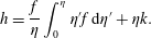
At the centreline, the gradient of
 $h$
is
$h$
is
 $\unicode[STIX]{x2202}h/\unicode[STIX]{x2202}\unicode[STIX]{x1D702}=1/2+k(0)$
. The typical centreline value of shape function
$\unicode[STIX]{x2202}h/\unicode[STIX]{x2202}\unicode[STIX]{x1D702}=1/2+k(0)$
. The typical centreline value of shape function
 $k$
in a statistically steady jet is approximately 0.025 (e.g. Pope Reference Pope2000) which, with
$k$
in a statistically steady jet is approximately 0.025 (e.g. Pope Reference Pope2000) which, with
 $n=-1$
, gives
$n=-1$
, gives
 $(\unicode[STIX]{x2202}h/\unicode[STIX]{x2202}\unicode[STIX]{x1D702})_{\unicode[STIX]{x1D702}=0}\approx 0.525$
.
$(\unicode[STIX]{x2202}h/\unicode[STIX]{x2202}\unicode[STIX]{x1D702})_{\unicode[STIX]{x1D702}=0}\approx 0.525$
.
For a self-similar decelerating jet, using (2.7) and
 $n=1$
in (2.6) gives,
$n=1$
in (2.6) gives,
 $$\begin{eqnarray}\displaystyle h=\frac{C_{A}}{\unicode[STIX]{x1D702}}\int _{0}^{\unicode[STIX]{x1D702}}\unicode[STIX]{x1D702}^{\prime }f\,\text{d}\unicode[STIX]{x1D702}^{\prime }+\frac{4}{\unicode[STIX]{x1D702}}\int _{0}^{\unicode[STIX]{x1D702}}\unicode[STIX]{x1D702}^{\prime }f^{2}\,\text{d}\unicode[STIX]{x1D702}^{\prime }+\frac{3f}{\unicode[STIX]{x1D702}}\int _{0}^{\unicode[STIX]{x1D702}}\unicode[STIX]{x1D702}^{\prime }f\,\text{d}\unicode[STIX]{x1D702}^{\prime }+\unicode[STIX]{x1D702}k-\frac{4}{\unicode[STIX]{x1D702}}\int _{0}^{\unicode[STIX]{x1D702}}\unicode[STIX]{x1D702}^{\prime }k\,\text{d}\unicode[STIX]{x1D702}^{\prime }. & & \displaystyle\end{eqnarray}$$
Differentiating the expression for
 $h$
with respect to
$h$
with respect to
 $\unicode[STIX]{x1D702}$
and evaluating it at
$\unicode[STIX]{x1D702}$
and evaluating it at
 $\unicode[STIX]{x1D702}=0$
gives
$\unicode[STIX]{x1D702}=0$
gives
 $\unicode[STIX]{x2202}h/\unicode[STIX]{x2202}\unicode[STIX]{x1D702}=(C_{A}-1)/2+k(0)$
, which provides a convenient means for evaluating
$\unicode[STIX]{x2202}h/\unicode[STIX]{x2202}\unicode[STIX]{x1D702}=(C_{A}-1)/2+k(0)$
, which provides a convenient means for evaluating
 $C_{A}$
from the
$C_{A}$
from the
 $h$
gradient and
$h$
gradient and
 $k$
at the centreline.
$k$
at the centreline.
3 Simulation details
The data presented were obtained from DNS of a stopping jet. The simulation methods and an analysis of the precursor statistically steady turbulent jet solution were reported in Shin, Sandberg & Richardson (Reference Shin, Sandberg and Richardson2017). Initially, a round jet with jet Reynolds number
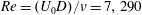 $Re=(U_{0}D)/\unicode[STIX]{x1D708}=7,290$
was issued from a flat plate into a quiescent environment, where
$Re=(U_{0}D)/\unicode[STIX]{x1D708}=7,290$
was issued from a flat plate into a quiescent environment, where
 $U_{0}$
was the bulk jet velocity,
$U_{0}$
was the bulk jet velocity,
 $D$
was the jet inlet diameter, and
$D$
was the jet inlet diameter, and
 $\unicode[STIX]{x1D708}$
was the kinematic viscosity. Pseudo-turbulent velocity fluctuations with 1.7 % turbulence intensity were superimposed on an approximately top-hat velocity profile. Shin et al. (Reference Shin, Sandberg and Richardson2017) showed that the velocity field in the precursor statistically steady jet simulation was statistically stationary and displayed self-similarity downstream of an initial development region. The centreline decay rate constant was 6.7, consistent with experimental data of Weisgraber & Liepmann (Reference Weisgraber and Liepmann1998). The mean axial and radial velocities and the Reynolds shear stress were found to be in agreement with laboratory measurements from a converging jet nozzle by Panchapakesan & Lumley (Reference Panchapakesan and Lumley1993). Shin et al. (Reference Shin, Sandberg and Richardson2017) also demonstrated self-similarity of jet fluid mass fraction statistics in agreement with measurement data from a converging nozzle experiment by Mi, Nathan & Nobes (Reference Mi, Nathan and Nobes2001).
$\unicode[STIX]{x1D708}$
was the kinematic viscosity. Pseudo-turbulent velocity fluctuations with 1.7 % turbulence intensity were superimposed on an approximately top-hat velocity profile. Shin et al. (Reference Shin, Sandberg and Richardson2017) showed that the velocity field in the precursor statistically steady jet simulation was statistically stationary and displayed self-similarity downstream of an initial development region. The centreline decay rate constant was 6.7, consistent with experimental data of Weisgraber & Liepmann (Reference Weisgraber and Liepmann1998). The mean axial and radial velocities and the Reynolds shear stress were found to be in agreement with laboratory measurements from a converging jet nozzle by Panchapakesan & Lumley (Reference Panchapakesan and Lumley1993). Shin et al. (Reference Shin, Sandberg and Richardson2017) also demonstrated self-similarity of jet fluid mass fraction statistics in agreement with measurement data from a converging nozzle experiment by Mi, Nathan & Nobes (Reference Mi, Nathan and Nobes2001).
The present decelerating jet simulations were run by restarting a precursor simulation from Shin et al. (Reference Shin, Sandberg and Richardson2017) and abruptly reducing the inflow velocity at a start time taken as
 $t=0$
. The evolution of the axial velocity field after the inflow was stopped is shown in figure 1(b). Four statistically independent realisations of the stopping event were simulated to provide statistics for the deceleration process.
$t=0$
. The evolution of the axial velocity field after the inflow was stopped is shown in figure 1(b). Four statistically independent realisations of the stopping event were simulated to provide statistics for the deceleration process.
The simulations were performed with the HiPSTAR DNS code (Sandberg & Tester Reference Sandberg and Tester2016), solving the compressible Navier–Stokes equations in a cylindrical coordinate system. The numerical approach is described fully by Shin et al. (Reference Shin, Sandberg and Richardson2017). The Kolmogorov length scales in the flow are expected to increase during the deceleration transient since the jet width remains approximately constant (Craske & van Reeuwijk Reference Craske and van Reeuwijk2015b
) while velocity magnitudes decrease. Therefore the numerical grid used for the precursor statistically steady jet simulation (Shin et al.
Reference Shin, Sandberg and Richardson2017) provides sufficient resolution for the decelerating jet simulation, and the same grid was retained for this study. The grid consisted of
 $3020\times 834\times 130$
structured nodes in the axial, radial and circumferential directions (
$3020\times 834\times 130$
structured nodes in the axial, radial and circumferential directions (
 ${\approx}327$
million nodes in total), spanning axially from
${\approx}327$
million nodes in total), spanning axially from
 $x/D=0{-}60$
and radially from
$x/D=0{-}60$
and radially from
 $r/D=0{-}30$
. The grid was stretched to provide greater refinement in the shear layer near to the jet inlet, with 145 points radially across the diameter of the jet.
$r/D=0{-}30$
. The grid was stretched to provide greater refinement in the shear layer near to the jet inlet, with 145 points radially across the diameter of the jet.
4 Results
4.1 Centreline velocity evolution
Here, the DNS data are used to investigate how the centreline profile of the mean axial velocity varies in the stopping jet, and to assess the validity of (2.7). Statistical properties of the flow are evaluated at each instant by averaging in the circumferential direction, due to the statistical rotational symmetry of the flow, and ensemble averaging of the four realisations of the simulation. Figure 2(a) shows ensemble-averaged profiles of axial velocity along the centreline, where the virtual origin is taken as
 $2.3D$
downstream of the inlet, as in the analysis of the statistically steady jet (Shin et al.
Reference Shin, Sandberg and Richardson2017). For reference, the averaged axial velocity from the initial statistically steady jet is shown as a thick solid line. Once the jet inflow is arrested, a deceleration wave travels downstream at a speed close to the local centreline velocity. Upstream of the deceleration wave, the centreline axial velocity decays over time and develops a linear dependence on
$2.3D$
downstream of the inlet, as in the analysis of the statistically steady jet (Shin et al.
Reference Shin, Sandberg and Richardson2017). For reference, the averaged axial velocity from the initial statistically steady jet is shown as a thick solid line. Once the jet inflow is arrested, a deceleration wave travels downstream at a speed close to the local centreline velocity. Upstream of the deceleration wave, the centreline axial velocity decays over time and develops a linear dependence on
 $x$
, with the gradient decreasing in time. Downstream of the deceleration wave, the centreline velocity profile is yet to be affected by the deceleration and resembles the profile of the statistically steady jet.
$x$
, with the gradient decreasing in time. Downstream of the deceleration wave, the centreline velocity profile is yet to be affected by the deceleration and resembles the profile of the statistically steady jet.
Figure 2(b) shows that, taking
 $t_{0}=14\unicode[STIX]{x1D70F}$
with
$t_{0}=14\unicode[STIX]{x1D70F}$
with
 $\unicode[STIX]{x1D70F}=D/U_{0}$
, the quantity
$\unicode[STIX]{x1D70F}=D/U_{0}$
, the quantity
 $\bar{u}_{c}(t-t_{0})/x$
asymptotes towards the value
$\bar{u}_{c}(t-t_{0})/x$
asymptotes towards the value
 $1/C_{A}=0.46$
. The resulting value
$1/C_{A}=0.46$
. The resulting value
 $C_{A}=2.2$
in the stopping jet simulation is close to the value
$C_{A}=2.2$
in the stopping jet simulation is close to the value
 $C_{A}=2.3$
obtained from the data from Witze (Reference Witze1983) in figure 1(a). The time taken for the asymptotic decelerating state to arrive at
$C_{A}=2.3$
obtained from the data from Witze (Reference Witze1983) in figure 1(a). The time taken for the asymptotic decelerating state to arrive at
 $x=18D$
is approximately
$x=18D$
is approximately
 $40\unicode[STIX]{x1D70F}$
. The value
$40\unicode[STIX]{x1D70F}$
. The value
 $t_{0}=14\unicode[STIX]{x1D70F}$
is obtained by fitting (2.7) to data from the decelerating region of the near-field (
$t_{0}=14\unicode[STIX]{x1D70F}$
is obtained by fitting (2.7) to data from the decelerating region of the near-field (
 $0<x/D<20$
) after reaching the asymptotic decelerating state (
$0<x/D<20$
) after reaching the asymptotic decelerating state (
 $t>40\unicode[STIX]{x1D70F}$
). The agreement between (2.7) and data from the decelerating region of the jet demonstrates that the dynamics of the centreline mean axial velocity are consistent with the assumption of self-similarity used to derive (2.7).
$t>40\unicode[STIX]{x1D70F}$
). The agreement between (2.7) and data from the decelerating region of the jet demonstrates that the dynamics of the centreline mean axial velocity are consistent with the assumption of self-similarity used to derive (2.7).
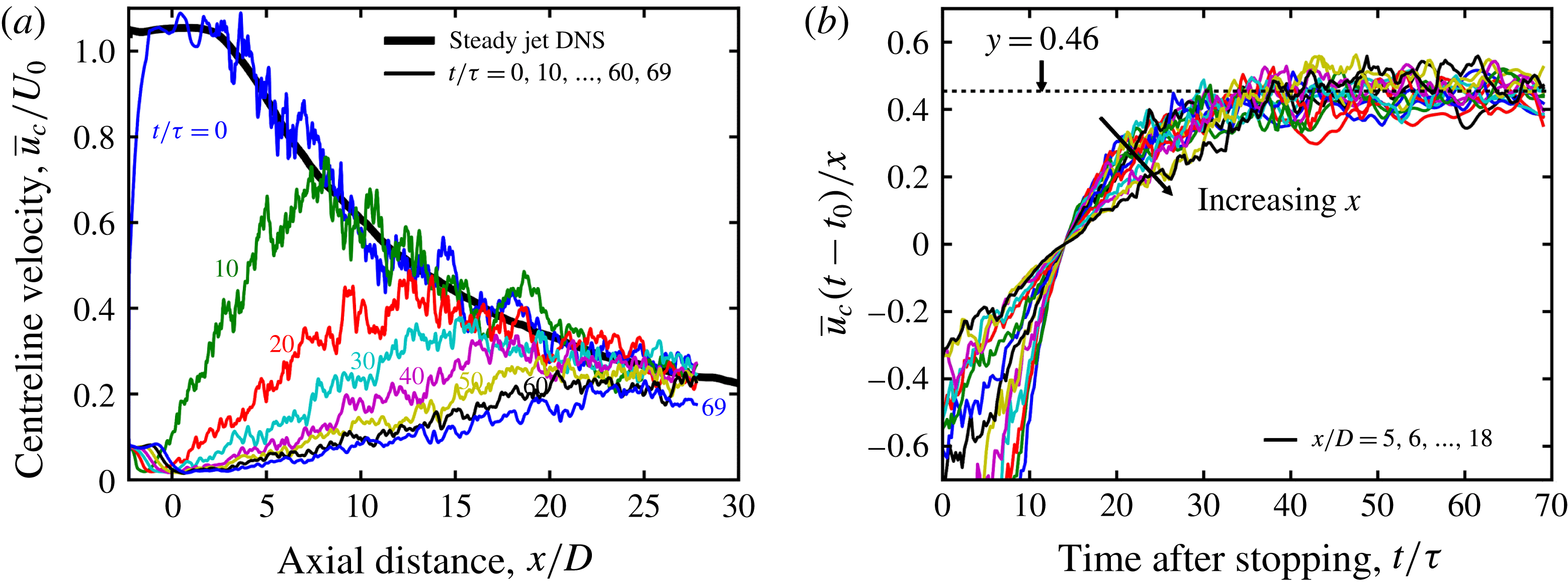
Figure 2. (a) Centreline profiles of the mean axial velocity at several instants in the range
 $t/\unicode[STIX]{x1D70F}=0{-}69$
. A supplementary animation of the temporal evolution of the profile is available online at https://doi.org/10.1017/jfm.2017.600 (movie 1). (b) The temporal evolution of the centreline mean axial velocity at several axial positions in the range
$t/\unicode[STIX]{x1D70F}=0{-}69$
. A supplementary animation of the temporal evolution of the profile is available online at https://doi.org/10.1017/jfm.2017.600 (movie 1). (b) The temporal evolution of the centreline mean axial velocity at several axial positions in the range
 $x/D=5{-}18$
.
$x/D=5{-}18$
.
4.2 Self-similar profiles
The analysis developed in § 2 relies upon the radial profiles of normalised velocity statistics being self-similar. Figure 3 compares the radial profiles of
 $\bar{u}$
,
$\bar{u}$
,
 $\bar{v}$
,
$\bar{v}$
,
 $\overline{u^{\prime }v^{\prime }}$
,
$\overline{u^{\prime }v^{\prime }}$
,
 $\overline{u^{\prime }u^{\prime }}$
,
$\overline{u^{\prime }u^{\prime }}$
,
 $\overline{v^{\prime }v^{\prime }}$
, and
$\overline{v^{\prime }v^{\prime }}$
, and
 $\overline{(p-p_{0})/\unicode[STIX]{x1D70C}}$
from the decelerating region of the stopping jet averaged over
$\overline{(p-p_{0})/\unicode[STIX]{x1D70C}}$
from the decelerating region of the stopping jet averaged over
 $50<t/\unicode[STIX]{x1D70F}<69$
and
$50<t/\unicode[STIX]{x1D70F}<69$
and
 $10<x/D<18$
and from the same spatial region of the initial statistically steady jet. Additional lines corresponding to predictions from § 2 are also shown for comparison. To reduce the influence of fluctuations of the centreline mean axial velocity caused by the limited statistical convergence in the data, the velocity statistics from the decelerating jet are normalised by a smoothed centreline mean axial velocity obtained by fitting a sixth-order polynomial to the data. The shaded region in each panel of figure 3 covers one standard deviation either side of the average profile from the decelerating jet. This deviation is due to finite statistical convergence of the instantaneous ensemble-averaged shape functions in the data, and due to any continuing development of the instantaneous ensemble-averaged profiles through the axial and temporal averaging windows. The magnitude of the deviation is sufficiently small that the data show a clear distinction between the profiles in the statistically steady jet and a new asymptotic self-similar state reached in the decelerating region of the stopping jet. For reference purposes, ensemble-averaged profiles showing the transition between the initial statistically steady state and the asymptotic decelerating self-similar state shown in figure 3 are provided as supplementary movies 2–7 and figure 1 in the supplementary material, for a selection of time instants and axial positions.
$10<x/D<18$
and from the same spatial region of the initial statistically steady jet. Additional lines corresponding to predictions from § 2 are also shown for comparison. To reduce the influence of fluctuations of the centreline mean axial velocity caused by the limited statistical convergence in the data, the velocity statistics from the decelerating jet are normalised by a smoothed centreline mean axial velocity obtained by fitting a sixth-order polynomial to the data. The shaded region in each panel of figure 3 covers one standard deviation either side of the average profile from the decelerating jet. This deviation is due to finite statistical convergence of the instantaneous ensemble-averaged shape functions in the data, and due to any continuing development of the instantaneous ensemble-averaged profiles through the axial and temporal averaging windows. The magnitude of the deviation is sufficiently small that the data show a clear distinction between the profiles in the statistically steady jet and a new asymptotic self-similar state reached in the decelerating region of the stopping jet. For reference purposes, ensemble-averaged profiles showing the transition between the initial statistically steady state and the asymptotic decelerating self-similar state shown in figure 3 are provided as supplementary movies 2–7 and figure 1 in the supplementary material, for a selection of time instants and axial positions.

Figure 3. Self-similar profiles averaged over
 $x/D=12.5-20$
and
$x/D=12.5-20$
and
 $t/\unicode[STIX]{x1D70F}=50-69$
of (a) axial velocity, (b) radial velocity, (c)
$t/\unicode[STIX]{x1D70F}=50-69$
of (a) axial velocity, (b) radial velocity, (c)
 $\overline{u^{\prime }v^{\prime }}$
, (d)
$\overline{u^{\prime }v^{\prime }}$
, (d)
 $\overline{u^{\prime }u^{\prime }}$
, (e)
$\overline{u^{\prime }u^{\prime }}$
, (e)
 $\overline{v^{\prime }v^{\prime }}$
, and (f) pressure.
$\overline{v^{\prime }v^{\prime }}$
, and (f) pressure.
Figure 3(a) shows that the mean axial velocity profile in the stopping jet transitions from the near-Gaussian steady-state profile to a slightly fuller profile in the decelerating region, similar to the change of shape recorded by Borée et al. (Reference Borée, Atassi and Charnay1996) in the statistically unsteady region after halving the jet flow rate. The overall width of the profile remains unchanged, supporting the assumption of a constant jet spreading angle used in the model by Musculus (Reference Musculus2009).
Figure 3(b) shows that there is a marked difference between mean radial velocity profiles in the deceleration region and in the statistically steady jet. As predicted in § 2.2, the centreline gradient of the mean radial velocity is very close to the value of
 $-0.5$
, and so opposite to the value in the statistically steady jet. The overall radial velocity profile in the decelerating region is in approximate agreement with (2.11) evaluated using the axial velocity profiles from figure 3(a) for either the statistically steady or stopping jets. The normalised radial velocity magnitude at
$-0.5$
, and so opposite to the value in the statistically steady jet. The overall radial velocity profile in the decelerating region is in approximate agreement with (2.11) evaluated using the axial velocity profiles from figure 3(a) for either the statistically steady or stopping jets. The normalised radial velocity magnitude at
 $\unicode[STIX]{x1D702}\rightarrow \infty$
increases by a factor of 3.6 during the deceleration transient. The dominant contribution to the increase in entrainment rate is the factor of three change of the factor (
$\unicode[STIX]{x1D702}\rightarrow \infty$
increases by a factor of 3.6 during the deceleration transient. The dominant contribution to the increase in entrainment rate is the factor of three change of the factor (
 $2+n$
) in (2.12), which derives from self-similarity and incompressibility of the fluid. The remaining 20 % contribution is likely due to the integrated mass flux
$2+n$
) in (2.12), which derives from self-similarity and incompressibility of the fluid. The remaining 20 % contribution is likely due to the integrated mass flux
 $Q_{\unicode[STIX]{x1D702}}$
increasing due to the change in the mean axial velocity profile shown in figure 3(a). The actual calculated increase of
$Q_{\unicode[STIX]{x1D702}}$
increasing due to the change in the mean axial velocity profile shown in figure 3(a). The actual calculated increase of
 $Q_{\unicode[STIX]{x1D702}}$
from figure 3(a) is about 30 % when integrated over
$Q_{\unicode[STIX]{x1D702}}$
from figure 3(a) is about 30 % when integrated over
 $\unicode[STIX]{x1D702}\in [0,0.23]$
. Considering the statistical convergence error on the axial and radial velocities, the increased
$\unicode[STIX]{x1D702}\in [0,0.23]$
. Considering the statistical convergence error on the axial and radial velocities, the increased
 $Q_{\unicode[STIX]{x1D702}}$
is in close agreement with the remaining 20 % increase of the entrainment rate.
$Q_{\unicode[STIX]{x1D702}}$
is in close agreement with the remaining 20 % increase of the entrainment rate.
Figure 3(c–e) shows that the peak magnitudes of the Reynolds stresses approximately double upstream of the deceleration wave. The overall profile of
 $h$
is well modelled by (2.14), using
$h$
is well modelled by (2.14), using
 $f$
and
$f$
and
 $k$
profiles from the self-similar decelerating region of the stopping jet, with the centreline gradient of
$k$
profiles from the self-similar decelerating region of the stopping jet, with the centreline gradient of
 $h$
in close agreement with the prediction given by
$h$
in close agreement with the prediction given by
 $(C_{A}-1)/2+k(0)\approx 0.6$
. Neglecting the terms in (2.14) involving
$(C_{A}-1)/2+k(0)\approx 0.6$
. Neglecting the terms in (2.14) involving
 $k$
has a minor impact on the overall prediction of
$k$
has a minor impact on the overall prediction of
 $h$
, implying that the Reynolds shear stress profile can be estimated based only on the axial velocity profile
$h$
, implying that the Reynolds shear stress profile can be estimated based only on the axial velocity profile
 $f$
, which itself is approximated reasonably closely by the self-similar profile of the initial statistically steady jet. A more comprehensive examination of the turbulent transport budgets could be considered in future work.
$f$
, which itself is approximated reasonably closely by the self-similar profile of the initial statistically steady jet. A more comprehensive examination of the turbulent transport budgets could be considered in future work.
Figure 3(f) shows the self-similar profiles of the pressure term
 $\overline{(p-p_{0})/\unicode[STIX]{x1D70C}}$
, with the profile of
$\overline{(p-p_{0})/\unicode[STIX]{x1D70C}}$
, with the profile of
 $-\overline{v^{\prime }v^{\prime }}$
from the decelerating jet added for reference. Analysis of statistically steady jets shows that there is an approximate balance between
$-\overline{v^{\prime }v^{\prime }}$
from the decelerating jet added for reference. Analysis of statistically steady jets shows that there is an approximate balance between
 $\overline{v^{\prime }v^{\prime }}$
and the pressure term (e.g. Pope Reference Pope2000). However, the peak magnitude of
$\overline{v^{\prime }v^{\prime }}$
and the pressure term (e.g. Pope Reference Pope2000). However, the peak magnitude of
 $\overline{v^{\prime }v^{\prime }}$
in the deceleration region of the jet is double the peak magnitude of the pressure term, and this imbalance provides a measure of the acceleration of fluid towards the centreline of the decelerating jet.
$\overline{v^{\prime }v^{\prime }}$
in the deceleration region of the jet is double the peak magnitude of the pressure term, and this imbalance provides a measure of the acceleration of fluid towards the centreline of the decelerating jet.
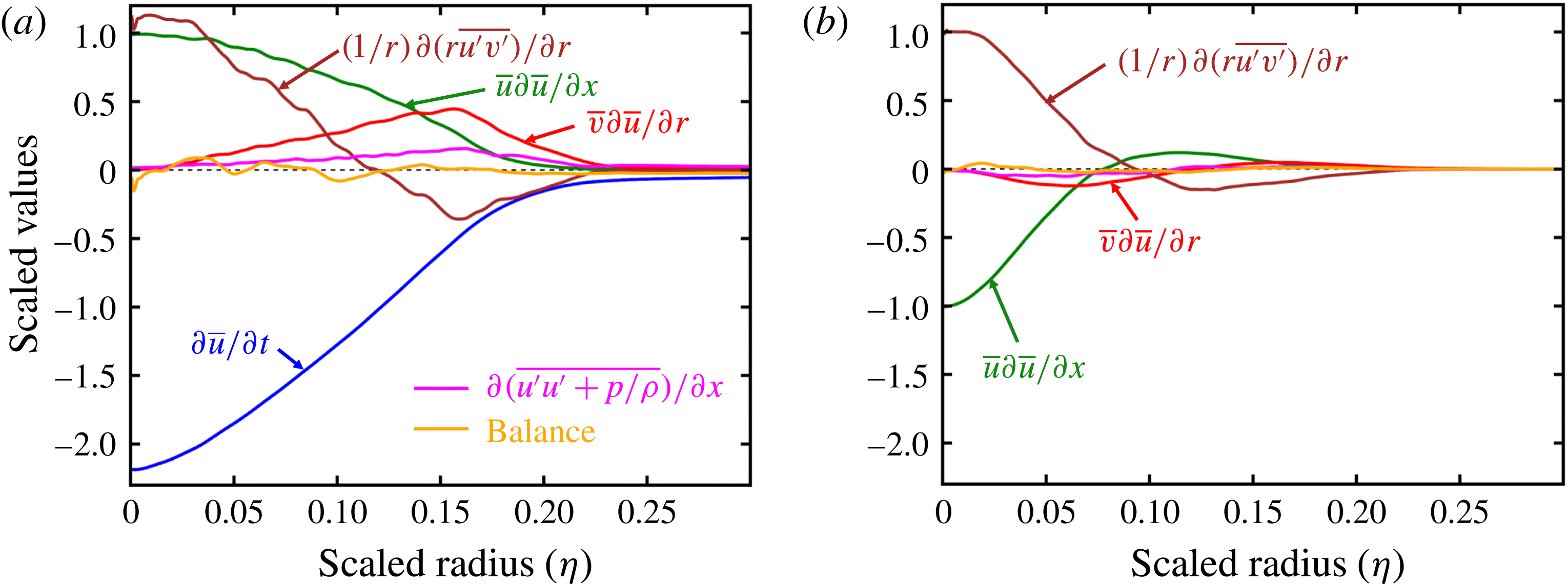
Figure 4. Budget terms of
 $x$
-momentum equation for (a) the decelerating region of the stopping jet and (b) the statistically steady jet.
$x$
-momentum equation for (a) the decelerating region of the stopping jet and (b) the statistically steady jet.
4.3 Momentum budgets
Figure 4 presents the budget of the momentum equation for self-similar round jets (2.6) evaluated using profiles of
 $f$
,
$f$
,
 $g$
,
$g$
,
 $h$
and
$h$
and
 $k$
from figure 3(a–f), both for the statistically steady jet and for the decelerating region of the stopping jet. The budget is scaled to give
$k$
from figure 3(a–f), both for the statistically steady jet and for the decelerating region of the stopping jet. The budget is scaled to give
 $\bar{u}\unicode[STIX]{x2202}\bar{u}/\unicode[STIX]{x2202}x=-1$
and 1 at the centreline in the statistically steady and stopping jets, respectively. Comparison with the statistically steady jet momentum budget shows that the deceleration (
$\bar{u}\unicode[STIX]{x2202}\bar{u}/\unicode[STIX]{x2202}x=-1$
and 1 at the centreline in the statistically steady and stopping jets, respectively. Comparison with the statistically steady jet momentum budget shows that the deceleration (
 $\unicode[STIX]{x2202}\bar{u}/\unicode[STIX]{x2202}t$
) in the stopping jet is dominated by the influx of lower-momentum fluid due to axial convection (
$\unicode[STIX]{x2202}\bar{u}/\unicode[STIX]{x2202}t$
) in the stopping jet is dominated by the influx of lower-momentum fluid due to axial convection (
 $\bar{u}\unicode[STIX]{x2202}\bar{u}/\unicode[STIX]{x2202}x$
) and radial entrainment (
$\bar{u}\unicode[STIX]{x2202}\bar{u}/\unicode[STIX]{x2202}x$
) and radial entrainment (
 $\bar{v}\unicode[STIX]{x2202}\bar{u}/\unicode[STIX]{x2202}r$
), with enhanced engulfment of low-momentum fluid indicated by greater area under the Reynolds shear stress term (
$\bar{v}\unicode[STIX]{x2202}\bar{u}/\unicode[STIX]{x2202}r$
), with enhanced engulfment of low-momentum fluid indicated by greater area under the Reynolds shear stress term (
 $(1/r)\unicode[STIX]{x2202}(r\overline{u^{\prime }v^{\prime }})/\unicode[STIX]{x2202}r$
). The small magnitude of the balance term confirms that the viscous terms omitted from (2.6) are negligibly small for the period considered.
$(1/r)\unicode[STIX]{x2202}(r\overline{u^{\prime }v^{\prime }})/\unicode[STIX]{x2202}r$
). The small magnitude of the balance term confirms that the viscous terms omitted from (2.6) are negligibly small for the period considered.
5 Conclusion
The decelerating flow in a stopping turbulent round jet is investigated using DNS. Upon stopping the inflow, a deceleration wave travels through the initially statistically steady turbulent jet. It is found that normalised velocity moments appearing in the unsteady momentum equation evolve towards a statistically stationary and axially uniform self-similar state in the decelerating region of the flow. Self-similarity leads to analytical relations concerning the evolution of the centreline mean axial velocity and the shapes of the radial profiles of the velocity statistics. The predictions derived from the assumption of self-similarity are shown to be consistent with data from the stopping jet. In particular, the centreline mean axial velocity is predicted to be proportional to axial position and inversely proportional to time upstream of the deceleration wave, with the wave speed proportional to the local centreline velocity in the preceding statistically steady turbulent jet. Furthermore, the mean radial velocity is predicted to reverse in direction near to the jet centreline as the deceleration wave passes, contributing to an approximately threefold increase in the normalised mass entrainment rate. The shape of the mean axial velocity profile undergoes a relatively small change across the deceleration transient; however, this change contributes 20 % of the enhancement of the mass entrainment rate. Previous modelling for unsteady jets based on the assumption that the shape of the mean axial velocity profile remains unchanged may benefit by taking account of the new decelerating self-similar state observed in this study.
Acknowledgements
This work has been performed with support from the EPSRC EP/L002698/1, EP/M001482/1, and EP/I004564/1, using resources of the UK National High Performance Computing Facility (ARCHER) EP/K024876/1. The authors thank Dr M. Musculus for providing the measurement data of Witze (Reference Witze1983). All data supporting this study are openly available from the University of Edinburgh repository at http://dx.doi.org/10.7488/ds/2107.
Supplementary material and movies
Supplementary material and movies are available at https://doi.org/10.1017/jfm.2017.600.


 Open access