


1. Introduction
Meyer-Peter & Müller proposed in 1948 an empirical equation (hereafter referred to as MPM) relating sediment flux to excess Shields stress (Meyer-Peter & Müller Reference Meyer-Peter and Müller1948). Their experiments were conducted for bedload dominated transport on nearly horizontal sediment beds. They proposed the well known power law expression of  $q=8( \theta -\theta _{cr} )^{1.5}$, where $q$ is the non-dimensional volumetric sediment flux per unit width, $\theta$ is the Shields number and $\theta _{cr}$ is the critical Shields number for incipient transport. Nearly six decades later, Wong & Parker (Reference Wong and Parker2006) corrected an error and proposed the modified power-law $q=4.93(\theta -\theta _{cr})^{1.6}$ (hereafter referred to as WP). The Shields number $\theta = \tau _w^*/(\rho _f^* R g^* d_p^*)$, is a function of fluid and sediment properties, where $\tau _w^*$ is the local shear stress, $\rho _f^*$ is the fluid density, $R$ is the submerged specific gravity of the sediment, $d_p^*$ is the sediment diameter and $g^*$ is the gravitational acceleration. The critical value $\theta ^*_{cr}$ is usually given as a function of particle Reynolds number, $Re_p = \sqrt {R g^* d_p^{*3}}/\nu ^*$ (e.g. Shields Reference Shields1936; Garcia Reference Garcia2008), where $\nu ^*$ is the fluid kinematic viscosity.
Wong & Parker (Reference Wong and Parker2006) developed their bedload transport relation to estimate the total sediment flux for large-scale geophysical flows. It is best suited for cases where the sediment bed encompasses a very large number of particles and is subjected to a stationary shearing flow for times much larger than the turbulent flow time scales (e.g. Charru Reference Charru2006; Ouriemi, Aussillous & Guazzelli Reference Ouriemi, Aussillous and Guazzelli2009; Lajeunesse, Malverti & Charru Reference Lajeunesse, Malverti and Charru2010; Mazzuoli et al. Reference Mazzuoli, Kidanemariam, Blondeaux, Vittori and Uhlmann2016, Reference Mazzuoli, Blondeaux, Vittori, Uhlmann, Simeonov and Calantoni2020). Wong & Parker (Reference Wong and Parker2006) considered sediment flux as a statistical quantity that is averaged over turbulent fluctuations, stochastic arrangement of particles at the microscale, and over macroscale bedforms (e.g. Parteli, Durán & Herrmann Reference Parteli, Durán and Herrmann2007; Andreotti, Claudin & Pouliquen Reference Andreotti, Claudin and Pouliquen2010); WP is not intended to be used in a local and instantaneous setting.
Sediment transport at the grain level is difficult to predict as it requires knowledge of turbulent fluctuations and particle bed arrangement. Lee, Ha & Balachandar (Reference Lee, Ha and Balachandar2012) compared the geometric pocket formed by surrounding particles within which an individual particle resides with an energy barrier. They argued that this energy barrier, which varies from one pocket geometry to another, must be overcome for particles to initiate irreversible downstream migration. A particle lying within a pocket will start to move once the hydrodynamic forces acting on it are sufficient to overcome its weight and frictional resistance. However, the particle will escape the pocket, and contribute to the sediment flux, only if the hydrodynamic forces are sustained long enough, i.e. if sufficient work is done on the particle to overcome the energy barrier.
After a particle has overcome its energy barrier, its velocity will depend on the history of forces acting on the particle. This implies that for turbulent flows, the instantaneous sediment flux, which is proportional to the local particle velocity, is not solely dependent on the instantaneous excess Shields stress ( $\theta -\theta _{cr}$), but on the cumulative effect of the past history of excess Shields stress. This temporal shift is related to the spatial lag expounded in the context of aeolian transport (Charru Reference Charru2006; Parteli et al. Reference Parteli, Durán and Herrmann2007; Andreotti et al. Reference Andreotti, Claudin and Pouliquen2010), where the saturation length is defined as the distance needed for the sediment flux to relax to new forcing conditions.
One of the objectives of this study is to explore the orders of magnitude variation in the local and instantaneous sediment flux about the WP prediction. These differences are due to the periodic train of bed-penetrating Kelvin–Helmholtz (KH) rollers that we observe in the simulated sediment-laden porous beds. These spanwise rollers have previously been explained based on the inflectional nature of the mean velocity profile (Jimenez et al. Reference Jimenez, Uhlmann, Pinelli and Kawahara2001) and their existence has been inferred experimentally (e.g. Manes, Poggi & Ridolfi Reference Manes, Poggi and Ridolfi2011; Voermans et al. Reference Voermans, Ghisalberti and Ivey2017). To be more specific, Manes et al. (Reference Manes, Poggi and Ridolfi2011) reported the existence of such eddies, but only for very permeable porous foams and not granular beds. Voermans et al. (Reference Voermans, Ghisalberti and Ivey2017) were the first to provide measurements at the bed–fluid interface of granular beds using the refractive index matching particle image velocimetry technique. However, they did not detect or report on the existence of KH instabilities. They observed that the bulk velocity statistics at the bed–fluid interface tends to those reported for large-permeability beds (i.e. vegetation-type canopies), where such KH instabilities occur provided the permeability Reynolds number reaches the value of 2–3.
When averaged over long duration and large spatial extent, the variability in sediment flux vanishes, and thus, WP can be used reliably in the spatially and temporally averaged setting (Kidanemariam & Uhlmann Reference Kidanemariam and Uhlmann2017). Another important consequence of the bed-penetrating KH rollers is that the local streamwise and bed-normal fluid velocities at the bed–fluid interface (defined as volume fraction value of 0.1 by Kidanemariam & Uhlmann Reference Kidanemariam and Uhlmann2017) is non-zero. This implies that the traditionally used no-slip and no-penetration conditions (e.g. Chou & Fringer Reference Chou and Fringer2010; Zgheib et al. Reference Zgheib, Fedele, Hoyal, Perillo and Balachandar2018a) in Euler–Euler (EE) simulations with Exner equation for bed evolution must be reconsidered. The choice of a threshold value of 0.1 for the particle volume fraction is somewhat arbitrary unlike the ‘resting bed elevation’ definition, which is the location within the bed where particles do not move (Vittori et al. Reference Vittori, Blondeaux, Mazzuoli, Simeonov and Calantoni2020). Nonetheless, the volume fraction isosurface of  $\langle \phi \rangle = 0.1$ is observed to closely match the maximum location of the particle flux $\langle u_p \phi \rangle$ in all the cases, thus demonstrating some consistency of the definition. Here $u_p$ is the streamwise component of the particle velocity field. This paper additionally provides a simple correlation of the mean streamwise velocity condition at the bed–fluid interface.
2. Numerical model
A schematic representation of the numerical domain is shown in figure 1. Before the start of the simulation, the bed is frozen, and the flow is allowed to reach a stationary state. Once reached, the particle bed is unfrozen and each simulation is run for two time units such that the particle bed remains featureless without bedforms for the entire duration of the simulation. Data is collected from  $t=0.5$ to $t=2$ to ensure the initial transient state when particles are first allowed to move does not influence the results.

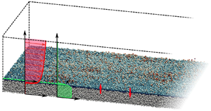
Figure 1. (a) Isometric view of a portion of the numerical domain. The uppermost layer of the particle bed is coloured by the particle's vertical location. Schematics of mean profiles of the streamwise component of the flow and volume fraction are shown in red and green, respectively. (b) The mean streamwise velocity profile as a function of  $z$ normalized by the boundary layer thickness $\delta$. Greyscale lines are from Voermans, Ghisalberti & Ivey (Reference Voermans, Ghisalberti and Ivey2017), with darker colours denoting less permeable granular beds. The blue line corresponds to case S0 (see table 1), which is the least permeable case considered. The simulation result is in reasonable agreement with the trend in the experiments.
The mean flow depth  $H_{f}^{\ast }$ and shear velocity $U_{\tau }^{\ast }$ are chosen as length and velocity scales, where $U_{\tau }^{\ast }$ is related to the mean streamwise pressure gradient as $U_{\tau }^{*2} = \nabla ^* P^* H_f^* /\rho _f^*$. The simulations consist of a particle bed composed of nearly 1.3 million particles of dimensionless diameter $d_p=d^{*}_p/H_{f}^{*} = 0.025$ below a unidirectional open-channel turbulent flow. The particle Stokes number may be defined from the particle terminal settling velocity $V_s^*$ (Kidanemariam & Uhlmann Reference Kidanemariam and Uhlmann2014) as $St=(\rho ^*_pV_s^*d_p^*)/(9\rho _f^*\nu ^*)$, where $V_s^*$ is given by the following implicit equation (Zgheib, Bonometti & Balachandar Reference Zgheib, Bonometti and Balachandar2015):
 \begin{equation} V_s^* = \frac{d_p^{*2}(\rho_p^*/\rho^*_f-1)g^*}{18\nu^*[1+0.15(V^*_sd^*_p/\nu^*)^{0.687}]}. \end{equation}
Five simulations are considered (see table 1). Here case S0 corresponds to the limiting case of immobile particles (i.e. small value of  $\varTheta /\theta _{cr}$). The submerged specific gravity of the sediment is chosen to be $R = \rho _p^*/\rho _f^* - 1 = 0.57$ to allow for comparison with the corresponding EE simulations of Zgheib et al. (Reference Zgheib, Fedele, Hoyal, Perillo and Balachandar2018a,Reference Zgheib, Fedele, Hoyal, Perillo and Balachandarb). The critical Shields number is computed as $\theta _{cr} = [0.22 Re^{-0.6}_p + 0.06 \exp (-17.77 Re^{-0.6}_p )]/2$ (Garcia Reference Garcia2008). The imposed flow is characterized by the Shields-like parameter $\varTheta = U^{*2}_{\tau }/(R \, g^{*} d^{*}_p)$. Since part of the applied pressure gradient will go to balance the form drag of the rough bed, $\varTheta$ will be larger than the mean streamwise shields stress $\langle \theta _x \rangle$ to be evaluated in the simulation, where in terms of the local streamwise shear stress $\theta _x=\tau ^*_x/[(\rho _p^*-\rho _f^*)\, g^{*} d^{*}_p]$. The bulk Reynolds number $Re_{bf}=U_{bf}^*H_f^*/\nu ^*$, where $U_{bf}^*=(1/H_f^*)\int _{H_b^*}^{H_b^*+H_f^*} \langle u^* \rangle \,\textrm {d}z^*$ is the mean fluid velocity above the bed–fluid interface. The values of $Re_{bf}$ and $St$ are given in table 1.
Table 1. Details of the numerical simulations. Here  $Re_p$ is the particle Reynolds number; $\theta _{cr}$ is the critical Shields number; $\varTheta$ is the Shields-like parameter of the imposed flow; $H_f^*$ is the mean flow depth and $H_b^*$ is the mean height of the bed above the bottom wall; $V_s^*$ is the particles’ terminal settling velocity (2.1); $St$ is the Stokes number; $Re_{bf}$ is the bulk Reynolds number. Dimensional parameters are denoted by an $(\cdot )^{*}$. Case S0 corresponds to immobile particles and therefore parameters associated with particle motion are irrelevant.

The permeability Reynolds number is defined as  $Re_k=\sqrt {K^*}U^*_{\tau }/\nu ^*$, where the permeability $K^*=(1-\phi )^3d_p^{*2}/(180\phi ^2)$ is estimated using the Carman–Kozeny model (Voermans et al. Reference Voermans, Ghisalberti and Ivey2017). In our simulations, the value of $\phi$ deep within the bed and away from the bed–fluid interface is around 0.62, which yields a low value of $Re_k = 0.13$. However, as will be discussed below, the KH vortices in the present simulations are observed only in selected regions of the bed where they penetrate to a depth of three particle diameters from the bed–fluid interface. Considering such a representative volume, we obtain a particle volume fraction of $\phi = 0.39$. Furthermore, the local shear stress in this high-speed region is 16 % higher than the global average. This yields $Re_k = 0.48$, which is still lower than the critical value for the observation of KH vortices in the recent experiments of Voermans et al. (Reference Voermans, Ghisalberti and Ivey2017). The difference could be perhaps due to the substantially smaller particles in the present simulations ( $d^{+}=3.74$) in comparison with the range used in the experiments ( $15\lessapprox d^{+}\lessapprox 250$). As can be seen from figure 1(b), the mean velocity profile qualitatively captures the trend observed in the experiments of Voermans et al. (Reference Voermans, Ghisalberti and Ivey2017) where the darker lines correspond to less permeable beds. The permeability of S0 is the lowest of all the cases in the frame. Quantitative differences are again perhaps due to the different particle sizes used in the simulations and the experiments.
Here and throughout the manuscript, the asterisk  $*$ denotes a dimensional quantity. The fluid phase mass and momentum conservation equations are
 \begin{equation} {\boldsymbol{\nabla}} \boldsymbol{\cdot} {\boldsymbol{u}} = -\frac{1}{\phi_f} \frac{\textrm{D} \phi_f}{\textrm{D} {t}}, \end{equation}
 \begin{equation}\frac{\textrm{D}{\boldsymbol{u}}}{\textrm{D}{t}} = \boldsymbol{G} -{\boldsymbol{\nabla}} {p} + \frac{1}{Re_{\tau}} {\nabla}^2 {\boldsymbol{u}} + \frac{{\boldsymbol{f}}_{pf}}{\phi_f}. \end{equation}
Here  $p$ is the dynamic pressure, $\phi _f= 1 - \phi$ and $\boldsymbol {u}$ are the volume fraction and velocity of the fluid phase, respectively. We impose a constant streamwise pressure gradient $\boldsymbol {G}=(1,0,0)$ and a shear Reynolds number $Re_{\tau } = U^{*}_{\tau } H^{*}_f / \nu ^* = 180$. Particle motion is computed by evaluating forces and torques and integrating the Newton–Euler equations. For details please refer to Finn, Li & Apte (Reference Finn, Li and Apte2016). Finally, $\boldsymbol {f}_{pf}$ represents the back-coupling force from the particles to the fluid.
The fluid and particle equations are solved using a highly scalable spectral element solver (Patera Reference Patera1984; Deville, Fischer & Mund Reference Deville, Fischer and Mund2002; Zwick & Balachandar Reference Zwick and Balachandar2020) in a domain of size  $L_x \times L_y \times L_z = 4{\rm \pi} \times 4{\rm \pi} /3 \times 1.31$ along the streamwise, spanwise and vertical directions. The domain is discretized using $30 \times 30 \times 13$ hexahedral elements with $11^3$ Gauss–Lobatto–Legendre (GLL) grid points within each element. The grid resolution varies with location and direction. In terms of $d_p$, the smallest (respectively, largest) grid spacing is in the vertical direction near the bed–fluid interface (respectively, along the flow direction) with a value of $0.0325d_p$ (respectively, $2.29d_p$). We also note that we do not apply any subgrid closure models. Data that is spatially averaged over the entire horizontal plane and over the interval $t=0.5$ to $t=2$ is denoted by $\langle \cdot \rangle$. We note that each simulation shown in table 1 corresponds to a unique set of physical parameters (Zgheib et al. Reference Zgheib, Fedele, Hoyal, Perillo and Balachandar2018a,Reference Zgheib, Fedele, Hoyal, Perillo and Balachandarb).
3. Results
3.1. Sediment flux
In figure 2(a), we show a scatter plot coloured by number density of  $q_{x}$ versus $( \theta _{x} -\theta _{cr})$ from S3, where $q_x$ is the streamwise component of local sediment flux. The data is plotted on a logarithmic scale along with WP correlation shown as the dashed line. The blue diamond symbol corresponds to $\langle q_{x}\rangle$ versus $(\langle \theta _{x} \rangle - \theta _{cr} )$. We observe a large scatter in the data spanning over several decades, yet we observe the mean value to match the WP model. In figure 2(b), we plot $\langle q_{x} \rangle$ versus $(\langle \theta _{x}\rangle -\theta _{cr})$. The open triangles correspond to MPM data corrected by Wong & Parker (Reference Wong and Parker2006) and therefore match with the dashed WP line. The + symbols correspond to MPM data, which along with the result of case S1 demonstrate that both MPM and WP correlations substantially underpredict the sediment flux when $\langle \theta _{x} \rangle$ is marginally in excess of $\theta _{cr}$.

Figure 2. (a) Scatter plot for  $q_x$ versus $(\theta _x-\theta _{cr})$ for S3 coloured by number density with a total number of bins of 62 500. The dashed green line corresponds to WP. The blue diamond symbol corresponds to $\langle q_x \rangle$ versus $(\langle \theta _x \rangle -\theta _{cr})$. Insets: probability distribution for $q_x$ and $(\theta _x-\theta _{cr})$, with blue (respectively, red) curve corresponding to the current EL (respectively, Zgheib et al. (Reference Zgheib, Fedele, Hoyal, Perillo and Balachandar2018a,Reference Zgheib, Fedele, Hoyal, Perillo and Balachandarb) EE) simulation; (b) $\langle q_x \rangle$ versus $(\langle \theta _x \rangle -\theta _{cr})$ for all simulations plotted against the WP (open triangles) and MPM original (+) data. The dashed and solid lines correspond to WP and MPM, respectively.
The scatter plots for all cases show qualitatively similar features: the largest  $q_x$ values are realized for a wide range of ( $\theta _{x}-\theta _{cr}$), and similarly a wide range of $q_x$ is realized close to the largest ( $\theta _{x}-\theta _{cr}$) values. The two most striking observations are: (i) small values of ( $\theta _{x} -\theta _{cr}$) are associated with the largest $q_x$, and (ii) small values of $q_{x}$ occur only during periods of intense turbulence marked by large values of ( $\theta _{x}-\theta _{cr}$). Both observations are counter intuitive at first glance. However, a closer look reveals that the larger particle flux is not always driven by large instantaneous excess Shields, but rather due to particles continuing their rapid downstream motion owing to their inertia, even after the turbulent structures that initiated their motion have departed. Only when this kinetic energy of particle motion is dissipated, the particle flux quickly decreases. On the other hand, upon the arrival of a leading intense vortical structure the shear stress quickly increases, but the particle flux may still remain small before its delayed response. It should be mentioned that there are few instances when local shear stress falls below the critical value (i.e. $\theta _{x}-\theta _{cr} < 0$) and similarly there are instances of negative $q_x$. These infrequent events are not captured in the log–log scatter plots.
We revisited the EE simulation results of Zgheib et al. (Reference Zgheib, Fedele, Hoyal, Perillo and Balachandar2018a,Reference Zgheib, Fedele, Hoyal, Perillo and Balachandarb) and evaluated the probability distribution function of  $\theta _x-\theta _{cr}$. The results shown in insets in panel (a) of figure 2 compare well with that of the corresponding Euler–Lagrange (EL) simulation S3. This clearly shows that the EE simulations, where the individual sediment grains are not distinguished as in the present EL simulations, are still able to reliably capture the turbulent shear stress variation. In comparison, substantial differences can be observed in the corresponding $q_x$ probability distribution function. The difference is in the inability of the EE approach to predict $q$ as a function of local $\theta$ using WP. The wider distribution of the present EL approach indicates that $q$ cannot be uniquely determined by the local and instantaneous Shields stress.
In figure 3, we show two subregions of the particle bed at  $t=0.9$ (the entire computational bed is later shown in figure 4). For both subregions five subpanels labelled (i)–(v) are shown. Figure 3(a i,b i) shows isocontours of volume fraction in the vertical plane bisecting the bed along with the bed-penetrating spanwise vortical structures observed therein. The white line marks the $\phi =0.1$ interface between the bed and the fluid. Figure 3(a ii,b ii) shows the vortical structures on the particle bed extracted with isosurfaces of swirling strength $\lambda _{ci}=20$ in the near-bed region. Figure 3(a iii,b iii) shows the regions where $q_x$ substantially deviates from what would be predicted by WP correlation using local excess Shields stress. The red (respectively, yellow) region corresponds to scatter plots where $q_x>q_{WP}+0.05$ (respectively, $q_x<q_{WP}-0.05$), with $q_{WP}$ being the prediction based on WP correlation using local $\theta _x - \theta _{cr}$. Figures 3(a iv,b iv) and 3(a v,b v) show isocontours of $q_x$ and $\theta _x-\theta _{cr}$, respectively.

Figure 3. Flow information at two subregions of the particle bed from S3 at  $t = 0.9$ displayed as five panels. (i) Isocontours of volume fraction in the vertical plane bisecting the bed in panel (ii) and penetrated by the same vortical structures observed therein. The white line marks the $\phi =0.1$ surface. (ii) View with particles coloured by $z$ location and overlain by KH rollers. (iii) Portions of the particle bed where $q_x$ is substantially larger (red), substantially smaller (yellow), or nearly equivalent (blue) to the corresponding WP value. (iv) Isocontours of $q_x$. (v) Isocontours of $\theta _x-\theta _{cr}$. The time history plot for $q_x$ and $\theta _x$ corresponds to point $C$ in panel (a ii).

Figure 4. Isometric view of the particle bed from S3 with three horizontal planes showing contours of streamwise velocity. The middle plane is located at the particle bed interface and denoted by  $\eta =z_{\phi =0.1}$. The other two planes are shifted by two particle diameters above and below the particle bed interface. Below the interface, only KH rollers are present, while above the interface, we only observe longitudinal streaks and do not detect the imprints of the KH rollers.
Starting with group A, we observe a region void of near-bed vortical structures at the downstream end of figure 3(a ii,b ii). This region is followed by a train of vortical structures. The yellow region in figure 3(a iii,b iii) is immediately below the leading vortical structure, while the red region is below the trailing part of the train of vortical structures. As the leading vortex sweeps over a region, it instantaneously increases the Shields stress as seen in figure 3(a v,b v). However,  $q_x$ does not immediately follow this increase in local Shields stress as seen in figure 3(a iv,b iv). Given enough time, and as the train of vortices sweeps over the same region and continues to do work on the particles, the yellow region in figure 3(a iii,b iii) turns red, i.e. particles that were already energized by the vortex structures that have moved downstream, continue to be accelerated by vortex structures that are currently overhead to yield a sediment flux much larger than what would be predicted by WP.
The temporal evolution of  $q_x$ (solid black line) and $\theta _x$ (red dashed line) at a point marked $C$ is shown in figure 3. The time lag between the two curves is clearly visible. The rise in the Shields number occurs as the first vortex sweeps over the point, however, particles do not immediately react, and we observe a delay in the rise of $q_x$. This time lag results in a large variation between the computed and the WP-predicted $q_x$. This temporal shift due to particle inertia is related to the spatial lag or saturation length between the location of change in shear stress to the point where a new equilibrium sediment flux is established (Charru Reference Charru2006; Parteli et al. Reference Parteli, Durán and Herrmann2007; Andreotti et al. Reference Andreotti, Claudin and Pouliquen2010). In point $C$ of figure 3, the temporal shift is approximately 0.047 non-dimensional units or $0.047U^*_{bf}/U^*_{\tau }=0.65$ bulk time units. The temporal shift not only depends on the particle size, but also on the past history of shear stress and work done on the particles. In general, the shift is pronounced only when the KH rollers are present.
On the other hand, we observe nearly the entire portion of the enlarged view B to be covered by vortical structures. Yet, the low sediment flux region, marked yellow in figure 3(a iii,b iii) does not appear at the same location over which the leading vortex acts, but farther upstream. This is in contrast to what was observed in figure 3(a iii) where the yellow region appears immediately below the leading vortex. Closer inspection of subpanel (i) reveals that the leading vortex in figure 3(b) does not penetrate into the particle bed (the green contour remains above the white line). This vertical separation between the leading vortex and the particle bed results in a relatively weaker influence on the latter. On the other hand, we observe the trailing vortices to dig well into the particle bed. In fact, it is at the location of the middle vortex that the yellow region emerges. Thus, the overall mechanism observed in figure 3(a) occurs in figure 3(b) as well. In figure 3, points where the relation between local  $q_x$ and excess Shields stress are in reasonable agreement with WP (i.e. $|q_x-q_{WP}|<0.05$) are marked blue in figure 3(a iii,b iii). Though there are turbulent vortical structures in these regions they do not represent coherent KH packets as observed in figure 3(a,b).
Coherent KH vortex structures that are substantially larger than individual pores or particles have been observed over permeable beds (e.g. Jimenez et al. Reference Jimenez, Uhlmann, Pinelli and Kawahara2001; Manes et al. Reference Manes, Poggi and Ridolfi2011; Suga, Mori & Kaneda Reference Suga, Mori and Kaneda2011; Kuwata & Suga Reference Kuwata and Suga2016, Reference Kuwata and Suga2017) and have been attributed to the presence of an inflection point in the mean streamwise velocity along the bed-normal direction (e.g. Jimenez et al. Reference Jimenez, Uhlmann, Pinelli and Kawahara2001; Breugem, Boersma & Uittenbogaard Reference Breugem, Boersma and Uittenbogaard2006). The porosity of the bed is necessary for these bed-penetrating coherent structures to form as they are not observed in wall-bounded flows over smooth or rough non-porous walls. Particle motion is also not important, since the KH vortices are observed even in case S0 of stationary particles. These KH vortices must be distinguished from the classical quasi-streamwise vortices and hairpin vortex packets that are observed to form and travel downstream in wall turbulence (e.g. Zhou et al. Reference Zhou, Adrian, Balachandar and Kendall1999; Cantero, Balachandar & Parker Reference Cantero, Balachandar and Parker2009). In fact, the inclined quasi-streamwise vortices and hairpin packets do not dig into the sediment bed.
Figure 4 shows the entire particle bed with individual grains coloured according to their elevation. To avoid obstructing the view of the bed, densely populated vortical structures, visualized as isosurfaces of  $\lambda _{ci}=20$ are only shown on one half of the bed. We plot contours of the fluid streamwise velocity $u$ at $z=\eta$, $\eta -2d_p$, and $\eta +2d_p$ (where $z=\eta$ is the bed interface identified as $\phi =0.1$). Well above the bed at $\eta +2d_p$, only classical high and low-speed streaks are seen (see the white contour lines projected on the panels below). Well inside the bed at $z=\eta -2d_p$ imprints of the KH rollers are seen as alternating red and blue stripes. Though the high and low-speed streaks are not visible in the colour contours at this elevation within the bed, the localization of the KH vortices at the highest shear regions of the high-speed streaks is clear. Both the streaks and the rollers are observed at $z=\eta$. At $z=\eta +2 d_p$, which is approximately eight wall units above the bed, just outside the viscous sublayer, the streamwise velocity contours are clearly indicative of the high- and low-speed streaks. The interpretation is that, in the present simulations, involving smaller sized particles, the KH vortices influence the high-speed streaks only within the viscous sublayer. The streamwise length of the streaks is observed to be approximately 887 wall units with a standard deviation of 175.7. The mean spacing between two adjacent high-speed streaks is approximately 103 wall units. These values are comparable to those observed in smooth and rough-wall turbulent channel flows (Jiménez & Moin Reference Jiménez and Moin1991; Jiménez & Pinelli Reference Jiménez and Pinelli1999; Bhaganagar, Kim & Coleman Reference Bhaganagar, Kim and Coleman2004).
The KH vortices are primarily located in the intense high-speed streaks due to the stronger shear-induced instability. The KH vortices are approximately four particle diameters in height, a dozen diameters in length and width. For the KH vortices to exist, bed porosity must allow the flow to penetrate in and out of the bed with streamwise passage in between. It must be emphasized that the clear signature of the KH vortices in figures 3 and 4 was possible only due to the coarse-graining of the flow implicit in the EL approach. In particle-resolved simulations (and in experiments), where this approximation is avoided, the KH vortices will be superposed with strong particle-scale perturbations and therefore will be harder to observe.
The high shear, combined with the porosity of the bed, is responsible for the KH vortices. Also, as described by the hairpin packet model of Zhou et al. (Reference Zhou, Adrian, Balachandar and Kendall1999), the streamwise propagation of the packet is the source of long high- and low-speed streaks (Adrian & Balachandar Reference Adrian and Balachandar2000), which are present even over a permeable bed. However, when the KH vortices coexist with the streaks, and with the disturbing influence of the individual particles, it may be that they cannot always be visualized in a straightforward way.
At any point on the bed, the arrival of bed-penetrating KH vortices swiftly increases the local Shields stress. However, because of particle inertia, sediment flux reacts only in a time-delayed fashion. A movie of the time evolution of figure 3(a iii,b iii) shows that the yellow and red regions of  $q_x$ remain coherent and advect with the flow. The local regions of above and below average $q_x$ change only as dictated by the advecting vortical structures. This suggests that the near-bed turbulent structures coupled with particle inertia are primarily responsible for the large scatter observed in figure 2. This also suggests that particle arrangement within the bed and pocket geometry play a lesser role.
3.2. Flow velocity at particle surface
An important consequence of KH vortices is that fluid and particle velocities at the bed–fluid interface evolve both temporally and spatially. We denote the streamwise and bed-normal components of fluid (respectively, particle) velocity at the bed surface as  $u_{bed}$ and $w_{bed}$ (respectively, $u_{p,bed}$ and $w_{p,bed}$). Figure 1 shows a schematic of $w_{bed}^+$ and ${w_{bed}^-}$. A non-zero fluid velocity at the bed surface has important implications on EE simulations, since most EE simulations use no-slip and no-penetration conditions (Janssen et al. Reference Janssen, Cardenas, Sawyer, Dammrich, Krietsch and De Beer2012; Broecker et al. Reference Broecker, Elsesser, Teuber, Özgen, Nützmann and Hinkelmann2018; Zgheib & Balachandar Reference Zgheib and Balachandar2019). We should note here that some EE simulations (Cheng, Hsu & Chauchat Reference Cheng, Hsu and Chauchat2018) consider the sediment–fluid interface to be the location where the sediment bed attains its maximum packing fraction. At that location, the fluid velocity amounts to only a small fraction of the bulk velocity. For such simulations, the use of a no-slip, no-penetration velocity boundary condition is likely be appropriate. Figure 5(a) shows $\langle u_{bed}\rangle$ and $\langle u_{p,bed}\rangle$ versus $\langle \theta _{x}\rangle -\theta _{cr}$. When $\langle \theta _{x} \rangle -\theta _{cr}\lessapprox 0.015$, $\langle u_{bed}\rangle$ attains a near-constant value and increases monotonically thereafter. The quadratic polynomial fit
 \begin{equation} \frac{\langle u_{bed}^* \rangle}{\sqrt{\langle \tau_x^* \rangle /\rho_f^*}} =150(\langle\theta_{x}\rangle-\theta_{cr})^2 - 0.62 (\langle\theta_{x}\rangle-\theta_{cr}) + 2.67 \end{equation}
adequately represents the trend. Even though the fit was derived for  $Re_{\tau }=180$, the results are likely to be valid for a wider range of $Re_{\tau }$ similar to the fact that the Wong & Parker (Reference Wong and Parker2006) relationship is also valid over a wide range of Reynolds number. Nevertheless, the applicability of the fit remains to be verified. In the inset of figure 5(a), we show the scatter plot coloured by number density for $u_{bed}$ versus $\theta _{x}-\theta _{cr}$ for case S3. The scatter shows that $u_{bed}$ spans a wide range from slightly negative values up to $75\,\%$ of the bulk velocity. The mean value of the scatter, shown by the blue diamond symbol, takes on a value of around 2.5, equivalent to nearly $16\,\%$ of the bulk velocity. It can be seen that the negative values of $\theta _{x}- \theta _{cr}$ predominantly correspond to positive $u_{bed}$ of substantial magnitude. Such data points suggest occasional significant value of $q_{x}$ even in regions of $\theta _{x} < \theta _{cr}$.

Figure 5. (a) Graph of  $\langle u_{bed} \rangle$ and $\langle u_{p,bed} \rangle$ versus $\langle \theta _x \rangle - \theta _{cr}$ using filled and open symbols, respectively. The line corresponds to the polynomial fit of $\langle u_{bed} \rangle$. Inset: scatter of $u_{bed}$ from S3 coloured by number density along with average value (cyan diamond). (b) Graph of $\langle w^+_{bed} \rangle / \langle u_{bed} \rangle$ and $\langle w^+_{p,bed} \rangle / \langle u_{p,bed} \rangle$ versus $\langle \theta _x \rangle - \theta _{cr}$ using filled and open symbols, respectively. Unlike panel (a) where spatial averaging is done for the entire horizontal plane, here spatial averaging is done exclusively over nodes with $w_{bed}>0$ and $w_{p,bed}>0$, respectively. Inset: scatter of $w_{bed}$ from S3 coloured by number density along with average value (cyan diamond). Total number of bins for each scatter plot is 62 500.
The variation of  $w_{bed}$ is also substantial when compared with the bulk streamwise flow (inset of figure 5b). The average of $w^+_{bed}$ over the respective area scaled by $\langle u_{bed} \rangle$ is plotted in figure 5(b). It is equivalent to the average over the negative component $w^-_{bed}$, and thus only the positive component is shown. In fact, it is observed that the positive and negative bed-normal velocities cover approximately 50 % of the bed each. This is to be expected since the total wall-normal velocity on any horizontal plane must be zero. We find the mean, positive and negative, bed-normal velocities to increase monotonically with excess Shields stress, but remain around $10\,\%$, compared with $u_{bed}$. The increase in $\langle u_{bed} \rangle$ and $\langle w^+_{bed} \rangle$ in figure 5 does not necessarily imply an increase in intensity and frequency of KH rollers but is likely a result of the elevated location $\eta$ for larger excess Shields stress values.
Particle streamwise and bed-normal velocities at the bed surface are also shown in figure 5 as open symbols. As expected, we observe the mean particle velocity to be smaller than the fluid velocity, since the latter drives the particle motion. The difference between the two indicates the slip velocity between the particle and the fluid near the bed surface. We should note that the randomly distributed KH vortex packets are present in all cases considered, and they appear to be of comparable strength. Even under intense bedload transport, we observe the fluid velocity to be locally larger than the sediment velocity. Furthermore, the two main ingredients needed for KH vortices, namely bed porosity and mean shear in the fluid velocity profile, are present even under strong bedload transport. However, it is not clear if the intensity of the KH vortices will increase or decrease with further increase in excess Shields stress.
4. Conclusions
We presented results from EL simulations of turbulent flow over a mobile particle bed. From a global perspective, our simulations correctly reproduce the WP relation of bedload transport. However, large variations, up to a few orders of magnitude, between the computed and WP-estimated sediment flux ( $q_x$) are observed at the instantaneous and local level. These large variations are attributed primarily to the combined effects of particle inertia and bed-penetrating KH vortices. The influence of particle bed arrangement or pocket geometry was observed to play a lesser role. The EE simulations (Zgheib et al. Reference Zgheib, Fedele, Hoyal, Perillo and Balachandar2018a,Reference Zgheib, Fedele, Hoyal, Perillo and Balachandarb) can reliably reproduce turbulent shear stress variations observed in the present EL simulations, provided the particle diameter is sufficiently small. However, $q_x$ predicted based on WP correlation will exhibit far lower variation than the EL counterpart. Models that account for the past history of the Shields stress $\theta$ and the inertial behaviour of particles must be developed for improved prediction. Additionally, an important consequence of KH vortices is that fluid and particle velocities at the bed surface are non-zero but are temporally and spatially evolving quantities. A simple quadratic correlation is presented for the mean streamwise fluid velocity applicable at the bed–fluid interface. Finally, we note that the results related to the KH instability require experimental validation.
Supplementary movie
Supplementary movie is available at https://doi.org/10.1017/jfm.2020.1060.
Acknowledgements
The authors gratefully acknowledge support from ExxonMobil Upstream Research Company through grant number EM09296. The simulations were performed with the help of the High Performance Computing Center at the University of Florida. The authors are also grateful to the three anonymous reviewers for improving the quality of the manuscript, and to M. Uhlmann, C. Manes and M. Mazzuoli for fruitful discussions.
Declaration of interests
The authors report no conflict of interest.


 Open access