


1. Introduction
Turbulent buoyant jets and plumes are found in a wide range of natural and engineering problems, including deep-sea hydrothermal vents, volcanic eruptions, fire plumes, condenser cooling water and products of combustion processes in wildfires and industrial burners (Lee & Chu Reference Lee and Chu2012; Heskestad Reference Heskestad2016). In many of these problems, it would be prohibitively expensive to numerically model all relevant scales of motion by directly and exactly solving the Navier–Stokes equations. Consequently, a primary objective of research on these flows has been to accurately model flow properties using simpler equation sets, either by reducing the full set of partial differential equations into a set of ordinary differential equations, or by modelling unclosed terms in Reynolds-averaged Navier–Stokes simulations or large-eddy simulations. However, there are currently no reduced models that are universally accurate over the wide range of conditions observed in real-world applications.
To date, most studies of buoyant jets and plumes have focused primarily on far-field properties. Considering, for example, axisymmetric buoyant jets and plumes flowing primarily in the vertical direction against gravity, the seminal study by Morton, Taylor & Turner (Reference Morton, Taylor and Turner1956) (denoted MTT henceforth) provided far-field predictions based on the following assumptions: (i) the time-averaged vertical velocity and buoyancy profiles are self-similar (e.g. Gaussian) at all vertical locations; (ii) the rate of entrainment at the edge of the flow is proportional to a characteristic velocity; (iii) the flow is statistically steady; (iv) average pressure gradients in the vertical direction are much greater than in the transverse direction; (v) the Reynolds number is high, placing the flow in the fully turbulent regime; (vi) there is negligible mass and thermal diffusion; and (vii) the largest local density variations are small compared with the ambient density (Hunt & van den Bremer Reference Hunt and van den Bremer2011). Using these assumptions, the continuity and Navier–Stokes equations can be reduced to a set of ordinary differential equations that describe the time-averaged fluxes of volume, momentum and buoyancy through transverse planes (Hunt & Kaye Reference Hunt and Kaye2005). These ordinary differential equations are
 \begin{equation} \frac{\mathrm{d} {\mathcal{Q}}}{\mathrm{d} z} = 2 \alpha {\mathcal{J}}^{1/2}, \quad \frac{\mathrm{d} {\mathcal{J}}}{\mathrm{d} z} = 2 \frac{{\mathcal{Q}}\,{{\mathcal{B}}}}{{\mathcal{J}}}, \quad \frac{\mathrm{d} {\mathcal{B}}}{\mathrm{d} z} = 0, \end{equation}
where  $z$ is the vertical location, $\alpha$ is an entrainment coefficient that is generally assumed to be constant (Hunt & Kaye Reference Hunt and Kaye2005; van Reeuwijk & Craske Reference van Reeuwijk and Craske2015; Ciriello & Hunt Reference Ciriello and Hunt2020) and ${\mathcal {Q}}$, ${\mathcal {J}}$ and ${\mathcal {B}}$ are the time-averaged volume, momentum and buoyancy fluxes, respectively.
These equations, which are derived in detail by Hunt & van den Bremer (Reference Hunt and van den Bremer2011), have proven useful for describing the far-field characteristics of jets, plumes and forced plumes (also known as buoyant jets), as shown by Papanicolaou & List (Reference Papanicolaou and List1988) and Shabbir & George (Reference Shabbir and George1994). Using dimensional analysis, these equations can be used to determine the scaling relationships of the fluxes or flow variables for three-dimensional jets and plumes as
 \begin{gather} \text{pure jets:} \quad {\mathcal{Q}} \sim z, \quad {\mathcal{J}} \sim \text{const.},\quad {\mathcal{B}}=0, \quad \delta \sim z, \quad u_{c} \sim z^{{-}1}, \end{gather}
 \begin{gather}\text{pure plumes:} \quad {\mathcal{Q}} \sim z^{5/3}, \quad {\mathcal{J}} \sim z^{4/3},\quad {\mathcal{B}}\sim\text{const.}, \quad \delta \sim z, \quad u_{c} \sim z^{{-}1/3}, \end{gather}
where  $\delta$ is a characteristic time-averaged flow width and $u_{c}$ is the time-averaged centreline vertical velocity (List Reference List1982; Lee & Chu Reference Lee and Chu2012). Similar scaling relationships can also be found for non-Boussinesq plumes with an additional density ratio variable (Rooney & Linden Reference Rooney and Linden1996).
In forced plumes, where the momentum flux is larger than the buoyant flux at the inlet, Papanicolaou & List (Reference Papanicolaou and List1988) showed that there is a transition from jet-like scaling to plume-like scaling; this transition was subsequently derived analytically by Diez & Dahm (Reference Diez and Dahm2007). From these results, it is possible to deduce a ‘virtual origin’, or an ideal point source of momentum and/or buoyancy flux with initially no mass flux, that entrains fluid such that upon reaching the  $z$ location of the finite-area source, the flow emanating from the virtual origin has the same fluxes as the finite-area source. This can then be used to predict flow properties in the far field.
Although MTT theory has been successfully applied to jets, plumes and forced plumes, it is not immediately applicable to ‘lazy’ plumes where the buoyancy flux is greater than the momentum flux at the inlet and the assumptions underlying MTT theory become invalid, particularly in the near field (Turner Reference Turner1986). Caulfield (Reference Caulfield1991) showed that, by rewriting the governing equations in terms of a flux-based Richardson number and numerically solving the resulting single equation, it is possible to capture certain essential features of the near-field plume, including ‘necking’ of the flow immediately above the inlet. The necking phenomenon only occurs in lazy plumes and the location where it occurs has been predicted analytically by Hunt & Kaye (Reference Hunt and Kaye2005) using the procedure they proposed in an earlier study (Hunt & Kaye Reference Hunt and Kaye2001). However, Kaye & Hunt (Reference Kaye and Hunt2009) later showed experimentally that entrainment can be described by a linear scaling of volume flux with respect to the downstream distance, contradicting previous theoretical work. This scaling was further supported by the two-dimensional numerical simulations of Jiang & Luo (Reference Jiang and Luo2000b). Thus, while necking can be predicted by the MTT theory, the theory itself is not generally applicable to lazy plumes without additional modifications to account for near-field flow features, such as the puffing instability; further generalizations of MTT have been proposed to account for variable entrainment and unsteadiness in lazy plumes (Kaminski, Tait & Carazzo Reference Kaminski, Tait and Carazzo2005; van Reeuwijk & Craske Reference van Reeuwijk and Craske2015; Carlotti & Hunt Reference Carlotti and Hunt2017; Ciriello & Hunt Reference Ciriello and Hunt2020).
To develop more accurate models and theories for the near-field dynamics of lazy plumes, similar to those provided by the MTT theory for the far-field dynamics, we require a more detailed understanding of near-field volume, momentum and buoyancy fluxes across a range of conditions. Experimentally, there have been many studies of the near field of buoyant plumes (Hamins, Yang & Kashiwagi Reference Hamins, Yang and Kashiwagi1992; Cetegen & Kasper Reference Cetegen and Kasper1996; Cetegen Reference Cetegen1997; Colomer, Boubnov & Fernando Reference Colomer, Boubnov and Fernando1999; Friedl, Härtel & Fannelop Reference Friedl, Härtel and Fannelop1999; Epstein & Burelbach Reference Epstein and Burelbach2001; O'hern et al. Reference O'hern, Weckman, Gerhart, Tieszen and Schefer2005; Bharadwaj & Das Reference Bharadwaj and Das2017). However, these studies have focused primarily on flow statistics and the characteristic oscillatory motion by which coherent vortical structures are periodically shed, often referred to as ‘puffing’. The only experimental study that quantifies fluxes in buoyant plumes is that of Kaye & Hunt (Reference Kaye and Hunt2009), who found a linear correlation of volume flux with downstream distance (although the experimental configuration only supported small density fluctuations).
With recent advances in computational power and techniques, highly resolved three-dimensional numerical simulations have been performed for buoyant jets and plumes without the use of a subgrid-scale model, which we term direct numerical simulations (DNS). Taub et al. (Reference Taub, Lee, Balachandar and Sherif2015) and Marjanovic, Taub & Balachandar (Reference Marjanovic, Taub and Balachandar2017, Reference Marjanovic, Taub and Balachandar2019) provide detailed statistical information from DNS, with a particular emphasis on quantifying higher-order statistics and comparing their data with existing theoretical predictions under the Boussinesq approximation. Some DNS are available using a low-Mach approximation (Jiang & Luo Reference Jiang and Luo2000a,Reference Jiang and Luob; Nichols, Schmid & Riley Reference Nichols, Schmid and Riley2007; Wimer et al. Reference Wimer, Day, Lapointe, Meehan, Makowiecki, Glusman, Daily, Rieker and Hamlington2021), but most of these studies focus primarily on temporal characteristics and puffing. Of these, the only DNS study to comment on fluxes is that of Jiang & Luo (Reference Jiang and Luo2000b), who found that the mass flux in both axisymmetric and planar two-dimensional buoyant plumes varies approximately linearly with vertical location.
In the present study, we use three-dimensional DNS to examine flow statistics and fluxes in the near field of lazy plumes with large density differences. We focus on the dependence of the average flow structure (quantified using first- and second-order moments) and average fluxes on the inlet Richardson and Reynolds numbers. Previous studies have shown that the Richardson number has a leading-order effect on the temporal dynamics of the flow (Cetegen & Kasper Reference Cetegen and Kasper1996; Wimer et al. Reference Wimer, Lapointe, Christopher, Nigam, Hayden, Upadhye, Strobel, Rieker and Hamlington2020), but less is known about the dependence of fluxes on this non-dimensional parameter. The Reynolds number does not appear in any of the theoretical predictions of flux behaviour or in prior empirical relationships for the puffing frequency, primarily because theoretical developments assume a high-Reynolds-number flow. However, many buoyant plumes are not necessarily of high Reynolds number (Hunt & Kaye Reference Hunt and Kaye2001), and it is important to understand the conditions for which the flow transitions to turbulence. Additionally, the Reynolds number controls small-scale structure for many fluid instabilities, including the Rayleigh–Taylor (RT) instability (Wei & Livescu Reference Wei and Livescu2012), which is likely the most relevant fluid instability in the near field of lazy plumes (O'hern et al. Reference O'hern, Weckman, Gerhart, Tieszen and Schefer2005).
Although our focus here is only on Richardson and Reynolds number effects, it is likely that the present results also depend on other non-dimensional numbers. Of these, the Atwood number (or some other equivalent density-based non-dimensional number) is likely to be an important parameter in dictating the average plume structure. This can be anticipated from studies of non-Boussinesq plumes (Ricou & Spalding Reference Ricou and Spalding1961; Rooney & Linden Reference Rooney and Linden1996), as well as from studies of asymmetric mixing in RT instabilities (Livescu et al. Reference Livescu, Ristorcelli, Petersen and Gore2010). However, here we perform all simulations with helium and air, resulting in a large Atwood number relevant to reacting plumes, where the formation of hot combustion products results in a density ratio roughly equivalent to that of helium and air (Cetegen & Ahmed Reference Cetegen and Ahmed1993). Exploration of different Atwood numbers, including very small values where Boussinesq plume theory would be more applicable, is an important direction for future work, but we do not pursue this here.
In the next section, we provide a brief discussion of the numerical simulations, which are performed using adaptive mesh refinement (AMR) in the low-Mach code PeleLM (Day & Bell Reference Day and Bell2000; Nonaka, Day & Bell Reference Nonaka, Day and Bell2018). In § 3, we present statistics computed from the simulations. We discuss the results in § 4, with a particular emphasis on providing theoretical support for the results in § 3. We then conclude in § 5.
2. Numerical simulations
We perform numerical simulations of three-dimensional helium buoyant plumes using the low-Mach governing equations as described by Rehm & Baum (Reference Rehm and Baum1978) and Majda & Sethian (Reference Majda and Sethian1985). These equations allow for density variations due to molecular mixing but not from pressure variations. We solve the governing equations using PeleLM (Nonaka et al. Reference Nonaka, Day and Bell2018), a scalable hydrodynamics code that uses AMReX, a software framework for block-structured AMR (Zhang et al. Reference Zhang2019). The simulations analysed here are the same as those described in Meehan, Wimer & Hamlington (Reference Meehan, Wimer and Hamlington2022), where we also provide a more extensive description of the numerical implementation.
To model the plumes, we use a Dirichlet boundary condition at  $z=0$ m (i.e. the bottom of the domain) that represents a circular region of radius $R_0=0.125$ m where pure helium is injected into the domain at a prescribed inflow velocity, $U_0$. There is no co-flow and the rest of the bottom boundary is modelled as a no-slip wall. At the helium–air interface on the bottom boundary, we use a hyperbolic tangent profile with smoothing factor $\phi = 2.5\times 10^{-3}$ m to smoothly transition the inflow velocity and properties into the quiescent air (Michalke Reference Michalke1984; Meehan et al. Reference Meehan, Wimer and Hamlington2022). The fluids are fixed at a temperature of $T=300$ K. The remaining five computational boundaries are modelled as Neumann boundary conditions to allow air to be entrained through the side boundaries and the helium–air mixture to convect out of the top boundary.
To examine effects due to varying inlet Richardson,  ${Ri}_0=(1-\rho _0/\rho _\infty )g R_0/U_0^2$, and Reynolds, ${Re}_0=\rho _0 U_0 R_0/\mu _0$, numbers, the gravitational acceleration, $g$, and $U_0$ were varied while fixing the remaining parameters. In total, 18 different simulations were performed, spanning ${Ri}_0$ between 2 and 63, and ${Re}_0$ between 100 and 1000. We vary $U_0$ and $g$ in the simulations to independently vary ${Ri}_0$ and ${Re}_0$ while maintaining $R_0$ constant. The computational domain is large enough (either 1.5 or 2.0 m to a side, with a height equal to the side length) to ensure that flow features of interest are far from the outer computational boundaries and AMR is used to add grid resolution where required.
All statistics are computed using approximately 100 turnover times based on the period of the puffing oscillations in each simulation,  $\tau ^*=1/f^*$, where $f^*$ is the expected puffing frequency from the relation $f^* R_0/U_0=2e^{-1} ({Ri}_0/2)^{2/5}$ (Wimer et al. Reference Wimer, Lapointe, Christopher, Nigam, Hayden, Upadhye, Strobel, Rieker and Hamlington2020). Statistics were collected only after letting the flow develop for approximately $20\tau ^*$, which is when the flow was found to have achieved a statistically stationary state. Table 1 provides a summary of the parameters and conditions for the simulations examined in this study.
Table 1. List of dynamically relevant parameters used to determine the inlet Richardson,  ${Ri}_0= (1-\rho _0/\rho _\infty ){gR_0}/{U_0^2}$, and Reynolds, ${Re}_0 = {\rho _0 U_0 R_0}/{\mu _0}$, numbers in the buoyant plume simulations. Values in the third column prefaced with $\approx$ are only approximate. The complete set of parameters for all simulations is provided in Meehan et al. (Reference Meehan, Wimer and Hamlington2022).

Additional details of the AMR strategy used in the simulations, including detailed convergence tests, are provided in Meehan et al. (Reference Meehan, Wimer and Hamlington2022). Briefly, vorticity and cell-to-cell density differences were used to determine where grid refinement should occur, and three levels of refinement were used to resolve the flow to a finest resolution of just under 2 mm. This resolution was also shown in Wimer et al. (Reference Wimer, Lapointe, Christopher, Nigam, Hayden, Upadhye, Strobel, Rieker and Hamlington2020, Reference Wimer, Day, Lapointe, Meehan, Makowiecki, Glusman, Daily, Rieker and Hamlington2021) to be sufficient for capturing the mean flow structure and dynamics in buoyant plumes similar to those examined here.
It should be noted that the numerical simulations were performed in a Cartesian coordinate system; however, the spatial statistical symmetry of the flow is in the azimuthal direction for a cylindrical coordinate system with origin at the centre of the inlet (i.e. the flow is statistically axisymmetric). To maximize the statistical convergence of the moments and fluxes computed here, we use both temporal and azimuthal averages, requiring appropriate transformations from Cartesian to cylindrical coordinates for non-scalar quantities (e.g. velocity components). The interchanging of coordinate systems and the presence of varying grid resolution due to the AMR also require a series of interpolation steps to compute averages and fluctuations. This can result in large errors if appropriate measures are not taken in the interpolation method. In Appendix A, we outline a space-filling nearest-neighbour interpolation strategy for azimuthal averages and use an Akima spline strategy (De Boor Reference De Boor1978) for the averaged fields needed to compute fluctuating variables.
3. Results
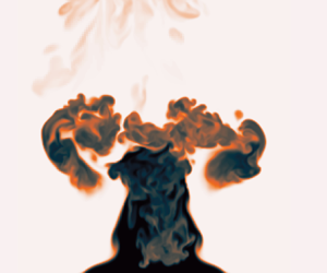
Qualitative characteristics of the simulated plumes are indicated in figure 1, which shows time series of the density field over a time span of  $\tau ^*$ for ${Re}_0=100$, $316$ and $1000$, all at ${Ri}_0=6.3$. For each ${Re}_0$, there is a buoyancy-driven acceleration of the helium at the base of the plume, leading to a contraction of the flow and the formation of vortical structures. This process repeats in a periodic manner, leading to the characteristic puffing behaviour widely observed in buoyant plumes; the temporal characteristics of these plumes are the primary focus of Meehan et al. (Reference Meehan, Wimer and Hamlington2022).

Figure 1. Time series of the density field over  $\Delta t \approx \tau ^*$ at ${Ri}_0=6.3$ for ${Re}_0=100$ (a–e), ${Re}_0=316$ (f–j) and ${Re}_0=1000$ (k–o). Panels (a,f,k) show where the grid is refined, with grey indicating two levels of refinement and black indicating three levels of refinement. Panels (e,j,o) include the in-plane direction of the velocity vector (not scaled with velocity magnitude).
Figure 1 also shows the transition from laminar to turbulent flow. As  ${Re}_0$ increases, increasingly fine vortices are formed and there is penetration of air into the core of the plume, increasing the density along the centreline. This is clearest in figure 1(k), where the density is higher due to mixing with ambient air along the centreline near the inlet. This penetration of high-density ambient fluid is similar to the formation of downward-propagating high-density ‘spikes’ observed in classical RT instabilities.
In the following, we examine the dependence of the plumes on  ${Ri}_0$ and ${Re}_0$ by considering statistics of the vertical velocity and density, as well as average fluxes. The averaging and interpolation procedure outlined in Appendix A is used to calculate all statistics and fluxes.
3.1. First-order velocity and density statistics
Figure 2 shows  $r$–
$r$– $z$ fields of average vertical velocity, $\bar {u}_z/U_0$, and density, $\bar {\rho }/\rho _0$, for ${Ri}_0=6.3$ and all ${Re}_0$, where the overline indicates an azimuthal and temporal average. Immediately above the inlet, the flow narrows and accelerates vertically, as is also indicated by the profiles of centreline vertical velocity $u_{c}(z)\equiv \bar {u}_z(r=0,z)$ in figure 3. This figure shows that, as ${Ri}_0$ increases, the location of peak $u_{c}$ generally decreases for all ${Re}_0$, while the smallest value of ${Ri}_0$ in figure 3(a) shows that the lowest values of ${Re}_0$ have increasing $u_{c}$, even at $z/R_0=5$.

Figure 2. Time and azimuthal averages of vertical velocity  $\bar {u}_z/U_0$ (a–e) and density $\bar {\rho }/\rho _0$ (f–j) for ${Ri}_0=6.3$ and (a,f) ${Re}_0=100$, (b,g) ${Re}_0=178$, (c,h) ${Re}_0=316$, (d,i) ${Re}_0=562$ and (e,j) ${Re}_0=1000$. Dashed lines are contours of velocity- and density-based flow widths, $\delta _u/2R_0$ (a–e) and $\delta _\rho /2R_0$ (f–j), respectively.

Figure 3. Centreline average vertical velocity  $u_{c}/U_0$ (a–d) and centreline average density $\rho _{c}/\rho _0$ (e–h) for (a,e) ${Ri}_0=2$, (b,f) ${Ri}_0=6.3$, (c,g) ${Ri}_0=20$ and (d,h) ${Ri}_0=63$. Line colours correspond to different Reynolds numbers, ${Re}_0$.
Both figures 2 and 3 show that, for  ${Ri}_0=6.3$, the ${Re}_0=178$ plume accelerates up to at least $z/R_0=5$, with the ${Re}_0=100$ case having a maximum $u_{c}$ at $z/R_0\approx 3\unicode{x2013}4$ and the three highest values of ${Re}_0$ having peak velocities at $z/R_0\approx 2\unicode{x2013}3$. This non-monotonicity in $u_{c}$ with increasing ${Re}_0$ is a result of the complex vortex dynamics that arises in the puffing instability as the flow transitions from laminar to turbulent; this transition is discussed in more detail in Meehan et al. (Reference Meehan, Wimer and Hamlington2022). As ${Ri}_0$ increases, figure 3 shows that changes in $u_{c}$ become monotonic with increasing ${Re}_0$ (e.g. in the ${Ri}_0=20$ and 63 cases).
Corresponding trends are observed for  $\bar {\rho }$ in the bottom rows of figures 2 and 3, where the increase in $\bar {\rho }$ becomes more rapid along the centreline as both ${Ri}_0$ and ${Re}_0$ increase. Once again, for the two lowest values of ${Ri}_0$, the centreline profile $\rho _{c}(z)\equiv \bar {\rho }(r=0,z)$ is smallest for ${Re}_0=178$, reflecting the non-monotonicity in the trends of $u_{c}$ with increasing ${Re}_0$ at low ${Ri}_0$. For the two largest values of ${Ri}_0$ in figure 3, the trends in $\rho _{c}$ are monotonic with increasing ${Re}_0$.
Figure 3 shows that there is an additional flow transition as the core of the plume is penetrated by heavier ambient fluid for  ${Ri}_0=20$ with ${Re}_0>100$, and ${Ri}_0=63$ for all ${Re}_0$. This phenomenon is distinguished by the abrupt change in $\rho _{c}$ near $z=0$ (e.g. in figure 3h) and by negative values of $u_{c}$ in the very near field. That is, the penetration of heavier fluid becomes so strong that, on average, there is a recirculation zone along the centre of the plume, marked by $u_{c}<0$. This penetration is reminiscent of that found in RT instabilities and, henceforth, we refer to this phenomenon as a RT ‘spike’. This penetration is particularly remarkable because, despite the plume having a non-zero upward injection of helium, the spikes are strong enough to create recirculation.
Flow widths can also be computed from the average vertical velocity and density fields. The contours  $\delta _u/2R_0$ and $\delta _\rho /2R_0$ are shown in figure 2, where $\delta _\varphi$ is the flow width corresponding to the radial location at which the average variable of interest, $\overline {\varphi }$, has decreased (increased) by 50 % from its centreline value for vertical velocity (density). This definition is used so that each flow width is roughly equivalent to the nominal diameter at the inlet; i.e. $\delta _\rho (z=0) \approx \delta _u(z=0) = 2R_0$.
The contours in figure 2 indicate how the flow necks, corresponding to a contraction and expansion of the flow as a function of vertical location. Quantitatively, the neck is defined as the minimum flow width and the vertical profiles of  $\delta _u$ and $\delta _\rho$ in figure 4 reveal that the neck is typically in the range $z/R_0 \approx 1\unicode{x2013}2$. Below the neck, the flow rapidly contracts, shrinking the width and increasing the centreline velocity. Above the neck, turbulent mixing increases and both the vertical velocity and density discrepancy (i.e. $\rho _{c}-\rho _0$) along the centreline diminish. Generally, the peak in $u_{c}$ occurs at the neck location.

Figure 4. Flow widths based on the average vertical velocity  $\delta _u$ (a–d) and average density $\delta _\rho$ (e–h) for (a,e) ${Ri}_0=2$, (b,f) ${Ri}_0=6.3$, (c,g) ${Ri}_0=20$ and (d,h) ${Ri}_0=63$. Marker shapes and colours correspond to different Reynolds numbers, ${Re}_0$.
Figure 4 allows us to directly compare  $\delta _u$ and $\delta _\rho$ for different ${Re}_0$ for each ${Ri}_0$, where all figure panels also have the same axes to facilitate additional comparisons between different ${{Ri}_0}$ and flow width definitions. Very close to the inlet for $z/R_0\lesssim 0.5$, $\delta _u$ and $\delta _\rho$ are very similar for different ${Re}_0$. Farther downstream, the flow widths increase after the neck is reached, where larger ${Re}_0$ generally results in larger flow widths. Sufficiently far downstream in the more turbulent cases, $\delta _u$ and $\delta _\rho$ generally become similar for different ${Re}_0$. This is most apparent for ${Ri}_0 = 20\unicode{x2013}63$ at $z/R_0 \approx 4\unicode{x2013}5$. Near the inlet at locations below $z\approx R_0$, there is good agreement between $\delta _u$ and $\delta _\rho$ for different ${Re}_0$, with better agreement for low ${Re}_0$ when the flow is laminar. However, the flow widths diverge for higher ${Re}_0$, which is likely associated with the breakdown of the shear layer and vortex roll-up via Kelvin–Helmholtz instability. The neck locations computed from the minima of $\delta _u$ and $\delta _\rho$ converge to $z\approx R_0$ as ${Ri}_0$ and ${Re}_0$ increase, consistent with the experiments of Epstein & Burelbach (Reference Epstein and Burelbach2001). This consistency between different flow widths has been observed previously in the far field of pure plumes (Craske, Salizzoni & van Reeuwijk Reference Craske, Salizzoni and van Reeuwijk2017), but this is the first time that it has been shown in the near field of lazy plumes with large density differences.
The dependence of the average radial plume structure on  ${Ri}_0$ and ${Re}_0$ is indicated in figures 5 and 6. Note that the profiles in figure 5 are normalized by the local centreline velocity, $u_c$, and the local flow width, $\delta _u$, while in figure 6 the profiles are normalized by fixed inlet values. In figure 5, we show the radial profiles of $\bar {u}_z$ for different vertical locations, and we include the top-hat profile used for the inlet and a Gaussian profile using the plume width. From these profiles, it can be seen that there is a transition from a smoothed top-hat profile at the inlet to a far-field Gaussian profile with increasing vertical distance. The Gaussian profile is associated with far-field plume scaling, and all cases in figure 5 approximately attain far-field behaviour by $z/R_0=5$.

Figure 5. Radial profiles of  $\bar {u}_z$ normalized by $u_{c}$ for (a,e,i) ${Ri}_0=2$, (b,f,j) ${Ri}_0=6.3$, (c,g,k) ${Ri}_0=20$ and (d,h,l) ${Ri}_0=63$ at vertical locations $z/R_0=0.5$ (a–d), $z/R_0=2$ (e–h) and $z/R_0=5$ (i–l). Line colours correspond to different ${Re}_0$. Dashed lines are the smoothed top-hat velocity profile prescribed at the inlet and dash-dotted lines are Gaussian profiles expected in the far field.

Figure 6. Radial profiles of  $\bar {\rho }$ normalized by $\rho _0$ for (a,e,i) ${Ri}_0=2$, (b,f,j) ${Ri}_0=6.3$, (c,g,k) ${Ri}_0=20$ and (d,h,l) ${Ri}_0=63$ at vertical locations $z/R_0=0.5$ (a–d), $z/R_0=2$ (e–h) and $z/R_0=5$ (i–l). Line colours correspond to different ${Re}_0$.
This transition, however, is complicated by the presence of coherent structures associated with the puffing instability. This can be seen most clearly in figure 6 where we show radial profiles of  $\bar {\rho }$ at the same vertical locations as in figure 5. At $z=R_0/2$, there is a small plateau in the density profile along the shear layer as a result of the puffing instability. Additionally, the low- ${Re}_0$ profiles show that there is no mixing near the centreline while the higher- ${Re}_0$, more turbulent, cases do mix, consistent with the observation that RT spikes penetrate into the core of the plume and increase helium–air mixing. Higher above the inlet, helium continues to mix with air, with generally greater mixing as ${Ri}_0$ and ${Re}_0$ increase (although some non-monotonicity is present, consistent with results from figures 3 and 4). Lastly, plumes with RT spikes have greater mixing rates; this can be seen most clearly for the ${Ri}_0=20$ case where there are no RT spikes for ${Re}_0=100$ and as the flow propagates downstream, the mixing is slower than larger ${Re}_0$ with RT spikes.
Figure 5 shows that there is a distinctive peak in  $\bar {u}_z$ away from the centreline near the inlet (i.e. at $z/R_0=0.5$) for all ${Ri}_0$ and sufficiently high ${Re}_0$. This off-centre peak is the result of the rapid acceleration that occurs along the shear layer where the two fluids interact, as well as the formation of downward-propagating high-density ambient fluid into the core of the plume associated with RT spikes.
We further examine these off-centre peaks in figure 7, which shows the radial location of maximum  $\bar {u}_z$ at each vertical location, coloured by the relative magnitude of the maximum velocity in the radial direction at each $z$ (i.e. $\max _r(\bar {u}_z)/u_{c}$). For each ${Ri}_0$, the locations of maximum velocity are in good agreement for all ${Re}_0$. However, with increasing ${Re}_0$, the ratio $\max _r(\bar {u}_z)/u_{c}$ increases substantially and, as ${Ri}_0$ increases, the ratio increases more quickly. This highlights the important role of ${Re}_0$ in determining the average structure of lazy plumes, even for highly turbulent conditions.

Figure 7. Radial locations of maximum  $\bar {u}_z$ at each vertical location $z$ for (a) ${Ri}_0=2$, (b) ${Ri}_0=6.3$, (c) ${{Ri}_0=20}$ and (d) ${Ri}_0=63$. Colour indicates the value of $\max _r[\bar {u}_z(r,z)]/u_{c}(z)$ at each $z$. Shapes correspond to different ${Re}_0$ according to the legend in (a).
3.2. Second-order velocity and density statistics
Second-order fluctuating statistics of velocity and density appear in higher-order models of plume dynamics that account for deviations from MTT theory, such as in van Reeuwijk & Craske (Reference van Reeuwijk and Craske2015), and can also be used to characterize the intensity of turbulent fluctuations in the flow. In the following, we use the buoyancy-based velocity scale  $(gR_0)^{1/2}$ to normalize $u_i$ because of the important role played by gravity in destabilizing the flow and causing variability. We found that this scale provided a better collapse of the data between different ${Ri}_0$ than $U_0$. Density is normalized in all cases by $\rho _\infty$.
Figure 8 shows radial profiles of all non-zero second-order moments formed from the fluctuating density  $\rho '$ and the fluctuating velocities $u'_r$, $u'_\theta$ and $u'_z$ at $z=R_0/2$. This vertical location is within the region of the flow dominated by the puffing and each of the fluctuating variables is calculated with respect to azimuthal and temporal averages as $\varphi '=\varphi -\overline {\varphi }$.

Figure 8. Second-order statistics at  $z=R_0/2$ of (a–d) $\overline {\rho '\rho '}/\rho _\infty \rho _\infty$, (e–h) $\overline {u_r'u_r'}/gR_0$, (i–l) $\overline {u_\theta 'u_\theta '}/gR_0$, (m–p) $\overline {u_z'u_z'}/gR_0$, (q–t) $\overline {\rho ' u_r'}/\rho _\infty (gR_0)^{1/2}$, (u–x) $\overline {\rho ' u_z'}/\rho _\infty (gR_0)^{1/2}$ and (y–ab) $\overline {u_r' u_z'}/ gR_0$ for (a,e,i,m,q,u,y) ${Ri}_0=2$, (b,f,j,n,r,v,z) ${Ri}_0=6.3$, (c,g,k,o,s,w,aa) ${Ri}_0=20$ and (d,h,l,p,t,x,ab) ${Ri}_0=63$. Line colours correspond to different ${Re}_0$.
The first row of figure 8 indicates that, for  ${Ri}_0=2$, $\overline {\rho '\rho '}$ is only non-zero for $r/R_0\gtrsim 0.4$ and has a magnitude that increases monotonically with ${Re}_0$. As ${Ri}_0$ increases, ambient air increasingly penetrates the core of the plume, leading to non-zero values of $\overline {\rho '\rho '}$ even at $r/R_0=0$. For sufficiently large ${Ri}_0$ and ${Re}_0$, $\overline {\rho '\rho '}$ approaches a uniform profile from the centreline to the outer edge of the shear layer, then smoothly approaches zero.
The outer edges of this plateau are close to the location where  $\overline {u_r'u_r'}$ is a maximum, as shown in the second row of figure 8. This is where the outer edges of the vortices reside in the puffing-dominated region, and the peaks in $\overline {u'_r u'_r}$ broaden with increasing ${Ri}_0$ and ${Re}_0$. The third row of figure 8 shows that the profiles of $\overline {u'_\theta u'_\theta }$ remain small within the core of the plume for small ${Ri}_0$, but then increase along the centreline for larger ${Ri}_0$ and ${Re}_0$. In general, $\overline {u'_z u'_z}$ in the fourth row of figure 8 has the largest magnitude of the on-diagonal stresses (i.e. $\overline {u_r'u_r'}$, $\overline {u'_\theta u'_\theta }$ and $\overline {u'_z u'_z}$), with maxima away from the centreline. There is a general correspondence between the locations of local minima in $\overline {u_r'u_r'}$ and local maxima in $\overline {u_z'u_z'}$.
The profiles of  $\overline {\rho ' u'_r}$ and $\overline {\rho ' u'_z}$ in the fifth and sixth rows of figure 8 are primarily negative for all cases and over all $r/R_0$. Physically, this means that lower than average density fluid is transported radially outward (in the case of $\overline {\rho ' u'_r}$) and vertically upward (for $\overline {\rho ' u'_z}$) at higher than average velocities, while higher than average density fluid is transported more slowly. There are, however, some confined regions near the outer edge of the shear layer (e.g. for ${Ri}_0=2$ and ${Ri}_0=6.3$) where these statistics are positive. The turbulent shear stress $\overline {u_r'u_z'}$ in the last row of figure 8 varies from negative to positive as a function of radius and becomes smaller in magnitude with increasing ${Ri}_0$ and ${Re}_0$.
Figure 9 shows the same second-order statistics farther above the inlet at  $z=2R_0$. The plateau in the density fluctuations has shifted and broadened in the lower ${Ri}_0$ cases and, for higher ${Ri}_0$, the profiles are less variable with maxima near the centreline. The magnitude of $\overline {\rho ' \rho '}$ is generally much smaller for larger ${Ri}_0$ due to the highly mixed state. The two-peak feature in $\overline {u_r' u_r'}$ is now a single peak that is closer to the centreline for the more turbulent plumes and $\overline {u'_\theta u'_\theta }$ has larger magnitudes that are generally comparable to $\overline {u'_r u'_r}$. In general, $\overline {u'_z u'_z}$ is roughly an order of magnitude larger than $\overline {u'_r u'_r}$ and $\overline {u'_\theta u'_\theta }$. Profiles of $\overline {\rho ' u'_r}$ and $\overline {\rho ' u'_z}$ are again generally negative, but with much greater magnitudes and variability than at $z=R_0/2$ in figure 8. The shear stress $\overline {u'_r u'_z}$ also becomes predominantly positive at the higher vertical location. In general, for the more turbulent cases, the radial profiles are qualitatively similar to far-field statistics in pure plumes, such as those presented in Wang & Law (Reference Wang and Law2002).

Figure 9. Same statistics as in figure 8, but at vertical location  $z=2R_0$.
The results in figures 8 and 9 can be summarized in a series of key observations. First, radial profiles that incorporate  $\rho '$ are zero close to the centreline when RT spikes are not present. Second, extrema in the radial profiles within the puffing region are generally off the centreline due to the presence of coherent vortical structures associated with the puffing instability. Finally, once the flow becomes sufficiently turbulent, we find that the flow is partially isotropic, such that $\overline {u_r' u_r'} \approx \overline {u_\theta ' u_\theta '}$, and streamwise velocity fluctuations dominate the other components, with $|u_z'| \gg |u_r'|$ and $|u_z'| \gg |u_\theta '|$.
3.3. Flux statistics
Many theories for predicting the far-field behaviour of buoyant jets and plumes – most notably the MTT theory encompassed by (1.1a–c) – are focused on time-averaged fluxes (Hunt & van den Bremer Reference Hunt and van den Bremer2011). A number of attempts have been made to extend these theories to more flows and scenarios that violate the fundamental assumptions outlined in § 1 (Rooney & Linden Reference Rooney and Linden1996; Bloomfield & Kerr Reference Bloomfield and Kerr2000; Diez & Dahm Reference Diez and Dahm2007; Woodhouse, Phillips & Hogg Reference Woodhouse, Phillips and Hogg2016; Carlotti & Hunt Reference Carlotti and Hunt2017), including the near field of lazy plumes (Hunt & Kaye Reference Hunt and Kaye2005). To provide appropriate statistics for the development of these theories, particularly in the near field, we examine the dependence of time-averaged fluxes on  ${Ri}_0$ and ${Re}_0$.
The time-averaged fluxes considered here are summarized in table 2. With these definitions, the fluxes approach the nominal flux value at the inlet (i.e. at  $z=0$) as $\phi \to \infty$. For example, the mass flux at the inlet would be
 \begin{equation} \lim_{\phi\to\infty} \mathcal{M}(0) = \rho_0 U_0 A_0, \quad A_0 = {\rm \pi}R_0^2, \end{equation}
where  $A_0$ is the inlet area. In the present study, we use $\phi < \infty$ (specifically, $\phi =R_0/50$) to ensure that increases in the grid resolution do not cause larger gradients at the base of the plume, which is particularly important when studying small-scale quantities.
Table 2. List of all time-averaged dimensional flux quantities and their definitions examined in this paper. Note that  $T\equiv t_f-t_0$ and we use $A$ to denote the cross-sectional area normal to the vertical direction.

In figure 10, we show how volume, mass, buoyancy, density-weighted momentum and density-weighted kinetic energy fluxes ( ${\mathcal {Q}}$, ${\mathcal {M}}$, ${\mathcal {B}}$, ${\mathcal {P}}$ and ${\mathcal {D}}$, respectively; see table 2) vary as a function of vertical distance. Each of the fluxes is normalized by the inlet value $\mathcal {F}_0\equiv \mathcal {F}(0)$, where $\mathcal {F}$ represents an arbitrary flux quantity. We use density-weighted versions of momentum and kinetic energy fluxes because these are more physically relevant in buoyant jets with large density differences (van den Bremer & Hunt Reference van den Bremer and Hunt2010). All of the fluxes in figure 10 are approximately linear, except for $\mathcal {B}$, which approaches nearly uniform values for all cases immediately above the inlet. Moreover, normalization of the fluxes by the inlet values leads to a good collapse for different ${Re}_0$ at a given ${Ri}_0$, except for $\mathcal {Q}$ and $\mathcal {M}$ for the two lowest values of ${Re}_0$.

Figure 10. Average fluxes (a–d)  $\mathcal {Q}$, (e–h) $\mathcal {M}$, (i–l) $\mathcal {B}$, (m–p) $\mathcal {P}$ and (q–t) $\mathcal {D}$, as defined in table 2, normalized by the respective inlet values for (a,e,i,m,q) ${Ri}_0=2$, (b,f,j,n,r) ${Ri}_0=6.3$, (c,g,k,o,s) ${Ri}_0=20$ and (d,h,l,p,t) ${Ri}_0=63$. Colours correspond to different values of ${Re}_0$.
Vertical gradients of  ${\mathcal {M}}$, ${\mathcal {P}}$ and ${\mathcal {D}}$ in figure 11 provide clearer indications of the extent of linear scaling. Note that we omit ${\mathcal {Q}}$ because it is closely related to ${\mathcal {M}}$ through bulk parameters. This connection occurs because the flow only entrains ambient fluid, and the first two rows of figure 10 show that the slopes differ only by a constant factor. We also omit $\mathcal {B}$ in figure 11 since it is roughly equal to a constant beyond $z/R_0\approx 0.5$.

Figure 11. Vertical gradients of fluxes (a–d)  ${\mathcal {M}}$, (e–h) ${\mathcal {P}}$ and (i–l) ${\mathcal {D}}$, with flux quantities normalized by the respective inlet values and $R_0$ for (a,e,i) ${Ri}_0=2$, (b,f,j) ${Ri}_0=6.3$, (c,g,k) ${Ri}_0=20$ and (d,h,l) ${Ri}_0=63$. Colours correspond to different values of ${Re}_0$.
The gradients of  ${\mathcal {M}}$ in figure 11 indicate that, beyond $z/R_0\approx 0.5$, each profile is essentially constant with a gradual upward trend as a function of vertical distance. While ${\mathcal {P}}$ and ${\mathcal {D}}$ look roughly linear in figure 10, the gradients in figure 11 show that this is only approximately true, particularly for $z/R_0 \lesssim 1\unicode{x2013}2$ where there is a local maximum gradient for most of the values of ${Ri}_0$ and ${Re}_0$ considered here. For the highest values of ${Ri}_0$ and ${Re}_0$, these maxima become less prominent for the gradients of $\mathcal {P}$, but remain for the gradients of $\mathcal {D}$. It should be noted that, as the integrands of the flux definitions in table 2 increase in order (i.e. there are more variables in the integrand), the gradients become noisier because higher-order quantities require longer temporal averaging to achieve full statistical convergence.
The linear variations of flux quantities in figures 10 and 11 differ from far-field scaling laws for pure plumes, which are generally nonlinear. In contrast, quantities derived from first-order moments (e.g. centreline and radial profiles, flow widths, etc.) were shown in § 3.1 to approach far-field characteristics by  $z/R_0 \approx 3\unicode{x2013}5$. We show in § 4 that this discrepancy can be resolved by assuming that, at some outer radius $R<\infty$, ambient fluid is entrained perfectly laterally, implying $\rho (r=R)=\rho _\infty$, $\bar {u}_r(r=R)<0$, $\bar {u}_\theta (r=R)<0$ and $\bar {u}_z(r=R) = 0$. This results in flux scalings different from those obtained by assuming self-similar profiles.
This assumption is valid for the present simulation configuration due to the lower boundary condition surrounding the inflow (e.g. a wall), which promotes lateral entrainment and a relatively slow convective velocity compared with a buoyant jet. Although boundary conditions were not discussed in Kaye & Hunt (Reference Kaye and Hunt2009) or Jiang & Luo (Reference Jiang and Luo2000b), both of whom showed linear scaling of fluxes in buoyant plumes, George (Reference George1990) and Shabbir & George (Reference Shabbir and George1994) comment on the effects of boundary conditions for buoyant jets. We provide a detailed derivation of the linear flux profiles under this set of assumptions, as well as identifying the region of validity for the present simulations, in § 4.1.
An additional consequence of the lateral entrainment is that when ambient fluid is drawn inward by the plume immediately upon injection of the helium, the laterally entrained ambient fluid flows along the wall (i.e. the prescribed  $u_z(r>R_0,\theta,0) = 0$ outside of the helium) and forms a boundary layer. This boundary layer is the likely reason we see modest increases in $\mathcal {B}$ above the prescribed inlet value $\mathcal {B}_0$; with the boundary layer, a small amount of ambient fluid is directed upwards, leading to increases in $u_z$, which is embedded in the computation of $\mathcal {B}$. Similarly, the smaller $\mathrm{d} {\mathcal {M}}/\mathrm{d} {z}$ values for $z/R_0 \lesssim 0.5$ are likely due to the boundary since the boundary layer restricts the amount of fluid entrained by the plume. It should be noted that the boundary layer does not adhere to classical flat-plate boundary layer structure since the flow is radially contracting, causing the ‘free-stream’ velocity and pressure to be non-constant, resulting in differences in the governing equations. A detailed analysis would be interesting, particularly for contexts outside of the present work, such as viscous inhalant flows (True & Crimaldi Reference True and Crimaldi2017), but we leave this as future work.
4. Discussion
4.1. Analytical derivation of linear vertical profiles of mass and volume fluxes
The results in § 3 indicate that the vertical profiles of  $\mathcal {M}$ and $\mathcal {Q}$ are linear, even in the highly turbulent cases and beyond the neck of the plume where the flow is turbulent and expected to approach far-field nonlinear relations. Using experiments and simulations, respectively, Kaye & Hunt (Reference Kaye and Hunt2009) and Jiang & Luo (Reference Jiang and Luo2000b) also found similar linear vertical profiles in the near field. Here we show that these linear profiles can be derived analytically by assuming that there is strictly lateral entrainment at a finite radius $R$ away from the plume inlet.
We begin by defining an axisymmetric control volume that extends radially from the centreline to  $r=R$ and vertically from the base to $z=Z$, as shown in figure 12. At $r=R$, we assume that $\rho (r\geq R,z) = \rho _\infty$ and $\bar {u}_\theta (r\geq R,z) = \bar {u}_z(r\geq R,z) = 0$. We also assume that the radial velocity is stress-free at the bottom boundary, giving $\bar {u}_r(r>R_0,z=0) < 0$. Note that this is slightly different from the no-slip bottom boundary condition used in the simulations. The assumption that $\bar {u}_z=0$ at $r=R$ is the primary difference between this study and previous studies based on MTT theory. However, this assumption leads to a substantial simplification in approximating the fluxes, and is consistent with the simulation results. This is shown in the first row of figure 13, where $\bar {u}_z$ is close to zero at $r=4R_0$ for all ${Ri}_0$ and ${Re}_0$ considered here. Generally, $\bar {u}_z$ gradually increases with respect to vertical distance, but the magnitude never increases above roughly 3 % of $U_0$.


Figure 13. Demonstration of applicability of the assumptions used in § 4.1 for (a,e,i)  ${Ri}_0 = 2$, (b,f,j) ${Ri}_0 = 6.3$, (c,g,k) ${Ri}_0 = 20$ and (d,h,l) ${Ri}_0 = 63$. Line colours correspond to different ${Re}_0$. As a function of $z/R_0$, we show the normalized vertical velocity at $r=4R_0$ (a–d); the quantity $R\bar {u}_r$ (e–h); and the change in $R\bar {u}_r$ between $r=3.5R_0$ and $r=4R_0$, specifically $\Delta (R \bar {u}_r)\equiv R\bar {u}_r |_{R=4R_0} - R\bar {u}_r |_{R=3.5R_0}$ (i–l).
Because the variation of  $\bar {u}_z$ with $z$ is relatively small, we further assume that $\partial \bar {u}_z/\partial z=0$ at $r=R$. As a consequence of this assumption, we require that $r\bar {u}_r$ be a constant at $r=R$. This can be seen by considering the Reynolds-averaged continuity equation for a statistically azimuthally symmetric flow in cylindrical coordinates, namely
 \begin{equation} \frac{\partial }{\partial r}\left(r\overline{\rho u}_r\right) + \frac{\partial }{\partial z}\left(r\overline{\rho u}_z \right) = 0, \end{equation}
where all derivatives with respect to time ( $t$) and azimuthal direction ( $\theta$) are zero due to symmetry. With the assumption of constant density at $r=R$, this can be written as
 \begin{equation} \frac{1}{r}\frac{\partial }{\partial r}\left(r\bar{u}_r\right) + \frac{\partial \bar{u}_z}{\partial z} = 0 \quad \text{at} \ r=R. \end{equation}
With the assumption that  $\partial \bar {u}_z/\partial z = 0$ at $r=R$, we thus obtain
 \begin{equation} {r\bar{u}_r(R,z) = f(z)}, \end{equation}
for sufficient large  $r$. Here, $f(z)$ is an unknown function of $z$. To estimate this function, we show $R\bar {u}_r$ at $r=4R_0$ for the present simulations in the second row of figure 13. For $z/R_0 \lesssim 0.5$, $R\bar {u}_r$ increases in magnitude; this is a result of the boundary layer formation that was discussed at the end of § 3.3. Beyond this region, $R\bar {u}_r$ is approximately constant or varies only slightly for many of the simulations; the most significant variations are seen in the less turbulent simulations. Given these results, we approximate $R\bar {u}_r$ as being independent of $z$. This assumption is further supported by the fact that buoyancy is the primary driver of entrainment and does not vary much spatially, as shown in figure 10. Therefore, we are left with
 \begin{equation} R\bar{u}_r(R,z) \approx \text{constant} \equiv{-}c_q. \end{equation}
The negative sign in front of  $c_q$ ensures that $c_q > 0$, since $u_r < 0$ and $r\geq 0$.
With respect to the necessary size of  $R$ for these various assumptions to be valid, the last row in figure 13 shows how the quantity $R\bar {u}_r$ changes for different choices of $R$. We show that $\Delta (R\bar {u}_r)=R\bar {u}_r |_{R=4R_0} - R\bar {u}_r |_{R=3.5R_0}$ is very close to zero outside of the boundary layer for all of the present simulations, indicating that $R=4R_0$ is a sufficiently large radius for the present assumptions to be valid.
Based on these assumptions, we can derive scaling relations for the mass flux,  $\mathcal {M}$, and the volume flux, $\mathcal {Q}$. Integrating (4.1) radially from $r=0$ to the outer boundary of the control volume at $r=R$ yields
 \begin{equation} {\frac{\mathrm{d} }{\mathrm{d} z}\int_0^R \overline{\rho u}_z r \,\mathrm{d}{r} \approx \rho_\infty c_q.} \end{equation}
Replacing the integral in (4.5) with the definition of  $\mathcal {M}$ from table 2 and integrating with respect to $z$ gives the linear scaling relation
 \begin{equation} {\mathcal{M}(z) \approx \mathcal{M}_0 + 2{\rm \pi} \rho_\infty c_q z,} \end{equation}
where  $\mathcal {M}_0 \equiv \mathcal {M}(z=0)$ is the mass flux at the inlet. This derivation relies on conservation of mass and the assumptions that $\bar {u}_z(r=R) = 0$, $r\bar {u}_r(r=R)\approx \mathrm {constant}$ and $\rho (r=R) = \rho _\infty$ at some $R<\infty$. Other studies that predict the average mass flux scales differently, such as $\mathcal {M} \sim z^{5/3}$, depend on the flow exhibiting a self-similar profile, which in general is not true in the near field of lazy plumes (Hunt & Kaye Reference Hunt and Kaye2005).
We analytically obtain a linear vertical profile for the volume flux  $\mathcal {Q}$ using (4.6) and the fact that the buoyancy flux, $\mathcal {B}$, is constant and equal to $\mathcal {B}_0$ at all vertical locations. The helium introduced at the inlet provides the only source of buoyancy in the flow and, since helium is introduced nowhere else in the domain, $\mathcal {B}$ must be constant in $z$. This can also be shown analytically by considering the transport equation for the helium mass fraction and is supported by the nearly constant vertical profiles of $\mathcal {B}$ in figure 10; the detailed derivation is provided in Appendix B. Based on the definitions of $\mathcal {Q}$, $\mathcal {M}$ and $\mathcal {B}$ in table 2, we can write $\mathcal {B}$ as
 \begin{equation} \mathcal{B}(z) = \int_0^R g\overline{(\rho_\infty - \rho)u_z} 2{\rm \pi} r \,{\rm d}r = g(\rho_\infty \mathcal{Q} - \mathcal{M})=\mathcal{B}_0. \end{equation}
At the inlet, we additionally obtain  $g(\rho _\infty \mathcal {Q}_0 - \mathcal {M}_0)=\mathcal {B}_0$, which then gives the relation
 \begin{equation} \rho_\infty{\mathcal{Q}} - {\mathcal{M}} =\rho_\infty{\mathcal{Q}}_0 - {\mathcal{M}}_0. \end{equation}
Finally, using the linear relation in (4.6) we obtain the linear relation for  $\mathcal {Q}$ given by
 \begin{equation} {\mathcal{Q}(z) \approx \mathcal{Q}_0 + 2{\rm \pi} c_q z.} \end{equation}
 We see in figures 10 and 11 that, outside the very near field where the boundary layer impacts entrainment,  $\mathcal {Q}$ and $\mathcal {M}$ are close to linear relationships, particularly for the more turbulent cases, and $\mathcal {B}$ is roughly constant. However, even for the simulations where gradients of $\mathcal {Q}$ and $\mathcal {M}$ are extremely close to constant, we still do not see $\mathcal {D}$ scaling linearly, as we discuss in § 4.2.
4.2. Vertical profiles of momentum and kinetic energy fluxes
Figures 10 and 11 show that the vertical profiles of  $\mathcal {P}$ and $\mathcal {D}$ are close to linear, but with significant deviations, particularly close to the inlet. We can examine the reasons for these approximately linear profiles beginning with the governing equation for the kinetic energy, which is obtained from the momentum equation
 \begin{equation} \frac{\partial (\rho u_i)}{\partial t} + \frac{\partial (\rho u_i u_j)}{\partial x_j} ={-}\frac{\partial p}{\partial x_i} + (\rho-\rho_\infty) g_i + \frac{\partial }{\partial x_j} \left[ \mu \left( \frac{\partial u_i}{\partial x_j} + \frac{\partial u_j}{\partial x_i} - \frac{2}{3} \delta_{ij} \frac{\partial u_k}{\partial x_k} \right) \right], \end{equation}
where  $\partial p/\partial x_i$ is the fluctuating pressure gradient relative to the hydrostatic gradient $\rho _\infty g_i$. Rather than directly examining the vertical momentum equation resulting from (4.10), we use the governing equation for kinetic energy as a starting point for the analysis. The kinetic energy accounts for the large radial velocities due to the puffing instability and, as will be seen, results in the buoyancy flux appearing as a source term.
Contracting  $u_i$ with (4.10) and assuming high-Reynolds-number flow such that viscous effects can be neglected (where ${Re}_0 \gtrsim {O}(10^2)$ in all the present simulations), we obtain an equation for the kinetic energy (i.e. $\rho u_i u_i$) given by
 \begin{equation} \frac{\partial (\rho u_i u_i)}{\partial t} + \frac{\partial (\rho u_i u_i u_j)}{\partial x_j} \approx{-}2u_i\frac{\partial p}{\partial x_i} + 2(\rho -\rho_\infty)u_i g_i. \end{equation}
Taking a temporal and azimuthal average of (4.11) and writing the left-hand side in cylindrical coordinates then gives
 \begin{equation} \frac{1}{r}\frac{\partial (r\overline{\rho u_i u_i u_r})}{\partial r} + \frac{\partial (\overline{\rho u_i u_i u_z})}{\partial z} \approx{-}2\overline{u_i\frac{\partial p}{\partial x_i}} + 2\overline{(\rho -\rho_\infty)u_i} g_i, \end{equation}
where we have assumed that the flow is steady and axisymmetric. Multiplying (4.12) by  $r$ and integrating from 0 to $R$ gives
 \begin{equation} \left.r\overline{\rho u_i u_i u_r}\right\rvert_0^R + \frac{\mathrm{d} }{\mathrm{d} z}\int_0^R\overline{\rho u_i u_i u_z}r \,\mathrm{d}{r} \approx{-}\int_0^R 2\overline{u_i\frac{\partial p}{\partial x_i}} r\,\mathrm{d}{r} + \int_0^R 2\overline{(\rho -\rho_\infty)u_i} g_i r\,\mathrm{d}{r}. \end{equation}
The lower bound of the first term on the left-hand side is zero. The upper bound can be simplified because of the assumption that  $u_z$ and $u_\theta$ are zero at $r=R$. Further using a Reynolds decomposition for the velocities and assuming that fluctuating quantities at $r=R$ are much smaller than the average terms (for example, $\bar {u}_r \bar {u}_r \gg \overline {u_r' u_r'}$), we obtain $r\overline {\rho u_i u_i u_r}\rvert _0^R \approx r\rho _\infty \bar {u}_r^3\rvert _R$. We know from the continuity equation that, at $r\geq R$, the quantity $r\bar {u}_r$ is approximately constant with respect to $r$, as shown in (4.4). Therefore, we expect that $\bar {u}_r^3 r \approx -c_q^3/r^2$. For sufficiently large $R$, we have $c_q^3/R^2 \approx 0$, ultimately implying that $r\overline {\rho u_i u_i u_r}\rvert _0^R \approx 0$. Using this approximation and the definition of the density-weighted kinetic energy flux ( $\mathcal {D}$) from table 2, we can then rewrite (4.13) as
 \begin{equation} \frac{\mathrm{d} \mathcal{D}}{\mathrm{d} z} \approx{-}\int_0^R \overline{u_i\frac{\partial p}{\partial x_i}} 2{\rm \pi} r\,\mathrm{d}{r} + \int_0^R \overline{(\rho -\rho_\infty)u_z} g 2{\rm \pi} r\,\mathrm{d}{r}, \end{equation}
where the gravitational acceleration is assumed to be purely in the negative  $z$ direction. The last term on the right in the above equation is equivalent to $\mathcal {B}_0$, which finally gives
 \begin{equation} \frac{\mathrm{d} \mathcal{D}}{\mathrm{d} z} \approx{-}\int_0^R \overline{u_i\frac{\partial p}{\partial x_i}} 2{\rm \pi} r\,\mathrm{d}{r} +\mathcal{B}_0. \end{equation}
Although this equation is approximate, it relies only on the assumptions of high- ${Re}_0$, statistically stationary, axisymmetric flow, with non-fluctuating primarily radial flow for $r\geq R$ that decays as $r^{-2}$.
The approximately linear scaling of  $\mathcal {D}$ can be understood from (4.15) to arise when the second term on the right-hand side dominates the first term. To examine this result, figure 14 shows $\mathrm{d} \mathcal {D}/\mathrm{d} z$, $\mathcal {B}$ and $\mathcal {B}_0$ for ${Ri}_0=2$, ${Re}_0=100$ and ${Ri}_0=20$, ${Re}_0=1000$. In the near field below the neck of the plume, a linear scaling relationship does not appear to hold well, but farther downstream beyond $z\approx R_0$, $\mathrm{d} \mathcal {D}/\mathrm{d} z$ asymptotically approaches a constant value. For ${Ri}_0=2$, ${Re}_0=100$, this value is very close to the predicted value of $\mathcal {B}_0$ from § 4.2. For ${Ri}_0=20$, ${Re}_0=1000$, the constant value deviates from $\mathcal {B}_0$. We also show the computed value $\mathcal {B}$ to highlight that this discrepancy is not a result of the non-idealities associated with the boundary layer. Rather, this is likely a result of the velocity–pressure gradient term (i.e. the first term on the right-hand side of (4.15)) becoming increasingly important as ${Ri}_0$ increases.

Figure 14. Comparison of vertical profiles of  $\mathrm{d} {\mathcal {D}}/\mathrm{d} z$, ${\mathcal {B}}_0$ and $\mathcal {B}$ for (a) ${Ri}_0=2$, ${Re}_0=100$ and (b) ${Ri}_0=20$, ${Re}_0=1000$.
4.3. Parametric scaling of flux magnitudes
Figure 11 shows that the flux gradient magnitudes vary in a systematic way between different  ${Ri}_0$. Using dimensional analysis based on inlet parameters, it can be shown that
 \begin{gather} (\rho_0 U_0 R_0)^{{-}1}\max\left(\frac{\mathrm{d}\mathcal{M}}{\mathrm{d}z}\right)= f_\mathcal{M}({Ri}_0,{Re}_0), \end{gather}
 \begin{gather}(\rho_0 U_0^2 R_0)^{{-}1}\max\left(\frac{\mathrm{d}\mathcal{P}}{\mathrm{d}z}\right)= f_\mathcal{P}({Ri}_0,{Re}_0), \end{gather}
 \begin{gather}(\rho_0 U_0^3 R_0)^{{-}1}\max\left(\frac{\mathrm{d}\mathcal{D}}{\mathrm{d}z}\right)= f_\mathcal{D}({Ri}_0,{Re}_0), \end{gather}
where  $f_\mathcal {F}$ denotes an unknown function for arbitrary flux $\mathcal {F}$ and other non-dimensional groups held constant in the present simulations (e.g. $\nu _\infty /\nu _0$ and $\rho _\infty /\rho _0$) are omitted from the analysis. In the above expressions, we consider the scaling of the maximum values of each flux gradient over all $z$. Based on figure 11, this maximum value is close to the $z$-independent constant value for $\mathrm {d}\mathcal {M}/\mathrm {d}z$ and to the peak values near $z/R_0\approx 1$ for $\mathrm {d}\mathcal {P}/\mathrm {d}z$ and $\mathrm {d}\mathcal {D}/\mathrm {d}z$.
Figure 15 shows the dependence of the maximum flux gradient values on  ${Ri}_0$ and ${Re}_0$. For the two smallest values of ${Re}_0$, $\mathrm {d}\mathcal {M}/\mathrm {d}z$ has a complex non-power-law dependence on ${Ri}_0$, particularly for small ${Ri}_0$. However, for large ${Ri}_0$ in the two lowest ${Re}_0$ cases, and for all ${Ri}_0$ in the three largest ${Re}_0$ cases, the maximum value of $\mathrm {d}\mathcal {M}/\mathrm {d}z$ nearly exactly follows a ${Ri}_0^{1/3}$ scaling law, with no dependence on ${Re}_0$. Figure 15 shows that the maximum values of $\mathrm {d}\mathcal {P}/\mathrm {d}z$ and $\mathrm {d}\mathcal {D}/\mathrm {d}z$ have essentially no dependence on ${Re}_0$ for all cases considered here, with $\sim \!{Ri}_0^{2/3}$ and ${\sim }{Ri}_0$ scaling-law dependencies on ${Ri}_0$, respectively.

Figure 15. Maximum values of the flux gradients (a)  $\mathrm {d}\mathcal {M}/\mathrm {d}z$, (b) $\mathrm {d}\mathcal {P}/\mathrm {d}z$ and (c) $\mathrm {d}\mathcal {D}/\mathrm {d}z$ as functions of ${Ri}_0$. Flux gradients are normalized by inlet parameters and results are shown for different ${Re}_0$. Dashed black lines show scaling relations.
The reason for these  ${Ri}_0$ scalings can be inferred by considering the dependence of the maximum values on the inlet parameters. Based on the results in figure 15 and the definition of ${Ri}_0$, we obtain
 \begin{gather} \max\left(\frac{\mathrm{d}\mathcal{M}}{\mathrm{d}z}\right) \sim \rho_0 R_0\left(g U_0 R_0\right)^{1/3}, \end{gather}
 \begin{gather}\max\left(\frac{\mathrm{d}\mathcal{P}}{\mathrm{d}z}\right) \sim \rho_0 R_0\left(g U_0 R_0\right)^{2/3}, \end{gather}
 \begin{gather}\max\left(\frac{\mathrm{d}\mathcal{D}}{\mathrm{d}z}\right) \sim \rho_0 R_0\left(g U_0 R_0\right). \end{gather}
Because the definitions of  $\mathcal {M}$, $\mathcal {P}$ and $\mathcal {D}$ involve first-, second- and third-order products of the velocity, respectively, the relations above imply that the velocity magnitude in the simulations scales as $(g U_0 R_0)^{1/3}$. Considering that $U_g\equiv (g R_0)^{1/2}$ is a velocity scale associated with gravitational effects and $U_0$ is the velocity associated with the jet inlet velocity, these results imply that the velocity magnitude in the near field of lazy plumes is comprised of a $U_0^{1/3}$ jet-like contribution and a $U_g^{2/3}$ gravitational contribution. That is, the near-field velocity magnitude is dominated in these simulations by the gravitational contribution.
It should be noted that, as seen in figure 15(a), there is a complex dependence on  ${Re}_0$ in the vertical mass flux gradient $\mathrm {d}\mathcal {M}/\mathrm {d} z$, particularly for flows with lower ${Re}_0$. As convection becomes stronger through increases in ${Ri}_0$ and ${Re}_0$, the trends for $\max (\mathrm {d}\mathcal {M}/\mathrm {d} z)/(\rho _0 U_0 R_0)$ more closely align with $\sim {Ri}_0^{1/3}$, indicating that $\max (\mathrm {d}\mathcal {M}/\mathrm {d} z)/(\rho _0 U_0 R_0)$ is becoming independent of ${Re}_0$. The dependence of $\mathrm {d}\mathcal {P}/\mathrm {d} z$ and $\mathrm {d}\mathcal {D}/\mathrm {d} z$ on ${Re}_0$, however, is weak and, as a result, $\mathrm {d}\mathcal {P}/\mathrm {d} z$ and $\mathrm {d}\mathcal {D}/\mathrm {d} z$ primarily depend on ${Ri}_0$. This leads to the data in figure 15(b,c) closely following the proposed scaling relationship.
Because  $\mathrm{d} {\mathcal {M}}/\mathrm{d} {z}$ is approximately equal to a constant for $z/R_0 \gtrsim 1.0$ due to lateral entrainment, the results in § 4.1 can be combined with the scaling relation for $\mathrm{d} {\mathcal {M}}/\mathrm{d} {z}$ in (4.19) to estimate the parametric dependence of $c_q$ in (4.6). Taking the gradient of (4.6) and solving for $c_q$ yields
 \begin{equation} {c_q = \frac{1}{2{\rm \pi}\rho_\infty} \frac{\mathrm{d} \mathcal{M}}{\mathrm{d} z}.} \end{equation}
A value of  $c_q$ is computed for each sufficiently large Reynolds number case by substituting the value of $\max (\mathrm{d} {\mathcal {M}}/\mathrm{d} {z})$ for $\mathrm{d} {\mathcal {M}}/\mathrm{d} {z}$ in (4.22). We then normalize $c_q$ by $(gU_0)^{1/3}$ as estimated through (4.19); this yields a set of values that are approximately equal. We do not include $\rho _0$ or $R_0$ in the normalization since these were not varied in the present simulations. An average of each of these values is taken and denoted $b$. This allows us to say that
 \begin{equation} {c_q \approx b (gU_0)^{1/3}, \quad b \approx 0.015.} \end{equation}
This value for  $b$ is specific to the present helium–air simulations and additional studies that vary other parameters, such as the fluid types or $R_0$, are needed to further generalize the relationship.
Finally, we note that the  $c_q$ referred to herein is distinct from the constant typically used in the entrainment hypothesis (Morton et al. Reference Morton, Taylor and Turner1956). In the latter case, the constant refers to the entrainment velocity being proportional to a local characteristic velocity, such as the time-averaged centreline velocity. This difference is most apparent when considering that the centreline velocity varies significantly by around an order of magnitude (see figure 3) but $\mathrm{d} {\mathcal {M}}/\mathrm{d} {z}$ varies much less, particularly for $z/R_0 \gtrsim 0.5$.
4.4. Vertical scaling of the flux-based Richardson number
It has been common in research on buoyant plumes to define an entrainment coefficient in terms of a local flux-based Richardson number,  ${Ri}^\mathcal {F}$, typically formed using dimensional arguments (List & Imberger Reference List and Imberger1973; Hunt & van den Bremer Reference Hunt and van den Bremer2011). Here we use dimensional analysis and define ${Ri}^\mathcal {F}$ as
 \begin{equation} {Ri}^\mathcal{F}(z) \equiv \left(\frac{\rho_0^2}{2^5{\rm \pi}^2\rho_\infty^4}\right)^{1/4} \frac{\mathcal{B}\,\mathcal{M}^{3/4}}{\mathcal{D}^{5/4}} . \end{equation}
Because we cannot assume that the flow is predominantly in the vertical direction in the near field, we use  $\mathcal {D}$ instead of $\mathcal {P}$ in the present analysis; the latter is traditionally used in the far field (List & Imberger Reference List and Imberger1973; Hunt & van den Bremer Reference Hunt and van den Bremer2011) to define ${Ri}^\mathcal {F}$. By contrast to prior approaches, we also do not use an entrainment coefficient in the definition of ${Ri}^\mathcal {F}$ since the goal here is to understand global properties of lazy plumes, rather than develop new entrainment theories. It should be noted that, by design, the definition in (4.24) reduces to simply ${Ri}_0$ when $\phi \to \infty$. That is,
 \begin{equation} {Ri}_0 = \lim_{\phi\to\infty} {Ri}^\mathcal{F}(0), \end{equation}
necessitating the constant pre-factor in (4.24), which also includes  $\rho _0$ and $\rho _\infty$. Since $\phi <\infty$ in our simulations, ${Ri}_0 \approx {Ri}^\mathcal {F}_0$, where ${Ri}^\mathcal {F}_0\equiv {Ri}^\mathcal {F}(0)$.
In figure 16, we show  ${Ri}^\mathcal {F}/{Ri}_0^\mathcal {F}$ and ${Ri}^\mathcal {F}$ as a function of $z$ for each of the simulations. In the near field for $z\lesssim R_0$, there is a scaling of $\sim \!z^{-1}$ for all simulations. There is also little dependence on ${Re}_0$ in this region, particularly compared with the dependence on ${Ri}_0$. Farther downstream, there is a transition to a scaling of $\sim \!z^{-1/2}$ for small ${Ri}_0$ and a much smaller decay rate with $z$ for larger ${Ri}_0$. This $\sim \!z^{-1/2}$ scaling can be obtained by applying the linear relations derived in § 4.1 and § 4.2 to (4.24), where $\mathcal {M} \sim z$, $\mathcal {B} \sim \text {constant}$ and $\mathcal {D} \sim z$, leading to ${Ri}^\mathcal {F}\sim z^{-1/2}$.

Figure 16. Behaviour of a flux-based Richardson number  ${Ri}^\mathcal {F}$ as a function of $z$, where (a) shows ${Ri}^\mathcal {F}$ normalized by the inlet value ${Ri}_0^\mathcal {F}$ and (b) shows ${Ri}^\mathcal {F}$. Dashed black lines in (a) show scalings with $z$, where the number next to the line corresponds to the slope in log space.
Figure 16 highlights another important property of  ${Ri}^\mathcal {F}$ in the near field of buoyant plumes. Namely, profiles of ${Ri}^\mathcal {F}(z)$ without normalization by ${Ri}^\mathcal {F}_0$ are similar for all ${Ri}_0$ and ${Re}_0$. This is particularly noteworthy given that ${Ri}_0$ and ${Re}_0$ vary across the present simulations by at least one order of magnitude, and the plumes span both laminar and turbulent regimes. The physical explanation for this collapse is, at present, unclear, but is an important direction for future research, particularly with respect to understanding invariant plume properties across the laminar to turbulent transition.
5. Conclusions
A series of high-fidelity numerical simulations with AMR have been performed to model the injection of helium into quiescent air and to examine the near-field properties of buoyant plumes. Specifically, we focus on how the inlet-based Richardson and Reynolds numbers, denoted  ${Ri}_0$ and ${Re}_0$, respectively, impact the flow statistics and vertical fluxes.
From the flow statistics, we found that as  ${Re}_0$ increases, there is a change in flow structure where heavy air penetrates the core of the plume in the near field, resembling spikes in a RT instability. This is apparent using centreline density discrepancy profiles where, just above the inlet plane, there is an immediate decrease from the inlet value. The specific value of ${Re}_0$ where this change occurs depends on ${Ri}_0$, but is roughly consistent with the critical Reynolds number associated with the puffing frequency discussed in Meehan et al. (Reference Meehan, Wimer and Hamlington2022). For one of our most turbulent plumes at ${Ri}_0=63.2$, ${Re}_0=316$, the penetration of air was so strong that a recirculation zone forms, as indicated by a negative centreline vertical velocity. We find that, below the neck of the plume, there is good agreement between density- and velocity-based flow widths. Additionally, there is generally good agreement between the locations of the flow width minimum and the peak in centreline velocity.
With respect to the fluxes, we found that volume, mass, momentum and kinetic energy fluxes all scale approximately linearly with respect to vertical distance above the inlet. Overall, these findings are consistent with the experimental observations of Kaye & Hunt (Reference Kaye and Hunt2009) and numerical findings of Jiang & Luo (Reference Jiang and Luo2000b). We show that the volume and mass flux relationships can be derived by assuming that the flow is entrained in the radial direction. The deviation from linear scaling below the neck of the plume is likely due to a boundary layer forming along the wall surrounding the inlet. The deviation from linear scaling is much stronger for the momentum and kinetic energy fluxes, likely as a result of neglecting the effects of the mechanical pressure. We also show that the peak magnitudes of the mass, momentum and kinetic energy flux vertical gradients can be described by relatively simple scalings with respect to  ${Ri}_0$, where the characteristic velocity is found to be comprised of one part jet momentum velocity and two parts buoyancy driven velocity. Lastly, a flux-based Richardson number defined using dimensional arguments shows that there are some interesting plume properties with respect to vertical scaling and inlet parameters that could be useful for modelling.
Based on these results and prior research on buoyant plumes, we can more clearly describe the different flow regions, particularly in the near and intermediate fields, using flow widths, centreline profiles and flux scaling relationships.
The near field is the region immediately above the inlet with the following properties: (i) the mass and volume fluxes are roughly linear with some interference of the boundary layer very close to the inlet; (ii) the flux-based Richardson number scales approximately as  $z^{-1}$; (iii) the flow widths based on vertical velocity or density (or helium mass fraction) converge towards the centreline; (iv) the maximum velocity along the radial profile is off-centre, also converging towards the centreline; and (v) there are coherent oscillations that lead to a characteristic puffing frequency.
The intermediate field is the region where the fluid has convected downstream and near-field behaviours begin to dissipate, but far-field properties do not yet apply. In this region, the flow has the following properties: (i) the flow widths (defined using  $u_z$, $\rho$ or helium mass fraction) grow, often in a linear fashion; (ii) the mass and volume flux scale linearly with $z$; (iii) there is a shallower scaling of the flux-based Richardson number (compared with the near field); and (iv) self-similar profiles (generally Gaussian profiles) begin to develop for the more turbulent plumes. The important distinction here is that while the flow appears to mimic the far field in some respects, there is still memory of the inlet conditions, leading to a deviation from anticipated far-field properties.
We classify the far field as the region where the flow has convected so far downstream that the profiles are completely self-similar and the flow loses all memory of the inlet conditions. Using this idea and a few other assumptions (see Hunt & van den Bremer (Reference Hunt and van den Bremer2011) for more details), the flow can be modelled using a virtual point source of momentum and buoyancy with a location that is modulated such that the conditions of the finite-area source (i.e. the physical plume) and the virtual source align far enough downstream. We do not go into great detail discussing the far field because the bulk of previous literature has focused on this region; see Hunt & van den Bremer (Reference Hunt and van den Bremer2011) and references therein for further discussion.
Finally, a primary motivation for studying helium–air mixtures has been to understand buoyancy-driven effects in reacting flows, without additional complications due to chemical reactions. In reacting flows, temperature variations due to chemical heat release provide a spatially varying source of buoyancy above the inlet, as opposed to the present configuration where density differences are caused purely by the introduction of helium at the inlet and the buoyancy flux is invariant of vertical location.
Despite the differences between reacting and non-reacting buoyancy-driven flows, some aspects of the present analysis can be applied to reacting flows. For example, the derivations of the volume and mass flux vertical profiles in § 4.1 only required the use of the continuity equation and the assumption of lateral entrainment of ambient fluid. If this type of entrainment is also found in reacting plumes, such as pool fires, we would expect these relations to hold exactly despite the presence of chemical reactions. Indeed, calculations of the mass flux in fire plumes (McCaffrey Reference McCaffrey1979; Hinkley Reference Hinkley1986; Zukoski Reference Zukoski1994; Jiang & Luo Reference Jiang and Luo2003) show that, in the very near field, there is in fact a linear variation of the mass flux with vertical location.
Although it is encouraging that the analytical relations in § 4.1 are supported by observations of reacting flows, substantially more research is required to understand the properties of other flux quantities in the presence of chemical reactions. In particular, momentum and kinetic energy flux profiles may be substantially affected by density and viscosity variations due to heat release, and additional parameters may be required to describe the scaling of flux magnitudes (as in § 4.3).
Funding
M.A.M. was supported, in part, by the National Science Foundation (NSF) Graduate Research Fellowship Program, award number 2018262982. M.A.M. and P.E.H. were supported, in part, by the Air Force Office of Scientific Research under award number FA9550-18-1-0057 and by the NSF under award number 1847111. Computations were completed on the Onyx supercomputer at the Engineer Research and Development Center and the Frontera supercomputer at the Texas Advanced Computing Center.
Declaration of interests
The authors report no conflict of interest.
Appendix A. Azimuthal averaging
To obtain the most converged statistics possible, it is important to use all axes of symmetry. The homogeneous dimension for the present simulations is the  $\theta$ direction, but averaging over $\theta$ is not readily accessible since the simulations were conducted using a Cartesian coordinate system. Interpolation is thus required to average over $\theta$. This appendix outlines a number of different methods to perform this interpolation and quantifies the numerical error associated with each.
A.1. Methodology
Consider simulation data that were produced on a two-dimensional uniform rectilinear product grid with  $n_x+1$ points in the $x$ direction and $n_y+1$ points in the $y$ direction, with cell-centred coordinates $(x_0,y_0)$, $(x_0,y_1)$, $\ldots$, $(x_0,y_{n_y})$, $\ldots$, $(x_{n_x},y_{n_y})$. At each point, we have a flow variable $q$ at each location, $q_{ij} \equiv q(x_i,y_j)$. These data possess azimuthal symmetry about $(x,y)=(0,0)$ that we wish to utilize. Let $\bar {\boldsymbol {Q}}(r)$ be the true, continuous, azimuthally averaged field of the flow variable $q$, as given by
 \begin{equation} \bar{\boldsymbol{Q}}(r) = \frac{1}{2{\rm \pi}} \int_0^{2{\rm \pi}} q(x,y)\, \mathrm{d}{\theta}, \end{equation}
with the discrete analogue being  $\bar {Q}_k(r_k)$. The relation between the Cartesian and cylindrical grid is
 \begin{equation} x = R\cos\theta, \quad y = R\sin\theta, \end{equation}
for any given  $R$. If the grid spacing for $\bar {Q}_k$ is uniform with width $\Delta r$, then $r_k$ is
 \begin{equation} r_k = k\Delta r + \frac{\Delta r}{2}, \quad \text{for}\ k=0,1,2,\ldots,n_r-1. \end{equation}
 Since we have many cells in the computation, we compute small chunks of  $\bar {Q}_k$, denoted $\bar {q}_{k,m}$, such that
 \begin{equation} \bar{Q}_k = \frac{1}{2{\rm \pi}} \sum_m \bar{q}_{k,m} . \end{equation}
The objective is to compute  $\bar {q}_{k,m}$ from the Cartesian data with sufficiently high accuracy and sufficiently low computational cost in order to produce meaningful results.
Note that in this definition we have assumed that the simulation data are defined on a two-dimensional, uniform rectilinear product grid; however, the present simulation data are three-dimensional and non-uniform. We have reduced the dimensionality to the  $x,y$ plane for presentation purposes and note that the third dimension ( $z$) is addressed using equivalent standard interpolation methods (e.g. we do not illustrate how to linearly interpolate in the $z$ dimension). Additionally, regarding the uniformity of data produced using an AMR simulation, the data exist as a hierarchy of nested grids that are uniform for a given grid. The interpolation of the data is done on each grid (i.e. a uniform grid).
We use a space-filling nearest-neighbour interpolation, which goes as follows: the value of  $q_{ij}$ with coordinates $(x_i,y_j)$ represents the flow with boundaries $x\in [x_i-\Delta x/2,x_i+\Delta x/2]$ and $y\in [y_j-\Delta y/2,y_j+\Delta y/2]$, and, therefore, if any $r_k$ with bounds $r_k\in [r_k-\Delta r/2,r_k+\Delta r/2]$ overlaps that cell region, that cell value $q_{ij}$ is added to $\bar {q}_{k,m}$ weighted by the overlap area. The advantage of this algorithm is that it is low order, and thus not too computationally demanding. Additionally, compared with simple nearest-neighbour interpolation, all $r_k$ are filled even if the Cartesian grid is much coarser than the grid we wish to interpolate to. However, due to its low order of accuracy, there is artificial smoothing that may distort the statistics derived from these averages.
To derive the area bounded between edges of a radial grid, first consider how one would compute the area under the top half-plane of a circle centred at  $(x,y)=(0,0)$ and of radius $R$. Using (A2) and after some algebra, we can write $y$ as a function of $x$ as
 \begin{equation} y(x) = R \sin\left[\cos^{{-}1}\left( \frac{x}{R} \right) \right] = R \left[ 1 - \left(\frac{x}{R}\right)^2 \right]^{1/2}. \end{equation}
We can integrate this quantity exactly from  $x=0$ to $x=R$ to get the area of a quarter circle, ${\rm \pi} R^2/4$. If we now want to determine the area bounded by two vertical lines at $x_0$ and $x_f$ with the restriction $0\leq x_0< x_f\leq R$, the arc of radius $R$ and the $x$ axis $y=0$, we simply need to integrate (A5) from $x_0$ to $x_f$, yielding
 \begin{equation} \int_{x_0}^{x_f} R \left[ 1 - \left(\frac{x}{R}\right)^2 \right]^{1/2} \,\mathrm{d}{\kern0.7pt x} = \frac{R}{x} \left.\left[ x\left( 1-\frac{x^2}{R^2} \right)^{1/2} + R\sin^{{-}1}\left(\frac{x}{R}\right) \right]\right \rvert_{x_0}^{x_f}. \end{equation}
Adding generality, we can instead consider the area bounded by some horizontal line  $y_0>0$ rather than $y_0=0$ by subtracting $y_0$ in the integrand of (A6) to obtain
 \begin{equation} \int_{x_0}^{x_f} R \left[ 1 - \left(\frac{x}{R}\right)^2 \right]^{1/2} - y_0 \,\mathrm{d}{\kern0.7pt x} = \frac{R}{x} \left.\left[ x\left( 1-\frac{x^2}{R^2} \right)^{1/2} + R\sin^{{-}1}\left(\frac{x}{R}\right) \right] - y_0 x\right \rvert_{x_0}^{x_f}. \end{equation}
Some care must be taken in the bounds of integration for this case. In particular, if  $R^2 - y_0^2 \leq x_f^2$, then the edge of the circle intersects the lower bound at $x = (R^2 - y_0^2)^{1/2}$ and integration should only be performed to $x_f = (R^2 - y_0^2)^{1/2}$. Additionally, if $R^2 \leq x_0^2 + y_0^2$, then the area bounded between the lines is zero.
The derivation thus far has essentially calculated the area overlapped by an infinitely tall rectangle with bounds  $x_0\leq x \leq x_f$, $y_0\leq y \leq \infty$ and a circle of radius $R$. We use this result to now determine the area bounded by a finite box $y_0\leq y \leq y_f < \infty$ and two concentric circles. This result is used to weight the cell $q_{ij}$ in computing the azimuthally averaged field.
We first consider the area that overlaps a finite box with bounds  $x_0\leq x \leq x_f$, $y_0\leq y \leq y_f$ and a circle with radius $R$. Let $g(x_0,x_f,R,y_0)$ be a function equal to either side of (A7). Then the area bounded by the two shapes is
 \begin{equation} A(x_0,x_f,y_0,y_f,R) = g(x_0,x_f,R,y_0) - g(x_0,x_f,R,y_f). \end{equation}
As discussed before, the integration bounds need special attention. In particular, even though the two terms on the right-hand side of (A8) have the same  $x$ integration bounds, they would need to be adjusted if $x_0^2+y_0^2 < R^2 < x_f^2+y_0^2$, or if $x_0^2+y_f^2 < R^2 < x_f^2+y_f^2$. The area bounded between two concentric circles and the finite box is then simply
 \begin{equation} w(x_0,x_f,y_0,y_f,r_0,r_f) = A(x_0,x_f,y_0,y_f,r_f) - A(x_0,x_f,y_0,y_f,r_0), \end{equation}
where  $r_0$ and $r_f$ are, respectively, the inner and outer circles with $r_0< r_f$. Relating this to the original problem, letting $w_{ij,k}$ represent the weight of cell $q_{ij}$ for $\bar {q}_k$, then $w_{ij,k}$ as defined in (A9) can be computed by setting
 \begin{equation} \left. \begin{gathered} x_0= x_i - \frac{\Delta x}{2}, \quad y_0 = y_j - \frac{\Delta y}{2}, \quad r_0 = r_k - \frac{\Delta r}{2}, \\ x_f= x_i + \frac{\Delta x}{2}, \quad y_f = y_j + \frac{\Delta y}{2}, \quad r_f = r_k + \frac{\Delta r}{2}. \end{gathered} \right\} \end{equation}
Generalizing this result for all  $i,j$, we can say that
 \begin{equation} \bar{Q}_k = \frac{1}{{\rm \pi}\left[(r_k+\Delta r/2)^2 - (r_k-\Delta r/2)^2\right]}\sum_i \sum_j q_{ij} w_{ij,k}, \end{equation}
where the pre-factor on the right-hand side comes from the area spanned for a given  $r_k$. Note that, in practice, we do not use all $i,j$ simultaneously, only for a given grid (i.e. a subset) and we simply sum over all $m$ grids to obtain $\bar {Q}_k$. Also note that this derivation is only valid for cells in the first quadrant, $x\geq 0$, $y \geq 0$. Additional measures were taken for cells in the remaining three quadrants to ensure the area was properly computed.
To illustrate this technique, we provide an example in figure 17. In figure 17(a), we show the area (or weight) of the Cartesian cells used for computing the average at  $\bar {Q}(r_1)$ and the associated computation. Once the average for all radial locations has been computed, we need to use these data to subtract an average from the instantaneous field to produce a fluctuating field, which is subsequently used for various statistics. A demonstration of how to weight the average field is provided in figure 17(b), which follows the same technique as outlined above to find the radial weighting for the Cartesian cell.

Figure 17. Demonstration of space-filling nearest-neighbour azimuthal averaging. (a) Nearest-neighbour computing azimuthal average. The azimuthal average is computed using the cells that overlap the area bounded by the polar grid weighted by the area. (b) Nearest-neighbour expanding azimuthal average. The azimuthally averaged field is expanded back onto the Cartesian grid by weighting the areas contained within the cell.
A.2. Validation
In this section, we show that the error corresponding to the interpolation method outlined in § A.1 is sufficiently small for the purposes of the results presented here. The first form of validation we use is to show that the azimuthally averaged field is equal to the sum of the terms that decompose the original field using a Reynolds decomposition, namely that
 \begin{equation} \overline{\varphi\varphi} = \overline{\varphi} \,\overline{\varphi} + \overline{\varphi'\varphi'}. \end{equation}
The computation of  $\overline {\varphi '\varphi '}$ requires subtraction of the azimuthally averaged field prior to an additional azimuthal average, unlike the left-hand side of (A12) or the computation of $\overline {\varphi }$, both of which only require one azimuthal average. Thus, if the left- and right-hand sides of (A12) differ, this is entirely due to the interpolation methods. We let $\varphi \equiv u_z$ and the error is defined as
 \begin{equation} \text{Error} \equiv \bar{u}_z\bar{u}_z + \overline{u_z'u_z'} - \overline{u_z u_z}. \end{equation}
Results are shown in figure 18 for the simulations  ${Ri}_0=2$, ${Re}_0=100$ and ${Ri}_0=20$, ${Re}_0=1000$. The error fields are several orders of magnitude smaller than the individual fields themselves, which is sufficient for the purposes of the present investigation.

Figure 18. Fields of the average vertical velocity  $\bar {u}_z$ (a,d), average vertical velocity fluctuations $\overline {u_z' u_z'}$ (b,e) and the error field as computed from (A13) (c,f) for two different simulations: ${Ri}_0=2$, ${Re}_0=100$ (a–c) and ${Ri}_0=20$, ${Re}_0=1000$ (d–f).
The second validation test involves the comparison of azimuthally averaged fields and the raw Cartesian data. We do this using the volume flux,  $\mathcal {Q}$, because it is a simple matter to calculate the integral definition of $\mathcal {Q}$ in both Cartesian and cylindrical coordinate systems, namely
 \begin{equation} \mathcal{Q}(z) = \frac{1}{t_f-t_0} \int_{t_0}^{t_f} \int_A u_z \,\mathrm{d}{A} \,\mathrm{d}{t} = \int_0^R \bar{u}_z 2{\rm \pi} r \,\mathrm{d}{r}. \end{equation}
The noticeable distinction between the two is that the integral that involves  $A$ can be done directly using the Cartesian data, even with the data being multi-resolution, because we simply need to interpolate the data to some $z$, then sum the value of $u_z$ multiplied by the cross-sectional area of the cell for all of time. The integral in the radial direction, however, uses the azimuthally averaged value of $\bar {u}_z$, which is subject to error. This error, unlike the error shown in figure 18, ensures that the interpolation does not spatially distort the data, which is particularly important near the centreline.
In figure 19, we present the computed  $\mathcal {Q}$ using the Cartesian data and using the azimuthally averaged data for various ${Re}_0$ at ${Ri}_0=2$ and ${Ri}_0=20$. Overall, both computations are in very good agreement. There is a small discrepancy for some cases at ${Ri}_0=2$, but this does not impact the main conclusions presented in the paper. The computed $\mathcal {Q}$ is almost identical for ${Ri}_0=20$.

Figure 19. Computed volume flux  $\mathcal {Q}$ using the Cartesian data (solid lines) and the azimuthally averaged data (dashed lines), as shown in (A14), for various ${Re}_0$ at (a) ${Ri}_0=2$ and (b) ${Ri}_0=20$.
Appendix B. Derivation of the buoyant flux vertical profile
In § 4.1, the invariability of the buoyant flux,  $\mathcal {B}$, was used to show that the volume flux scales linearly as a function of downstream distance. In this appendix, we provide detailed support for this assumption.
We begin with the species transport equation for the helium mass fraction,  $Y_{He}$, which is written as
 \begin{equation} \frac{\partial (\rho Y_{He})}{\partial t} + \frac{\partial (\rho u_i Y_{He})}{\partial x_i} = \frac{\partial }{\partial x_i}\left( \rho D \frac{\partial Y_{He}}{\partial x_i} \right), \end{equation}
where  $D$ is a constant diffusion coefficient. Applying an ensemble average and combining terms, we have
 \begin{equation} \frac{\partial }{\partial x_i}\left(\overline{\rho u_i Y_{He}} - \overline{\rho D \frac{\partial Y_{He}}{\partial x_i}} \right) = 0. \end{equation}
In flows where convection dominates the dynamics, diffusion is negligible, as can be shown using simple non-dimensionalization. This leads to
 \begin{equation} \frac{\partial }{\partial x_i}\left(\overline{\rho u_i Y_{He}} \right) = 0. \end{equation}
Using a cylindrical coordinate system we obtain
 \begin{equation} \frac{\partial }{\partial r}\left(\overline{\rho u_r Y_{He}} r \right) + \frac{\partial }{\partial z}\left(\overline{\rho u_z Y_{He}} r \right) = 0, \end{equation}
and integrating radially from  $r=0$ to $r=R$ with the same conditions assumed in § 4.1 results in
 \begin{equation} \frac{\mathrm{d} }{\mathrm{d} z} \int_0^R \left(\overline{\rho u_z Y_{He}}\right) r \,\mathrm{d}{r} = 0. \end{equation}
We note that, due to the binary fluid mixture,  $\rho$, $Y_{He}$ and the mass fraction of air ( $Y_{air}$) are related through the relationships
 \begin{equation} \frac{1}{\rho} = \frac{Y_{He}}{\rho_0} + \frac{Y_{air}}{\rho_\infty}, \quad Y_{He} + Y_{air} = 1. \end{equation}
Using (B6) in the integrand of (B5) then gives
 \begin{equation} \overline{\rho u_z Y_{He}} = \frac{\rho_0}{\rho_\infty - \rho_0} \left( \rho_\infty \bar{u}_z - \overline{\rho u}_z \right) . \end{equation}
Therefore,
 \begin{equation} \int_0^R \frac{\mathrm{d} }{\mathrm{d} z}\left(\overline{\rho u_z Y_{He}}\right) 2{\rm \pi} r \,\mathrm{d}{r} = \frac{\rho_0}{\rho_\infty - \rho_0} \left( \rho_\infty \frac{\mathrm{d} \bar{\mathcal{Q}}}{\mathrm{d} z} - \frac{\mathrm{d} \bar{\mathcal{M}}}{\mathrm{d} z} \right) = 0. \end{equation}
The quantity in the parentheses is related to  $\mathrm{d} \mathcal {B}/\mathrm{d} z$ through a constant factor. Therefore, $\mathrm{d} \mathcal {B}/\mathrm{d} z = 0$ and $\mathcal {B}$ must remain constant as a function of $z$.
$z$.
One last point we acknowledge is that from figure 10, it can be seen that  $\mathcal {B}$ increases above $\mathcal {B}_0$, and in some larger ${Ri}_0$ by approximately 10 %. This is a consequence of a boundary layer adding upward velocity along the lower boundary, as discussed at the end of § 3.3.


