


1. Introduction
The behaviours of cells in a flow field have been investigated intensively owing to their importance in biology, physiology and engineering. Rheotaxis is the ability, shared by many aquatic species, to orient against the surrounding flow. Rheotaxis of spermatozoa was first reported more than half a century ago (Bretherton & Rothschild Reference Bretherton and Rothschild1961), and the underlying mechanism is understood to be the interplay among fluid shear, steric surface interactions and the chirality of the flagellar beat (Miki & Clapham Reference Miki and Clapham2013; Kantsler et al. Reference Kantsler2014; Omori & Ishikawa Reference Omori and Ishikawa2016). Similar wall-mediated rheotaxis has been reported for bacteria (Hill et al. Reference Hill2007; Ishikawa et al. Reference Ishikawa2014; Mathijssen et al. Reference Mathijssen2019), autophoretic Janus rods (Brosseau et al. Reference Brosseau2019), synthetic bimetallic micromotors (Ren et al. Reference Ren2017) and model squirmers (Ishimoto Reference Ishimoto2017; Qi et al. Reference Qi2020). Zott & Stark (Reference Zott and Stark2012) showed that rheotaxis could be induced by direct collisions with the walls or in a narrow channel. In the absence of a wall boundary, chirality-induced rheotaxis of bacteria can be observed in shear flow (Marcos et al. Reference Marcos2012; Jing et al. Reference Jing2020). The interplay between flagellar beat and background shear flow has also been reported. Hope et al. (Reference Hope2016) used the microalgae Chlamydomonas and found resonant alignment of trajectories under oscillatory shear flows. O'Malley & Bees (Reference O'Malley and Bees2012) investigated the effect of flagellar beat on gravitaxis and gyrotaxis. However, rheotaxis mediated by unsteady swimming has not been explored to date. Tarama (Reference Tarama2017) introduced a general mathematical model of an active deformable particle and investigated the swimming motion in Poiseuille flow. Although he found many interesting trajectories, the swimmer did not show rheotaxis. In this study, we show that the interplay between cyclic body deformation and cyclic swimming velocity in the channel flow can induce rheotaxis.
Another important behaviour of cells in channel flow is migration. The migration of blood cells in a vessel was first reported more than half a century ago (Goldsmith Reference Goldsmith1968) and the mechanism has been understood as a deformation-induced lift force (Nix et al. Reference Nix2014). The deformability of red blood cells is larger than that of white blood cells and platelets. Hence, red blood cells tend to migrate to the vessel centre while other cells migrate near the vessel wall (Goldsmith & Spain Reference Goldsmith and Spain1984). Migration of particles in channel flow can also be promoted by inertial effects (Schonberg & Hinch Reference Schonberg and Hinch1989; Tanaka et al. Reference Tanaka2012; Hood, Lee & Roper Reference Hood, Lee and Roper2015), a viscosity gradient (Datt & Elfring Reference Datt and Elfring2019), non-Newtonian properties of fluids (Villone et al. Reference Villone2016; Yuan et al. Reference Yuan2018), chirality (Marcos et al. Reference Marcos2009) and active amoeboid motion (Wu et al. Reference Wu2015, Reference Wu2016). The migration of swimming microorganisms in channel flow has been investigated also at the population level. Rusconi, Guasto & Stocker (Reference Rusconi, Guasto and Stocker2014) experimentally showed that motile bacteria are depleted from the channel centre owing to trapping in high-shear regions near the walls. The high-shear trapping has been explained by the competition between the cell alignment with the flow and the stochasticity in the swimming orientation by using a discrete model (Rusconi et al. Reference Rusconi, Guasto and Stocker2014) and continuum models (Bearon & Hazel Reference Bearon and Hazel2015; Vennamneni, Nambiar & Subramanian Reference Vennamneni, Nambiar and Subramanian2020). Barry et al. (Reference Barry, Rusconi, Guasto and Stocker2015), however, observed a strong accumulation of cells around the channel centre using Chlamydomonas. Vennamneni et al. (Reference Vennamneni, Nambiar and Subramanian2020) explained the mechanism of centreline accumulation by introducing the stochastic effect, the swimmer aspect ratio and the background Poiseuille flow. In the analysis of Vennamneni et al. (Reference Vennamneni, Nambiar and Subramanian2020), however, the unsteady swimming motion was not considered and the cells did not show rheotaxis, which is different from the present study. Hence, the migration of unsteady microswimmers is still largely a mystery.
In this study, we report a novel physical mechanism of rheotaxis and migration, which appears when an unsteady swimmer with body deformation and variable swimming velocity is exposed to channel flow. First, using the microalgae Chlamydomonas, we experimentally show that cells with non-reciprocal body deformation can orient against the channel flow and migrate to the channel centre. Second, by performing boundary element simulations, we demonstrate that the mechanism of observed rheotaxis and migration has a physical origin. This is important, because Chlamydomonas can migrate to the channel centre by other taxis, such as gyrotaxis (Kessler Reference Kessler1985) or phototaxis (Garcia, Rafai & Peyla Reference Garcia, Rafai and Peyla2013; Jibuti et al. Reference Jibuti2014). We show how the mechanism proposed here is different from other mechanisms. Third, using a simple analytical model, we show that rheotaxis and migration can be explained by the interplay between cyclic body deformation and cyclic swimming velocity in channel flow. Finally, we discuss the biological importance of the discovered mechanism by comparing it with phototaxis and gravitaxis, and discuss the possibility of other unsteady microswimmers showing rheotaxis and migration.
2. Experiments using Chlamydomonas
2.1. Materials and methods
Chlamydomonas reinhardtii (strain 137c, wild type) was used as a model microorganism in this study. C. reinhardtii, a unicellular microalgae, has been used in both biological and physical studies (Goldstein Reference Goldstein2015). It has a prolate spheroidal cell body of approximately 10  $\mathrm {\mu }$m, with an aspect ratio of 1.2, and two anterior flagella of approximately 10 $\mathrm {\mu }$m. By generating effective and recovery strokes of the flagella at a frequency of 50 Hz, it can swim with a velocity of 70 $\mathrm {\mu }$m s $^{-1}$. Cells were cultivated in a sterile TAP medium with gentle aeration, as in our previous study (Kage et al. Reference Kage2020). Cells in the mid-log phase were harvested for experiments.
To analyse the effect of cell motility, we also performed experiments using non-motile cells. For preparing the non-motile cells, suspensions were diluted with fresh TAP medium to a density of  $1 \times 10^5$ cells ml $^{-1}$ and cells were mildly fixed with glutaraldehyde (final concentration $\sim 0.1\,\%$), as in Kage et al. (Reference Kage2020). Before the experiments, we checked the cell motility using optical microscopy.
The microchannel used in this study is shown in figure 1. It had two inlets and one outlet, and the  $x$-axis was taken from the junction of the two inlet channels. The straight test section had a length of 20 mm, with a $50\ \mathrm {\mu } \textrm {m} \times 50\ \mathrm {\mu } \textrm {m}$ cross-section. To create the offset of the initial cell position at $x=0$, a dilute suspension of cells was injected from one inlet, while only culture fluid was injected from the other inlet. The microchannel was constructed by polydimethylsiloxane using a soft lithographic technique, as in our former study (Chuang et al. Reference Chuang2018).

Figure 1. Schematic diagram of the microchannel, in which a suspension of C. reinhardtii flows in a straight test section. The  $x$-axis is taken along the flow direction, in which the origin is located at the junction.
The experimental set-up consisted mainly of an inverted microscope (IX71; Olympus, Tokyo, Japan) with an objective lens (magnification,  ${\times}10$ or ${\times}60$; Olympus) and a high-speed camera (Phantom v7.1; Vision Research, Wayne, NJ, USA). The test section was illuminated by a halogen lamp with a colour filter (PB690/040, Asahi Spectra, Tokyo, Japan) passing only $650 \pm 20$ nm, which did not generate a phototactic response from C. reinhardtii (Nonaka et al. Reference Nonaka2016). A syringe pump (Fusion 700; Chemyx Inc., Stafford, TX, USA) was used to achieve a constant flowrate. The flowrate of the two inlets was set to be equal and that of the converged channel was set to be 4.8 $\mathrm {\mu }$l h $^{-1}$.
2.2. Experimental results
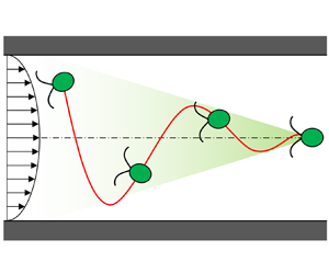
Figure 2(a) shows the trajectory of C. reinhardtii in the test section, which had a wavy trajectory with an amplitude of approximately 10  $\mathrm {\mu }$m and wavelength of approximately 700 $\mathrm {\mu }$m. The cell basically oriented against the background flow and tried to swim upstream. However, the background flow was too strong for the cell to swim upstream and the trajectory was directed toward a downstream side. We experimentally observed that the amplitude of wavy trajectories became smaller as cells moved downstream. As a result, the cells eventually accumulated around the channel centre, as observed by Barry et al. (Reference Barry, Rusconi, Guasto and Stocker2015). For the readers’ convenience, the trajectory and orientation of a cell in the channel is shown schematically in figure 2(b). Because gravity acts in the $z$-direction and the microscope illumination also comes from the $z$-direction, we can exclude any effect of gravitaxis and phototaxis on behaviours along the horizontal $x\text{--}y$ plane. Hence, the observed centreline accumulation might be induced by hydrodynamics, which will be further investigated in the following sections.

Figure 2. Migration of C. reinhardtii to the channel centre. (a) A sample trajectory of C. reinhardtii in the channel (scale bar  $= 50\ \mathrm {\mu }$m). White and yellow arrows indicate the directions of flow and trajectory, respectively. (b) Schematic diagram of the trajectory and orientation of the cell in the channel. (c) Amplitude of the trajectories of motile cells at different $x$ positions. Here, $n$ is the number of measurements. ( $^{**}{p} < 0.01$; Mann–Whitney U test with Bonferroni correction). (d) The amplitude of the trajectories of non-motile cells at different $x$ positions. ( $^{*}{p} < 0.05$; n.s.: non-significant).
Given that observing a very long trajectory can be difficult using a microscope, we measured the amplitude of the wavy trajectories at different positions in the test section, as shown in figure 2(c). The amplitude was significantly reduced as the cells flowed downstream. We found statistical significance of  $p < 0.01$ by using the Mann–Whitney U test with Bonferroni correction. The results clearly illustrated the migration of C. reinhardtii to the channel centre. To clarify the effect of cell motility on migration, we performed another experiment using non-motile cells, in which the cells were lightly fixed with glutaraldehyde. The results using the non-motile cells are shown in figure 2(d); notably, the non-motile cells showed no migration, thus indicating that cell motility was essential to induce migration.
C. reinhardtii in the test section also exhibited rheotaxis, as shown in figure 3. The cell changed its orientation along the wavy trajectory, as shown in figure 3(a), which is similar to figure 2(b). The rheotactic behaviour is confirmed in supplementary movie 1. In the movie, we also see unsteady swimming of C. reinhardtii, in which the cell oscillated back and forth owing to the effective and recovery strokes. To clarify the effect of cell motility on rheotaxis, we again performed another experiment using non-motile cells. The results using the non-motile cells are shown in figure 3(b). We see that the trajectory of a non-motile cell drew a straight path and the cell rotated like a passive rigid particle. These results indicated that cell motility was essential to induce rheotaxis. We defined the orientation angle  $\theta$ relative to the flow direction, as shown in figure 2(c), where $\theta = 0$ indicates the flow direction and $\theta = {\rm \pi}$ indicates the upstream direction. We see from figure 2(d) that most of the cells at $x = 10$ mm oriented against the flow, which clearly demonstrated rheotaxis of C. reinhardtii in channel flow.

Figure 3. Orientation of C. reinhardtii showing rheotaxis. (a) Sequential images of a sample motile cell in the channel. White arrow indicates the flow direction, yellow arrow indicates the direction of trajectory and black arrows indicate the orientations of cells (see also supplementary movie 1 available at https://doi.org/10.1017/jfm.2021.921). (b) Sequential images of a sample non-motile cell in the channel. (c) Definition of the orientation angle  $\theta$. Here, $\theta = {\rm \pi}$ indicates the direction against the flow. (d) Probability density of the orientation angle of cells at $x = 10$ mm ( $n = 300, N = 25$, where $n$ is the number of measurements and $N$ is the number of cells).
According to Polin et al. (Reference Polin2009), the time scale for C. reinhardtii to change its swimming direction is approximately 11.2 s. In the present study, it took approximately 40 s for C. reinhardtii to pass through the test section of 20 mm. Thus, we expected a few orientation changes of C. reinhardtii in the test section. We see that the results of figure 2(c) did not converge to 0 amplitude even at 20 mm, which may have be induced by the stochastic effect. This result also indicated that cells in the present study tended to orient against the flow even with the stochastic effect. This was probably because the time scale of rheotaxis (a couple of seconds) was much shorter than that of orientation change (11.2 s), and cells could direct against the flow during the straight swimming between orientation changes. In the orientation measurement, cells stayed in the field of view for approximately 0.4 s. Hence, we rarely observed the orientation change during the measurement.
3. Simulation using the boundary element method
Next, to clarify whether the observed rheotaxis and migration can be induced by physical forces or not, we performed a numerical simulation of swimming C. reinhardtii using the boundary element method (BEM). This step is important to exclude the unknown biological responses of cells, such as flagellar beat modification in response to the surrounding flow.
3.1. Basic equations and numerical methods
The basic equations and numerical methods employed in the BEM were similar to those used in our previous studies (Ito, Omori & Ishikawa Reference Ito, Omori and Ishikawa2019; Kage et al. Reference Kage2020). Thus, we explain them only briefly here.
Let us assume that a model of Chlamydomonas reinhardtii is suspended freely in an incompressible Newtonian liquid with viscosity  $\mu$ and density $\rho$. Because the experiments were performed in a horizontal channel flow, the effect of gravity can be neglected. Hence, the density of the cell model was assumed to be equivalent to the surrounding fluid. Owing to the small size of C. reinhardtii, the inertia effect of fluid motions can be neglected. The flow field is thus governed by the Stokes equation, which can be expressed as a boundary integral equation. We also applied slender body theory (Tornberg & Shelley Reference Tornberg and Shelley2004) to flagellar motions, because the radius of the flagellum was sufficiently small compared with its length.
The velocity at point  $\boldsymbol {x}$ can be expressed as
 \begin{equation} \boldsymbol{u}(\boldsymbol{x}) = \boldsymbol{u}^\infty(\boldsymbol{x}) -\frac{1}{8 {\rm \pi}\mu} \int_{body} \boldsymbol{\mathsf{J}}(\boldsymbol{x}, \boldsymbol{y}) \boldsymbol{\cdot} \boldsymbol{q}(\boldsymbol{y}) \, \textrm{d} A(\boldsymbol{y}) + {SBT}(\boldsymbol{x}) , \end{equation}
where  $\boldsymbol {u}^\infty$ is the background velocity, $\boldsymbol {q}$ is the traction force and $A$ indicates the cell surface. The integral is taken over the cell body. SBT indicates the contribution of flagella calculated using slender body theory. Here, $\boldsymbol{\mathsf{J}}$ is the Green function, defined as
 \begin{equation} \boldsymbol{\mathsf{J}} = \frac{\boldsymbol{\mathsf{I}}}{r} + \frac{\boldsymbol{r} \boldsymbol{r}}{r^3}, \end{equation}
where  $\boldsymbol{\mathsf{I}}$ is the identity matrix, $\boldsymbol {r} = \boldsymbol {x} - \boldsymbol {y}$ and $r = | \boldsymbol {r} |$. The contribution of flagella can be calculated as
 \begin{equation} {SBT}(\boldsymbol{x}) =
\left\{ \begin{array}{@{}ll} \displaystyle-\dfrac{1}{8 {\rm \pi}
\mu} {\boldsymbol{\Lambda}}(\boldsymbol{x})
\boldsymbol{\cdot} \boldsymbol{f}(\boldsymbol{x})
-\dfrac{1}{8 {\rm \pi}\mu} \int_{fla} [ \boldsymbol{\mathsf{J}}(\boldsymbol{x}, \boldsymbol{y}) \boldsymbol{\cdot}
\boldsymbol{f}(\boldsymbol{y}) \\ \quad - \boldsymbol{\mathsf{K}}(\boldsymbol{x}, \boldsymbol{y}) \boldsymbol{\cdot}
\boldsymbol{f}(\boldsymbol{x}) ] \, \textrm{d}
l(\boldsymbol{y}) & \mbox{when } \boldsymbol{x} \in \mbox{
flagella}, \\ \displaystyle-\dfrac{1}{8 {\rm \pi}\mu}
\int_{fla} [ \boldsymbol{\mathsf{J}}(\boldsymbol{x},
\boldsymbol{y}) + \boldsymbol{\mathsf{W}}(\boldsymbol{x},
\boldsymbol{y}) ] \boldsymbol{\cdot}
\boldsymbol{f}(\boldsymbol{y}) \, \textrm{d}
l(\boldsymbol{y}) & \mbox{otherwise},
\end{array} \right. \end{equation}
\begin{equation} {SBT}(\boldsymbol{x}) =
\left\{ \begin{array}{@{}ll} \displaystyle-\dfrac{1}{8 {\rm \pi}
\mu} {\boldsymbol{\Lambda}}(\boldsymbol{x})
\boldsymbol{\cdot} \boldsymbol{f}(\boldsymbol{x})
-\dfrac{1}{8 {\rm \pi}\mu} \int_{fla} [ \boldsymbol{\mathsf{J}}(\boldsymbol{x}, \boldsymbol{y}) \boldsymbol{\cdot}
\boldsymbol{f}(\boldsymbol{y}) \\ \quad - \boldsymbol{\mathsf{K}}(\boldsymbol{x}, \boldsymbol{y}) \boldsymbol{\cdot}
\boldsymbol{f}(\boldsymbol{x}) ] \, \textrm{d}
l(\boldsymbol{y}) & \mbox{when } \boldsymbol{x} \in \mbox{
flagella}, \\ \displaystyle-\dfrac{1}{8 {\rm \pi}\mu}
\int_{fla} [ \boldsymbol{\mathsf{J}}(\boldsymbol{x},
\boldsymbol{y}) + \boldsymbol{\mathsf{W}}(\boldsymbol{x},
\boldsymbol{y}) ] \boldsymbol{\cdot}
\boldsymbol{f}(\boldsymbol{y}) \, \textrm{d}
l(\boldsymbol{y}) & \mbox{otherwise},
\end{array} \right. \end{equation}
where  $\boldsymbol {f}$ is the viscous force per unit length acting on the flagella. The integral is taken along the flagella length of $L$. Here, ${{\boldsymbol{\Lambda}}}$ is the local operator given by
 \begin{equation} {{\boldsymbol{\Lambda}}}(\boldsymbol{x}) ={-} \ln{(\epsilon^2 e)} ( \boldsymbol{\mathsf{I}} + \boldsymbol{t}(\boldsymbol{x}) \boldsymbol{t}(\boldsymbol{x}) ) + 2( \boldsymbol{\mathsf{I}} - \boldsymbol{t}(\boldsymbol{x}) \boldsymbol{t}(\boldsymbol{x}) ) , \end{equation}
where  $\epsilon$ is the ratio between the radius and length of a flagellum, and $\boldsymbol {t}$ is the unit tangential vector of the flagellum. Additionally, $\boldsymbol{\mathsf{K}}$ is the integral operator given by
 \begin{equation} \boldsymbol{\mathsf{K}}(\boldsymbol{x}) = ( \boldsymbol{\mathsf{I}} + \boldsymbol{t}(\boldsymbol{x}) \boldsymbol{t}(\boldsymbol{x}) ) / | s(\boldsymbol{x}) - s(\boldsymbol{y}) | , \end{equation}
where  $s \in [0, L]$ is the arclength of the flagellum. Finally, $\boldsymbol{\mathsf{W}}$ is given by
 \begin{equation} \boldsymbol{\mathsf{W}} = \frac{(\epsilon L)^2}{2} \left[ \frac{\boldsymbol{\mathsf{I}}}{r^3} -3 \frac{\boldsymbol{rr}}{r^3} \right]. \end{equation}
Force-free and torque-free conditions of C. reinhardtii are given as
 $$\begin{gather} \boldsymbol{F} = \int_{body} \boldsymbol{q} \, \textrm{d} A + \int_{fla} \boldsymbol{f} \, \textrm{d} l = 0 , \end{gather}$$
 $$\begin{gather}\boldsymbol{T} = \int_{body} \boldsymbol{q} \wedge (\boldsymbol{x} - \boldsymbol{x}_c) \, \textrm{d} A + \int_{fla} \boldsymbol{f} \wedge (\boldsymbol{x} - \boldsymbol{x}_c) \, \textrm{d} l = 0 , \end{gather}$$
where  $\boldsymbol {x}_c$ is the geometric centre of the cell body.
To express the time-dependent flagellar beat, waveforms were extracted from experimental recordings (Kage et al. Reference Kage2020). In a two-dimensional image from an experimental movie, the material points of the centreline of the flagellum were tracked manually and interpolated in time and space using a cubic spline. Figure 4(a) shows the flagellar beat forms used in this study. Once the waveform during one period has been measured, we can calculate the flagellar velocity  $\boldsymbol {u}_{fla}$ with respect to the body frame. This prescribed flagellar velocity is given as the boundary condition of flagellar motion. Considering the no-slip condition, the velocity at the flagellar material point can be expressed as
 \begin{equation} \boldsymbol{u}(\boldsymbol{x}) = \boldsymbol{U} + {\boldsymbol \varOmega} \wedge (\boldsymbol{x} - \boldsymbol{x}_c) + \boldsymbol{u}_{fla} , \end{equation}
where  $\boldsymbol {U}$ and ${\boldsymbol \varOmega }$ are the translational and rotational velocities of the cell, respectively. We then solve the following resistance problem with respect to unknown variables $\boldsymbol {q}, \boldsymbol {f}, \boldsymbol {U}, {\boldsymbol \varOmega }$ (Ishikawa et al. Reference Ishikawa, Simmonds and Pedley2006),
 \begin{equation}
\left[\begin{array}{cc@{\hskip-2.2pc}c@{\hskip-2.5pc}|c} ~ & ~ & ~ & ~ \\ ~ & \mathcal{A}
& ~ & -\mathcal{B} \\ ~ & ~ & ~ & ~ \\ ~ & &\mbox{--------------------}~ & ~\\
& \mathcal{C} & ~ &
0 \end{array}\right] \left\{ \begin{array}{@{}c@{}}
\boldsymbol{q} \\ ~ \\ \boldsymbol{f} \\ \mbox{-----------} \\ \boldsymbol{U},
\boldsymbol{\varOmega} \end{array} \right\} = \left\{
\begin{array}{@{}c@{}} 0 \\ ~ \\ \boldsymbol{u}_{fla} -
\boldsymbol{u}^\infty \\ \mbox{----------------} \\ \boldsymbol{F}, \boldsymbol{T}
\end{array} \right\}. \end{equation}
\begin{equation}
\left[\begin{array}{cc@{\hskip-2.2pc}c@{\hskip-2.5pc}|c} ~ & ~ & ~ & ~ \\ ~ & \mathcal{A}
& ~ & -\mathcal{B} \\ ~ & ~ & ~ & ~ \\ ~ & &\mbox{--------------------}~ & ~\\
& \mathcal{C} & ~ &
0 \end{array}\right] \left\{ \begin{array}{@{}c@{}}
\boldsymbol{q} \\ ~ \\ \boldsymbol{f} \\ \mbox{-----------} \\ \boldsymbol{U},
\boldsymbol{\varOmega} \end{array} \right\} = \left\{
\begin{array}{@{}c@{}} 0 \\ ~ \\ \boldsymbol{u}_{fla} -
\boldsymbol{u}^\infty \\ \mbox{----------------} \\ \boldsymbol{F}, \boldsymbol{T}
\end{array} \right\}. \end{equation}

Figure 4. Simulation results obtained by the boundary element method (BEM). (a) Model C. reinhardtii. The cell body has length  $b$ and aspect ratio 1.2. The flagella of length $b$ generate the effective stroke (6–10) and recovery stroke (1–5). (b) Definition of the initial orientation angle $\phi _{ini}$ and the initial offset from the centreline $y_{ini}$. (c,d) Trajectories and orientation of cell models with various $\phi _{ini}$ ( $y_{ini} / b = -0.5$). (e,f) Trajectories and orientation of cell models with various $y_{ini}$ ( $\phi _{ini} / {\rm \pi}= 1.25$).
The cell body was assumed to be a prolate spheroid with an aspect ratio of 1.2, as shown in figure 4(a). The body length  $b$ and flagella length $L$ were set as 10 $\mathrm {\mu }$m. The flagellar radius was set as 100 nm, such that the ratio of the radius to the length of the flagellum was $\epsilon = 10^{-3}$. The cell surface was discretized by 1280 triangular elements and each flagellum was discretized by 100 line elements. The boundary integral equations were solved using the BEM, and the final simultaneous linear equations (3.10) were solved using a lower and upper factorization technique. The beat frequency was set to 50 Hz, corresponding to a beat period of $T = 0.02$ s, to mimic an actual cell. The time-marching process was carried out using a second-order Runge–Kutta method.
3.2. Simulation results
The cell model was placed in a parabolic flow, with an initial offset of  $y_{ini}$ from the centreline and with an initial angle of $\phi _{ini}$ relative to the $x$-axis, as shown in figure 4(b). The change in $x$ and $y$ positions over time with various $\phi _{ini}$ is shown in figure 4(c) ( $y_{ini} / b = -0.5$). In all cases, the cell eventually converged to the centreline, i.e. $y=0$. This migration tendency was equivalent to what we observed in the experiments. The change in orientation over time is shown in figure 4(d). In all cases, the cell eventually oriented against the flow, which was again consistent with our experimental observation. Although the cell basically oriented against the background flow and tried to swim upstream, the background flow was too strong for the cell to swim upstream. The trajectory was thus directed toward a downstream side, in the same manner with the experiment (cf. figure 2a).
The effect of  $y_{ini}$ is shown in figures 4(e) and 4(f) ( $\phi _{ini} / {\rm \pi}= 1.125$). In the range $y \le \pm 1.5 b = \pm 15\ \mathrm {\mu }$m, the cells again converged to the centreline as observed in the experiment. In all cases, the cell eventually oriented against the flow, which was again consistent with the experimental observation. These results illustrated that rheotaxis and migration were not influenced by the initial conditions.
To clarify the effect of cell motility, we also simulated the behaviours of non-motile cells in the channel. Flagella of non-motile cells were assumed to be rigid and their angles relative to the cell body were invariant with time. We here examined two kinds of flagella shapes, as shown in figure 5(a). The change in  $y$ position over time with the two kinds of flagella shapes is shown in figure 5(b) ( $y_{ini} / b = -0.5$, $\phi _{ini} / {\rm \pi}= 0.25$). In both cases, the cell drew a straight path and did not converge to the centreline. The change in orientation over time is shown in figure 5(c). The cell changed the orientation with periodic rotational velocity and did not show rheotaxis. These results clearly indicated that cell motility was essential for the migration and rheotaxis. The results may also be derived mathematically under Stokes flow conditions, given that drift and alignment do not appear for a body shape with plane symmetry (Kim & Karrila Reference Kim and Karrila1992; Ishimoto Reference Ishimoto2020).

Figure 5. Simulation results of non-motile cell models. (a) Rigid flagella shapes of non-motile cell models. (b,c) Trajectories and orientation of non-motile cells with the two kinds of flagella shapes ( $y_{ini}/b = -0.5$, $\phi _{ini} / {\rm \pi}= 0.25$).
Figure 6 shows the vector field of the orientation  $\phi$ and the $y$ position of the cell. The actual trajectory with $\phi _{ini} / {\rm \pi}= 1.125$ and $y_{ini} /b = -0.5$ is plotted as a black curve. We see that the vector field rotated in the counterclockwise direction, which meant that the cell swam across the channel centre and showed an overshoot. The arrows converged to the centre of the figure and there was a stable point at $\phi = {\rm \pi}$ and $y = 0$, in good agreement with the experiment. These results illustrated that the experimentally observed rheotaxis and migration could be reproduced by physical forces, without introducing any biological responses of cells.

Figure 6. Vector field of the orientation  $\phi$ and the $y$ position of the cell model. Each vector is obtained by averaging over one period of flagellar beat. The actual trajectory with $\phi _{ini} / {\rm \pi}= 1.125$ and $y_{ini} /b = -0.5$ is plotted as a black curve. Sample pathlines of the vector field are plotted as green curves for reference.
4. Analysis using a simple analytical model
Lastly, using a simple analytical model, we show that rheotaxis and migration can be explained by the interplay between cyclic swimming velocity and cyclic body deformation in the channel flow. For simplicity, let us assume that a model cell has a cyclic velocity  $U(t)$ and cyclic deformation with a Bretherton constant $B(t)$ given by
 $$\begin{gather} U(t) = U_s + U_c \sin(2 {\rm \pi}t / T) , \end{gather}$$
 $$\begin{gather}B(t) = B_s + B_c \sin(2 {\rm \pi}t / T + \lambda) , \end{gather}$$
where  $\lambda$ is the phase difference. The Bretherton constant is a dimensionless hydrodynamic measure of non-sphericity; i.e. $B=0$ for a sphere, $B > 0$ for a prolate object and $B < 0$ for an oblate object (Kim & Karrila Reference Kim and Karrila1992). The position $\boldsymbol {r}$ and orientation $\boldsymbol {e}$ of the cell are given by the following:
 $$\begin{gather} \frac{\textrm{d} \boldsymbol{r}}{\textrm{d} t} = U \boldsymbol{e} + \boldsymbol{u}^\infty , \end{gather}$$
 $$\begin{gather}\frac{\textrm{d} \boldsymbol{e}}{\textrm{d} t} = {\boldsymbol \varOmega}^\infty \wedge \boldsymbol{e} + B ( \boldsymbol{\mathsf{E}}^\infty \boldsymbol{\cdot} \boldsymbol{e} - \boldsymbol{\mathsf{E}}^\infty : \boldsymbol{ee}\ \boldsymbol{e} ) , \end{gather}$$
where  $\boldsymbol {u}^\infty$, ${\boldsymbol \varOmega }^\infty$ and $\boldsymbol{\mathsf{E}}^\infty$ are the velocity vector, vorticity vector and rate of the strain tensor of the background parabolic flow, respectively. The effect of wall boundary is omitted for simplicity.
4.1. Behaviours of the simple model swimmer
To determine the minimal requirements to induce rheotaxis and migration, we first consider a constant velocity swimmer ( $U_s \neq 0$ and $U_c = 0$) with cyclic deformation ( $B_c \neq 0$). As an example, we show the time change of the $y$-position under the condition $U_s T/L = B_c = 1$ and $U_c = B_s = 0$ in figure 7(a). Although the $y$-position oscillated considerably over time, its time-averaged value did not drift up to $t/T = 1000$. We did not observe migration nor rheotaxis in this case. We used many other parameter sets for a constant velocity swimmer; however, none of them showed migration nor rheotaxis.

Figure 7. Results of the simple analytical model for a constant velocity swimmer and a steady-shape swimmer. Time change of the  $y$-position for (a) the constant velocity swimmer with $U_s T/L = B_c = 1$ and $U_c = B_s = 0$, and (b) the steady-shape swimmer with $U_c T/L = 1$ and $U_s = B_s = B_c = 0$. The colour band indicates the maximum and minimum values owing to the cyclic motion.
We also consider a steady-shape swimmer ( $B_c = 0$) with a cyclic velocity ( $U_c \neq 0$). As an example, we show the time change of the $y$-position under the condition of $U_c T/L = 1$ and $U_s = B_s = B_c = 0$ in figure 7(b). The $y$-position again oscillated considerably over time; however, its time-averaged value did not drift up to $t/T = 1000$. Migration and rheotaxis were not observed in this case either. We performed many other parameter sets for a steady-shape swimmer; however, none of them showed migration nor rheotaxis.
Mimicking C. reinhardtii by the simple analytical model is a challenging task. The shape of C. reinhardtii containing two flagella is far from a spheroid and the shape changes with time owing to the flagellar beat. In the simple analytical model, however, all of the shape effects are concentrated on the Bretherton constant  $B$. The shape effects appear only on the rotational velocity through $B$, as given by (4.4). Thus, in mimicking C. reinhardtii by the simple analytical model, we evaluated the Bretherton constant of C. reinhardtii. The Bretherton constant can be computationally evaluated from the rotational velocity of the C. reinhardtii model with a given flagella shape. We placed the C. reinhardtii model in planer elongational flow with a tilt angle and the value of $B$ was calculated from (4.4) using the rotational velocity. The time change of $B$ is shown in figure 8 together with the swimming velocity $U$. We observed large oscillation of $B$ and $U$ during one period. The time variation was caused by the effective and recovery strokes of the cell. The time-averaged value of $B$ was approximately 0.32, which was equivalent to a prolate spheroid with aspect ratio of approximately 1.4. We regarded $B = 0.32$ to represent C. reinhardtii in the following. The peak-to-peak phase difference was $\Delta t / T \approx 0.41$, which corresponded to $\lambda = 2 {\rm \pi}(1 - \Delta t / T) \approx 1.2 {\rm \pi}$.

Figure 8. Time change of the swimming velocity  $U$ and the Bretherton constant $B$ of the C. reinhardtii model shown in the left. The time-averaged value of $B$ is approximately 0.32. The peak-to-peak phase difference is indicated by $\Delta t / T (\approx 0.41)$, which corresponds to $\lambda \approx 1.2 {\rm \pi}$.
We then analysed the motion of a prolate spheroidal swimmer with steady shape with  $B_s = 0.32$ and $B_c = 0$. Figure 9 shows the time change of the $y$-position of a steady swimmer ( $U_s T/L = 1$ and $U_c = 0$) and an unsteady swimmer ( $U_s T/L = 0.5$ and $U_c T/L = 1$). We again observed that the time-averaged value of $y$ did not drift up to $t/T = 1000$. We also did not observe rheotaxis in this case. Hence, the unsteady velocity alone was not sufficient to induce the migration nor rheotaxis. We note that the motion of a prolate spheroidal swimmer in Poiseuille flow was also investigated analytically and experimentally by Junot et al. (Reference Junot2019). However, the swimmers did not migrate to the channel centre, which is consistent with our study.

Figure 9. Results of the simple analytical model for a prolate spheroidal swimmer with the steady shape of  $B_s = 0.32$ and $B_c = 0$. Time change of the $y$-position for (a) the constant velocity swimmer with $U_s T/L = 1$ and $U_c = 0$, and (b) the unsteady velocity swimmer with $U_s T/L = 0.5$ and $U_c T/L = 1$. The colour band indicates the maximum and minimum values owing to the cyclic motion.
In contrast, both rheotaxis and migration were evident when the velocity and deformation were cyclic ( $U_c \neq 0$ and $B_c \neq 0$). Figure 10 shows the time change of the $y$-position and orientation of a cyclic swimmer with $U_s T/L = 0.5$, $U_c T/L = 1$, $B_s = 0.32$ and $B_c = 0.3$. This setting was similar to the C. reinhardtii model shown in figure 8. In figure 10, the swimmer was initially placed at $y/b = 0.25$ with orientation $\phi = 0.25 {\rm \pi}$. When $t/T \le 500$, the swimmer tumbled owing to the background vorticity and the orientation oscillated with the amplitude of ${\rm \pi}$. Meanwhile, the swimmer gradually migrated to the centreline, and eventually showed migration and rheotaxis. These results clearly illustrated that both cyclic velocity and cyclic body deformation were essential to induce migration and rheotaxis. Notably, swimmers did not show rheotaxis and migration in simple shear flow owing to the symmetry of the problem. Therefore, three ingredients, a cyclic swimming velocity, cyclic body deformation and a parabolic velocity profile, were necessary to induce rheotaxis and migration.

Figure 10. Results of the simple analytical model for a swimmer with cyclic body deformation and cyclic velocity ( $U_s T/L = 0.5$, $U_c T/L = 1$, $B_s = 0.32$ and $B_c = 0.3$). The swimmer is placed initially at $y/b = 0.25$ with orientation $\phi = 0.25 {\rm \pi}$. (a) Time change of the $y$-position and (b) time change of the orientation. The colour band indicates the maximum and minimum values owing to the cyclic motion.
4.2. Phase diagram of the swimming behaviours
To generalize the mechanism of rheotaxis and migration, we further simplify the problem settings. Figures 11(a) and 11(b) show the change in the  $y$ position of an oscillator over time ( $U_c T/L = B_c = 1$ and $U_s = B_s = 0$), as well as that of an unsteady swimmer ( $U_c T/L = B_c = 1$, $U_s T/L = 0.5$ and $B_s = 0$) in the low- and high-shear-rate regimes. The phase difference $\lambda$ was set as $1.2 {\rm \pi}$, which mimicked $\lambda \approx 1.2 {\rm \pi}$ of C. reinhardtii (cf. figure 8). By performing many trial simulations with different parabolic velocity profiles, we found that the migration tendency was strongly dependent on the dimension-free shear rate at the initial position $T \dot {\gamma }_{ini}$ of the object. When $T \dot {\gamma }_{ini}$ was large, the swimmer tended to migrate away from the centreline, where the shear rate was higher. Thus, the swimmer continuously migrated away from the centreline. When $T \dot {\gamma }_{ini}$ was small, however, the swimmer tended to migrate towards the centreline, where the shear rate was lower. Thus, the swimmer continuously migrated towards the centreline. By considering such tendencies, the dimension-free shear rate $T \dot {\gamma }_{ini}$ was taken as the vertical axis in figure 11 instead of $y$. We note that $\dot {\gamma } \propto y$ in parabolic flow; thus, the vertical axis can still be regarded as the $y$-axis, with $\dot {\gamma } = 0$ as the centreline of the channel.

Figure 11. Results of the simple analytical model for an oscillator and an unsteady swimmer. (a,b) Time change of the  $y$-position of the oscillator ( $U_c T/L = B_c = 1$ and $U_s = B_s = 0$) and the unsteady swimmer ( $U_c T/L = B_c = 1$, $U_s T/L = 0.5$ and $B_s = 0$). The $y$-position is replaced by the shear rate $\dot {\gamma }$, where $y$ is proportional to $\dot {\gamma }$ in parabolic flow, and $\dot {\gamma } = 0$ indicates the centreline. Here, $T \dot {\gamma }_{ini}$ is set as 1 or 5 and $\lambda$ is $1.2 {\rm \pi}$. The colour band indicates the maximum and minimum values owing to the cyclic motion. (c) Phase diagram of the migration direction of the oscillator in $\dot {\gamma }_{ini} - \lambda$ space. Positive $N$ indicates migration away from the centreline, whereas negative $N$ indicates migration to the centreline. The conditions for A and B are indicated by white circles, and those of the experiment and BEM simulation are indicated by a black circle.
Both the oscillator and the unsteady swimmer migrated to the centreline in the low-shear-rate regime (figure 11a). The unsteady swimmer migrated much more rapidly than the oscillator. These results illustrated that the steady velocity  $U_s$ was not necessary for migration, but dramatically accelerated migration. Both the oscillator and swimmer in this case also showed rheotaxis, i.e. they eventually oriented against the flow. In the high-shear-rate regime (figure 11b), the unsteady swimmer can still migrate to the centreline, while the oscillator migrates away from it. Hence, the steady velocity $U_s$ qualitatively affected migration in the high-shear regime.
A phase diagram of the migration direction of the oscillator in  $\dot {\gamma }_{ini} - \lambda$ space is shown in figure 11(c). At each data point, four kinds of initial orientations ( $\phi _{ini} = 0, {\rm \pi}/2, {\rm \pi}$ and $3{\rm \pi} /2$) were examined. The score $N$ was calculated as $N = N_w - N_c$, where $N_w$ is the number of initial conditions showing migration away from the centreline and $N_c$ is that showing migration to the centreline. By definition, we have $-4 \le N \le 4$ and $N_w + N_c = 4$. A positive $N$ indicated migration away from the centreline, whereas a negative $N$ indicated migration to the centreline.
When  $T \dot {\gamma }_{ini} < 4$, i.e. in the low-shear-rate regime, the migration tendency qualitatively changed with the phase difference $\lambda$. The oscillator did not migrate when the phase difference was $\lambda = 0$ and ${\rm \pi}$. In the $0 < \lambda < {\rm \pi}/2$ regime, the oscillator migrated to the centreline with a final orientation of $\phi _f = 0$, i.e. was directed downstream. In the ${\rm \pi} < \lambda < 3{\rm \pi} /2$ regime, the oscillator again migrated to the centreline, but with a final orientation of $\phi _f = {\rm \pi}$, i.e. was directed upstream. In the other regimes, including the high-shear-rate one, the oscillator tended to migrate away from the centreline. Thus, migration and rheotaxis were simultaneously observed only in the regime $T \dot {\gamma }_{ini} < 4$ and ${\rm \pi} < \lambda < 3{\rm \pi} /2$. Actually, C. reinhardtii has $\lambda \approx 1.2 {\rm \pi}$; our experiment and the BEM simulations were performed with $T \dot {\gamma }_{ini} < 1.25$. These conditions were within the regime of migration and rheotaxis, thus confirming consistency.
5. Conclusions
In this study, we clarified the novel physical mechanism of rheotaxis and migration in channel flow, which appears when an unsteady swimmer shows a phase difference between body deformation and swimming velocity. In the case of an oscillator, the rheotaxis and migration appear when  $T \dot {\gamma }_{ini} \le 4$ (cf. figure 11c). Because the period of C. reinhardtii is $T = 0.02$ s, the condition corresponds to $\dot {\gamma }_{ini} \le 200$ s $^{-1}$. This condition is not considerably affected by the initial orientations of cells (cf. figure 11c). Moreover, the swimming velocity enhances the rheotaxis and migration, as shown in figure 11(a,b). Thus, the parameter range to show rheotaxis and migration should be expanded by introducing the swimming velocity. The shear rate of 200 s $^{-1}$ can be found in many practical settings, such as in a bioreactor and blood flow in a vessel.
The relaxation time of the rheotaxis and migration, in the case of C. reinhardtii, can be estimated as  $t/T \approx 100$ (cf. Figure 4). By inserting $T = 0.02$ s, the relaxation time can be estimated as 2 s. This time scale tends to be shorter than that of gravitaxis, as the typical rotational velocity of gravitaxis is approximately 0.1 rad s $^{-1}$ (Kage et al. Reference Kage2020). The time scale of phototaxis is approximately 2 s (Garcia et al. Reference Garcia, Rafai and Peyla2013; Jibuti et al. Reference Jibuti2014), which is of the same order. Therefore, the present rheotaxis and migration would be superimposed on the conventional gravitaxis and phototaxis with a similar magnitude. Especially when the channel is horizontal and the illumination is homogeneous, the present mechanism should be the main driver of rheotaxis and migration.
The proposed mechanism is expected to apply to other microswimmer types. For example, mixotrophic species of haptophytes Prymnesium parvum have two flagella moving with a ciliary beat (Dölger et al. Reference Dölger2017). As a result, it changes its swimming velocity and body shape in a cyclic manner. An active amoeboid swimmer (Wu et al. Reference Wu2015, Reference Wu2016) and Golestanian's three-bead swimmer model (Golestanian & Ajdari Reference Golestanian and Ajdari2008) also show cyclic changes in swimming velocity and body shape. Thus, these swimmers should exhibit migration and rheotaxis in channel flow.
In nature, such unsteady cells can capture the main stream of the background flow and move downstream faster than steady cells. The present migration mechanism is in accordance with the shear rate gradient and may play a role in more complex flow fields, such as turbulence. We note that migration may arise from a combination of deterministic and stochastic mechanisms in the generic case, and that an effort needs to be made to assess their relative magnitudes in the future. The present migration mechanism also suggests that cells with similar beat patterns can join together via the migration mechanism, which may be biologically advantageous for mating. The migration tendency can also be used for cell sorting and separation in engineering applications. The knowledge obtained in this study improves our understanding of the behaviours of unsteady microswimmers in nature and engineering.
Supplementary movie
Supplementary movie is available at https://doi.org/10.1017/jfm.2021.921.
Funding
This study is supported by JSPS KAKENHI Nos. 18K18354 (T.O.), 19H02059 (K.K.), 21H05306 (K.K.), 17H00853 (T.I.), 21H04999 (T.I.), 21H05308 (T.I.). K.K. is also supported by JST FOREST No. JPMJFR2024. T.O. is also supported by JST PRESTO JPMJPR2142.
Declaration of interests
The authors report no conflict of interest.


 Open access