


1. Introduction
Howard Brenner has made numerous seminal contributions to the field of fluid dynamics. His early publications on low Reynolds number hydrodynamics were transformative, converting what was once regarded as a mainly academic and dull topic into the vibrant field of microfluidics (Acrivos Reference Acrivos2014). Understanding particle behaviour in the regime of low Reynolds numbers, where viscous forces dominate, is fundamentally important in various domains involving single particle dynamics, such as microswimmers, and in studies of particle suspensions and rheology. The geometry of a particle significantly affects its dynamics, making the development of theoretical techniques to study arbitrary and irregular geometries in Stokes flow a necessity.
Brenner has developed analytical approaches to address arbitrary geometries (Brenner Reference Brenner1963, Reference Brenner1964b,Reference Brennerc,Reference Brennerd, Reference Brenner1966). In one of his works (Brenner Reference Brenner1964a), which is the focus of our paper, he used an asymptotic expansion of the velocity field to address the problems of slightly deformed spheres within a perturbative framework. The literature citing this seminal work reveals that its significance, particularly in the field of microswimmers, has not yet been fully recognized. Most analytical and semi-analytical studies within this domain focus on spheres, spheroids, slender bodies or nearly spherical particles with slight deformations. Revisiting his formalism to evaluate its validity range and extend its application to more significantly deformed spheres would enable researchers to distinctly observe the effects of various orders of perturbation on particle motion, thus opening up the exploration of a broader class of microswimmer geometries with insights into microswimmer dynamics.
Brenner's method (Brenner Reference Brenner1964a) defines the surface of a deformed sphere  $\mathbb {S}$ as a radial deformation of the surface $\mathbb {S}_0$ of a hypothetical reference sphere, using a deformation shape function $\xi$ and a deformation amplitude $\delta$. The process of solving the flow field around the slightly deformed sphere consists of two mapping steps: the first mapping, $\boldsymbol {u}(\boldsymbol {r}_{S}) \mapsto \boldsymbol {u}(\boldsymbol {r}_{0})$, translates the velocity field from the surface of the deformed sphere, $\mathbb {S}$, to that of the reference sphere, $\mathbb {S}_0$. Then, using the second mapping, $\boldsymbol {u}(\boldsymbol {r}_0) \mapsto \boldsymbol {u}(\boldsymbol {r})$, it extends from $\mathbb {S}_0$ to any point in the fluid, $\boldsymbol {r}$, using Lamb's general solution of the Stokes equation (Lamb Reference Lamb1932).
The first mapping  $\boldsymbol {u}(\boldsymbol {r}_{S}) \mapsto \boldsymbol {u}(\boldsymbol {r}_{0})$ is achieved for different orders of deformation amplitude $\delta$ through the coupling of the asymptotic expansion of the velocity field in terms of $\delta$ with the Taylor expansion of the velocity field over the deformed sphere about the surface of the reference sphere. The complexity in the calculations stems from the need to calculate progressively higher-order radial derivatives due to the Taylor expansion in the first mapping and to successively apply the second mapping and gradient operations in Lamb's general solution for Stokes flow around the reference sphere for each order of perturbation. Therefore, while his elegant framework is mathematically rigorous and can, in principle, handle higher orders of perturbations, the analytical calculations become rapidly more complicated as one goes beyond the first order, making it practically difficult to obtain higher-order terms.
In this paper, we assess the range of validity of Brenner's first mapping, specifically using the hydrodynamic radius as the measure of Stokes resistance, and demonstrate its applicability to highly deformed spheres. By leveraging spectral modes (Nabil et al. Reference Nabil, Nabavizadeh, Lammert and Nourhani2022), we transform Brenner's first mapping from its differential form into simple matrix-based expressions by adopting a spectral expansion method instead of using Lamb's general solution for the second mapping. This resulting matrix-based framework streamlines the computational process for each perturbation order. We can apply the first mapping up to the desired perturbation order and use the resulting asymptotic sum of the expansion coefficients collectively for the second mapping. This approach eliminates the need to apply the second mapping independently for each perturbation order. Moreover, the hydrodynamic radius is proportional to one of the expansion coefficients, allowing for straightforward computation to track the convergence and the validity range of the first mapping. Our findings demonstrate that Brenner's first mapping can accommodate highly deformed geometries, extending beyond the linear term for slightly deformed spheres in the asymptotic expansion.
2. Basis and development of the method
This section develops the matrix-based framework for studying the range of the validity of Brenner's first mapping for obtaining the Stokes resistance of an axisymmetric deformed sphere in an axisymmetric flow. We begin by reviewing the mathematical formalism of his method that we discussed in the introduction. Afterwards, we will combine the first mapping in differential formal with spectral formalism for axisymmetric Stokes flow to reformulate the mapping in terms of matrix algebra and obtain an expression for hydrodynamic radius of the deformed sphere in terms of spectral expansion coefficients.
2.1. Problem formulation
The axisymmetric particle's geometry results from the radial deformation of a reference sphere  $\mathbb {S}_0$ of radius $r_0$ centred at the origin. In spherical coordinates the surface $\mathbb {S}$ of the axisymmetric particle is given by
 \begin{equation} {\boldsymbol{r}}_{S}(\theta) = {\boldsymbol{r}}_0[1 + \delta \xi(\theta)], \end{equation}
where  $\xi$ represents the shape function, and $\delta$ denotes the amplitude of the deformation. The particle moves along its symmetry axis through an incompressible Newtonian fluid with viscosity $\mu$, under conditions of low Reynolds number hydrodynamics. The far-field vanishing velocity field is governed by the Stokes and continuity equations
 \begin{equation} \mu \nabla^2 {\boldsymbol{u}} = \boldsymbol{\nabla} p, \quad \boldsymbol{\nabla}\boldsymbol{\cdot} {\boldsymbol{u}} = 0. \end{equation}
We will construct a formal expansion of the velocity field around the particle in powers of the deformation amplitude  $\delta$, as
 \begin{equation} {\boldsymbol{u}}({\boldsymbol{r}}) \stackrel{F}= \sum_{k=0} \delta^k {\boldsymbol{u}}^{(k)}({\boldsymbol{r}}). \end{equation}
The ‘ $F$’ atop the equals sign is a reminder that this is a formal expansion and there is no a priori reason to assume that it converges. Indeed, our calculations strongly suggest that it does not. Practical computations must be cut off at some maximum order, $k_{max}$, of perturbation theory, anyway, and the question remains of how good results can be obtained as $\delta$ and $k_{max}$ vary. In the following, we adhere to the following conventions: $k$ and $q$ are reserved for denoting orders of perturbation, $k_{max}$ is our maximum computational cutoff and other formal expansions like (2.3) will be written with an ordinary equals sign. Typically, the convergence of the asymptotic $\delta$-expansion (2.3) remains ambiguous, as noted in Brenner (Reference Brenner1964a). However, the more pertinent question is whether a limited number of terms can provide a physically valid response.
2.2. Brenner's mapping steps
This section reviews the differential form expression for Brenner's first mapping (Brenner Reference Brenner1964a). Utilizing the representation (2.1) for the surface  $\mathbb {S}$ of the radially deformed sphere in terms of the surface $\mathbb {S}_0$ of the reference sphere, the Taylor expansion of the velocity field about the reference sphere $\mathbb {S}_0$ yields ${\boldsymbol {u}}({\boldsymbol {r}}_{S}) = {\boldsymbol {u}}({\boldsymbol {r}}_0) + \sum _{q=1}^\infty \delta ^q (q!)^{-1}(r_0\xi )^q \partial _r^q {\boldsymbol {u}}|_{{\boldsymbol {r}}={\boldsymbol {r}}_0}$. Combining the asymptotic expansion (2.3) with the Taylor expansion and upon rearranging, we obtain the velocity field over the surface of the reference sphere for each order of perturbation, and thus Brenner's mapping
 \begin{equation} \boldsymbol{u}(\boldsymbol{r}_{S})\mapsto\boldsymbol{u}(\boldsymbol{r}_{0}): \begin{cases}{\boldsymbol{u}}^{(0)}({\boldsymbol{r}}_0) = {\boldsymbol{u}}^{(0)}({\boldsymbol{r}}_{\!_S}),\qquad\qquad\qquad\qquad\qquad\qquad\qquad\qquad\\ {\boldsymbol{u}}^{(k)}({\boldsymbol{r}}_0) = {\boldsymbol{u}}^{(k)}({\boldsymbol{r}}_{\!_S}) - \sum\limits_{q=1}^k \left.\dfrac{(r_0\xi)^q}{q!} \dfrac{\partial^q {\boldsymbol{u}}^{(k-q)}}{\partial r^q}\right|_{r=r_0}\quad \text{for}\ k \geqslant 1. \end{cases} \end{equation}
The leading-order terms for the surface velocity field over the surfaces of the reference and the deformed spheres are equal. Assuming we have a framework to apply the second mapping,  $\boldsymbol {u}(\boldsymbol {r}_0) \mapsto \boldsymbol {u}(\boldsymbol {r})$, and we can solve for the velocity field around a sphere with an arbitrary surface velocity distribution, we can determine the leading-order velocity field ${\boldsymbol {u}}^{(0)}({\boldsymbol {r}})$ using (2.4a). This term will then be used in the radial derivative in (2.4b), along with the first-order term from the boundary condition ${\boldsymbol {u}}^{(1)}({\boldsymbol {r}}_{\!_S})$ on the deformed sphere, to obtain the first-order boundary condition ${\boldsymbol {u}}^{(1)}({\boldsymbol {r}}_0)$ on the reference sphere. From this, we solve to obtain ${\boldsymbol {u}}^{(1)}({\boldsymbol {r}})$. This process continues iteratively to obtain higher orders.
Thus, for each increment in the order of perturbation in (2.4b), we have to solve for the flow fields by applying the second mapping to all the lower orders. Therefore, one of our goals will be to computationally decouple the first mapping from the second mapping, eliminating the need to apply the second mapping independently for each perturbation order. This ensures that the framework of the first mapping is self-sufficient, which will aid in examining its range of its validity.
2.3. Spectral method applied to Brenner's mapping
In this section, we combine Brenner's mapping (2.4) with the spectral method (Nabil et al. Reference Nabil, Nabavizadeh, Lammert and Nourhani2022) for axisymmetric flow to develop a matrix-based framework for the first mapping. Within the spectral method, the velocity field is expanded in terms of axisymmetric spectral modes  ${\boldsymbol {u}}_{\ell }^{[\alpha ]}({\boldsymbol {r}})$: the biharmonic mode ( $\nabla ^2\nabla ^2{\boldsymbol {u}}^{[1]}_\ell =0, \nabla ^2{\boldsymbol {u}}^{[1]}_\ell \neq 0$) and the pressure-free harmonic mode ( $\nabla ^2{\boldsymbol {u}}^{[2]}_\ell = 0$), both of which satisfy the Stokes and continuity equations (2.2a,b). Using the inner product $\langle {\boldsymbol {f}} | {\boldsymbol {g}} \rangle = \int _0^{{\rm \pi} } {\boldsymbol {f}}\boldsymbol {\cdot }{\boldsymbol {g}} \sin \theta \,{\rm d}\theta$ between two axisymmetric vectorial functions defined over the sphere surface, the Stokes velocity field around a sphere is
 \begin{equation} {\boldsymbol{u}}({\boldsymbol{r}}) = \sum_{\alpha=1}^2 \sum_{\ell=1}^{\ell_{max}} \left\langle {\boldsymbol{D}}_{\ell}^{[\alpha]} \middle| {\boldsymbol{u}} ({\boldsymbol{r}}_0)\right\rangle {\boldsymbol{u}}_{\ell}^{[\alpha]}({\boldsymbol{r}}) ,\end{equation}
where the boundary condition  ${\boldsymbol {u}} ({\boldsymbol {r}}_0)$ represents the arbitrary velocity field over the sphere's surface. Dual fields ${\boldsymbol {D}}_\ell ^{[\alpha ]}$ defined over the sphere's surface satisfy the orthogonality relation $\langle {\boldsymbol {D}}_{\ell _1}^{[\alpha _1]} | {\boldsymbol {u}}_{\ell _2}^{[\alpha _2]} ({\boldsymbol {r}}_0)\rangle = \delta _{\ell _1\ell _2}\delta _{\alpha _1\alpha _2}$.
The summation over  $\ell$ theoretically has no upper bound; however, for calculations, we need to set a cutoff value $\ell _{max}$. The explicit expressions for the axisymmetric spectral modes and their corresponding dual vectors are presented in (3.1) in § 3, where we discuss the implementation of the method. The modes are homogeneous in the radial coordinate
 \begin{equation} {\boldsymbol{u}}^{[\alpha]}_\ell \propto r^{{-}n^{[\alpha]}_\ell}, \quad n^{[\alpha]}_\ell = \ell \delta_{1,\alpha} + (\ell+2) \delta_{2,\alpha}. \end{equation}
 The linearity and simplicity of the spectral expansion (2.5) provide us with a basis to reformulate the first mapping (2.4) into a set of matrix-based calculations that can be easily implemented numerically, as we elaborate below. Taking the inner product of both sides of the equations in the mapping (2.4) with  ${\boldsymbol {D}}_{\ell }^{[\alpha ]}$ for each perturbation order $k$ generates the terms
 \begin{equation} {\mathcal{A}}_{\ell}^{[\alpha] (k)} = \left\langle {\boldsymbol{D}}_{\ell}^{[\alpha]} \middle| {\boldsymbol{u}}^{(k)} ({\boldsymbol{r}}_0)\right\rangle, \quad {\mathcal{S}}_\ell^{[\alpha] (k)} = \left\langle {\boldsymbol{D}}_{\ell}^{[\alpha]} \middle| {\boldsymbol{u}}^{(k)} ({\boldsymbol{r}}_{S}) \right\rangle, \end{equation}
where  ${\mathcal {S}}_{\ell }^{[\alpha ] (k)}$ encodes the boundary condition over the surface of the deformed sphere. We are interested in obtaining asymptotic expansion coefficients ${\mathcal {A}}_{\ell }^{[\alpha ] (k)}$ which provide us with the coefficients for the spectral expansion of the velocity field (2.5), that is,
 \begin{equation} \left\langle {\boldsymbol{D}}_{\ell}^{[\alpha]} \middle| {\boldsymbol{u}} ({\boldsymbol{r}}_0)\right\rangle =\sum_{k=0}^\infty \delta^k {\mathcal{A}}_{\ell}^{[\alpha] (k)}. \end{equation}
 Therefore, we are left with developing a framework to obtain the coefficients  ${\mathcal {A}}_{\ell }^{[\alpha ] (k)}$ in terms of the boundary condition coefficient ${\mathcal {S}}_{\ell }^{[\alpha ] (k)}$ using Brenner's first mapping (2.4). Taking inner products with a dual vector ${\boldsymbol {D}}_{\ell }^{[\alpha ]}$ in the mapping expression (2.4), and using
 \begin{equation} ({-}r_0)^q \partial_r^q {\boldsymbol{u}}^{[\alpha']}_{\ell'}|_{r=r_0} = \frac{(q + n^{[\alpha']}_{\ell'} - 1)!}{(n^{[\alpha']}_{\ell'}-1)!} {\boldsymbol{u}}^{[\alpha']}_{\ell'}({\boldsymbol{r}}_0), \end{equation}
along with the notations (2.7a,b) yields the reformulation of Brenner's first mapping within a matrix-based framework
 \begin{equation} {\boldsymbol{u}}({\boldsymbol{r}}_{S})\mapsto{\boldsymbol{u}}({\boldsymbol{r}}_{0}): \begin{cases} {\mathcal{A}}_\ell^{[\alpha](0)} = {\mathcal{S}}_\ell^{[\alpha](0)}, & \\ {\mathcal{A}}_\ell^{[\alpha](k)} = {\mathcal{S}}_\ell^{[\alpha](k)} - \sum\limits_{q=1}^k {\boldsymbol{\varXi}}^{[\alpha,\alpha'](q)}_{\ell,\ell'} {\mathcal{A}}_{\ell'}^{[\alpha'](k-q)} & \text{for}\ k \geqslant 1, \end{cases} \end{equation}
where the geometrical coefficients
 \begin{equation} {\boldsymbol{\varXi}}^{[\alpha,\alpha'](q)}_{\ell,\ell'} = ({-}1)^q \frac{(q + n^{[\alpha']}_{\ell'} - 1)!}{q! (n^{[\alpha']}_{\ell'}-1)!} \left\langle {\boldsymbol{D}}_{\ell}^{[\alpha]} \middle| \xi^q {\boldsymbol{u}}^{[\alpha']}_{\ell'} ({\boldsymbol{r}}_0) \right\rangle, \end{equation}
depend on the deformation function  $\xi$, and thus, are known. The exponents $n^{[\alpha ']}_{\ell '}$ are defined in (2.6a,b). The only unknowns in matrix-based mapping (2.10) are the coefficients ${\mathcal {A}}_\ell ^{[\alpha ](k)}$ that we aim to calculate in order. Hence, the knowledge of the boundary condition over the deformed sphere through the terms ${\mathcal {S}}_\ell ^{[\alpha ] (k)}$, as described in the mapping (2.10), provides a self-sufficient set of equations for obtaining the coefficients ${\mathcal {A}}_\ell ^{[\alpha ](k)}$ without the need to apply the second mapping as we increment the perturbation order. Effectively, after obtaining the spectral expansion coefficients (2.8) we automatically also obtain the velocity field (2.5) around an axisymmetric radially deformed sphere.
To find the Stokes resistance of the deformed sphere, consider the force exerted on the fluid by the particle moving along its symmetry axis  $\hat {\boldsymbol {e}}_{z} \equiv \frac {8}{3} {\boldsymbol {D}}_{1}^{[1]}$. It is given by $F_z = 6{\rm \pi} \mu r_0 \hat {\boldsymbol {e}}_{z} \boldsymbol {\cdot }\overline {{\boldsymbol {u}}({\boldsymbol {r}}_0)} = {8{\rm \pi} \mu r_0} \langle {\boldsymbol {D}}_{1}^{[1]} \mid {\boldsymbol {u}}({\boldsymbol {r}}_0) \rangle,$ where $\overline {{\boldsymbol {u}}({\boldsymbol {r}}_0)}$ is the average over the reference sphere. The Stokes resistance of the particle is characterized by the hydrodynamic radius $r_H = F_z/(6{\rm \pi} \mu )$, defined as the radius of a sphere with the same drag coefficient as the deformed spheres moving with velocity ${\boldsymbol {u}}({\boldsymbol {r}}_S) \equiv \hat {\boldsymbol {e}}_{z}$ along its symmetry axis. The ratio of the hydrodynamic radius to the radius of the reference sphere is
 \begin{equation} \frac{r_H}{r_0} = \frac{4}{3}\langle {\boldsymbol{D}}_{1}^{[1]} \mid {\boldsymbol{u}}({\boldsymbol{r}}_0) \rangle = \frac{4}{3} \sum_{k=1}^{k_{max}} \delta^k {\mathcal{A}}_{1}^{[1] (k)} . \end{equation}
We will determine the range of validity of Brenner's first mapping from a deformed sphere to a reference sphere in the matrix form (2.10) by calculating the hydrodynamic resistance and comparing the results with those of the direct spectral method calculations (Nabil et al. Reference Nabil, Nabavizadeh, Lammert and Nourhani2022).
3. Computational implementation
This section provides details on the implementation of the mapping (2.10) within a simple matrix-based framework. We use the following axisymmetric spectral modes and their corresponding dual vectors (Nabil et al. Reference Nabil, Nabavizadeh, Lammert and Nourhani2022):
 $$\begin{align} \ell \geqslant 1: &\quad {\boldsymbol{u}}_\ell^{[1]}({\boldsymbol{r}}) = \left(\frac{r_0}{r} \right)^{\ell}\left[ \ell(\ell+1) {\boldsymbol{P}}^{[1]}_\ell(\cos\theta) - (\ell-2){\boldsymbol{P}}^{[2]}_\ell(\cos\theta)\right], \end{align}$$
 $$\begin{align}&\quad {\boldsymbol{D}}_\ell^{[1]}(\cos\theta) = \frac{2\ell+1}{4 \ell(\ell+1)}\left[ \ell{\boldsymbol{P}}^{[1]}_\ell( \cos\theta) + {\boldsymbol{P}}^{[2]}_\ell(\cos\theta)\right], \end{align}$$
 $$\begin{align}\ell \geqslant 1: &\quad {\boldsymbol{u}}_\ell^{[2]}({\boldsymbol{r}}) = \left(\frac{r_0}{r} \right)^{\ell+2}\left[-(\ell+1) {\boldsymbol{P}}^{[1]}_\ell(\cos\theta) + {\boldsymbol{P}}^{[2]}_\ell(\cos\theta)\right], \end{align}$$
 $$\begin{align}&\quad {\boldsymbol{D}}_\ell^{[2]}(\cos\theta) = \frac{2\ell+1}{4(\ell+1)}\left[ (\ell-2){\boldsymbol{P}}^{[1]}_\ell(\cos\theta) + {\boldsymbol{P}}^{[2]}_\ell(\cos\theta)\right]. \end{align}$$
The orthogonal basis functions  ${\boldsymbol {P}}^{[1]}_\ell = \text {P}_\ell (\cos \theta )\hat {\boldsymbol {e}}_{r}$ and ${\boldsymbol {P}}^{[2]}_\ell = \text {P}_{\ell }^1(\cos \theta )\hat {\boldsymbol {e}}_{\theta }$ obey the orthogonality relation $\langle {\boldsymbol {P}}_{\ell _1}^{[\alpha _1]} | {\boldsymbol {P}}_{\ell _2}^{[\alpha _2]} \rangle = {2}/({2\ell _1+1}) [\delta _{1,\alpha _1} + \ell _1(\ell _1+1) \delta _{2,\alpha _1}] \delta _{\alpha _1\alpha _2}\delta _{\ell _1\ell _2}$, where $\text {P}_{\ell }^m$ is the associated Legendre polynomial of degree $\ell$ and order $m$, and $\hat {\boldsymbol {e}}_{r}$ and $\hat {\boldsymbol {e}}_{\theta }$ are unit vectors in the $r$ and $\theta$ directions, respectively.
By setting a finite value  $\ell _{max}$ for the upper bound of $\ell$ in the spectral expansion (2.5), we can treat the pair $(\alpha,\ell )$ as a compound index, which turns the spectral mapping expression (2.10) into matrix-based calculations
 \begin{equation} \boldsymbol{\mathcal{A}}^{(k)} = \boldsymbol{\mathcal{S}}^{(k)} - \sum_{q=1}^k {\boldsymbol{\varXi}}^{(q)} \boldsymbol{\mathcal{A}}^{(k-q)}, \end{equation}
where the explicit forms with  $1 \leqslant \ell, \ell ' \leqslant \ell _{max}$ are
 \begin{gather}
{\boldsymbol{\varXi}}^{(q)} = \left(\frac{\dfrac{({-}1)^q
(q + \ell' - 1)!}{q! (\ell'-1)!} {\left\langle
{\boldsymbol{D}}_{\ell}^{[1]} \middle| \xi^q
{\boldsymbol{u}}_{\ell'}^{[{1}]}({\boldsymbol{r}}_0)
\right\rangle}\,\bigg|\, \dfrac{({-}1)^q (q + \ell' +
1)!}{q! (\ell' + 1)!} {\left\langle
{\boldsymbol{D}}_{\ell}^{[{1}]} \middle| \xi^q
{\boldsymbol{u}}_{\ell'}^{[{2}]}({\boldsymbol{r}}_0)
\right\rangle}} {\dfrac{({-}1)^q (q + \ell' - 1)!}{q!
(\ell'-1)!} {\left\langle {\boldsymbol{D}}_{\ell}^{[{2}]}
\middle| \xi^q
{\boldsymbol{u}}_{\ell'}^{[{1}]}({\boldsymbol{r}}_0)
\right\rangle}\,\bigg|\, \dfrac{({-}1)^q (q + \ell' +
1)!}{q! (\ell' + 1)!} {\left\langle
{\boldsymbol{D}}_{\ell}^{[{2}]} \middle| \xi^q
{\boldsymbol{u}}_{\ell'}^{[{2}]}({\boldsymbol{r}}_0)
\right\rangle}} \right),\nonumber\\ \boldsymbol{\mathcal{A}}^{(k)} =
\left(\frac{\left\langle {\boldsymbol{D}}_{\ell}^{[1]}
\middle| {\boldsymbol{u}}^{(k)} ({\boldsymbol{r}}_0)
\right\rangle}{\left\langle {\boldsymbol{D}}_{\ell}^{[2]}
\middle| {\boldsymbol{u}}^{(k)}
({\boldsymbol{r}}_0)\right\rangle}\right),\quad
\boldsymbol{\mathcal{S}}^{(k)} = \left(\frac{\left\langle
{\boldsymbol{D}}_{\ell}^{[1]} \middle|
{\boldsymbol{u}}_s^{(k)} \right\rangle} { \left\langle
{\boldsymbol{D}}_{\ell}^{[2]} \middle|
{\boldsymbol{u}}_s^{(k)}\right\rangle}\right).
\end{gather}
\begin{gather}
{\boldsymbol{\varXi}}^{(q)} = \left(\frac{\dfrac{({-}1)^q
(q + \ell' - 1)!}{q! (\ell'-1)!} {\left\langle
{\boldsymbol{D}}_{\ell}^{[1]} \middle| \xi^q
{\boldsymbol{u}}_{\ell'}^{[{1}]}({\boldsymbol{r}}_0)
\right\rangle}\,\bigg|\, \dfrac{({-}1)^q (q + \ell' +
1)!}{q! (\ell' + 1)!} {\left\langle
{\boldsymbol{D}}_{\ell}^{[{1}]} \middle| \xi^q
{\boldsymbol{u}}_{\ell'}^{[{2}]}({\boldsymbol{r}}_0)
\right\rangle}} {\dfrac{({-}1)^q (q + \ell' - 1)!}{q!
(\ell'-1)!} {\left\langle {\boldsymbol{D}}_{\ell}^{[{2}]}
\middle| \xi^q
{\boldsymbol{u}}_{\ell'}^{[{1}]}({\boldsymbol{r}}_0)
\right\rangle}\,\bigg|\, \dfrac{({-}1)^q (q + \ell' +
1)!}{q! (\ell' + 1)!} {\left\langle
{\boldsymbol{D}}_{\ell}^{[{2}]} \middle| \xi^q
{\boldsymbol{u}}_{\ell'}^{[{2}]}({\boldsymbol{r}}_0)
\right\rangle}} \right),\nonumber\\ \boldsymbol{\mathcal{A}}^{(k)} =
\left(\frac{\left\langle {\boldsymbol{D}}_{\ell}^{[1]}
\middle| {\boldsymbol{u}}^{(k)} ({\boldsymbol{r}}_0)
\right\rangle}{\left\langle {\boldsymbol{D}}_{\ell}^{[2]}
\middle| {\boldsymbol{u}}^{(k)}
({\boldsymbol{r}}_0)\right\rangle}\right),\quad
\boldsymbol{\mathcal{S}}^{(k)} = \left(\frac{\left\langle
{\boldsymbol{D}}_{\ell}^{[1]} \middle|
{\boldsymbol{u}}_s^{(k)} \right\rangle} { \left\langle
{\boldsymbol{D}}_{\ell}^{[2]} \middle|
{\boldsymbol{u}}_s^{(k)}\right\rangle}\right).
\end{gather}
The elements can be evaluated by integrating over the polar angle  $\theta$. To the leading order, $\boldsymbol {\mathcal {A}}^{(0)} = \boldsymbol {\mathcal {S}}^{(0)}$, and we calculate $\boldsymbol {\mathcal {A}}^{(k)}$ for higher orders $k$ in terms of $\boldsymbol {\mathcal {S}}^{(k)}$, $\boldsymbol {\mathcal {A}}^{(q)}$ and the geometrical matrices $\boldsymbol {\varXi }^{(q)}$ for $q < k$.
For our analysis, we studied a family of geometries parametrized by  $(n, \delta )$, where $n$ is the degree of the Chebyshev polynomials of the first kind that defines the axisymmetric deformation function in (2.1)
 \begin{equation} \xi(\theta) = T_n(\cos\theta) = \cos n \theta, \end{equation}
whose powers can be expanded in terms of the Legendre polynomials of the first kind,  $\xi ^q(\theta ) = \sum _{\ell = 0}^{qn} C_\ell (n,q) \, P_{\ell }(\cos \theta ),$ with rational coefficients $C_{\ell }(n,q)\in \mathbb {Q}.$ Instead of direct integration, using this expansion turns the calculation of the $\langle {\boldsymbol {D}}_{\ell }^{[\alpha ]} \,|\, \xi ^q {\boldsymbol {u}}_{\ell '}^{[\alpha ']} ({\boldsymbol {r}}_0)\rangle$ into exact arithmetic by algebraic summations over the weighted sum of the terms
 $$\begin{gather} \left \langle {\boldsymbol{P}}_{\ell}^{[1]}\middle| P_{\ell''} {\boldsymbol{P}}_{\ell'}^{[1]}\right \rangle = 2\left (\begin{matrix} \ell & \ell'' & \ell'\\ 0 & 0 & 0 \end{matrix} \right)^{2}, \end{gather}$$
 $$\begin{gather}\left \langle {\boldsymbol{P}}_{\ell}^{[2]}\middle| P_{\ell''} {\boldsymbol{P}}_{\ell'}^{[2]}\right \rangle ={-}2\sqrt{\ell(\ell+1)\,\ell'(\ell'+1)} \left( \begin{matrix} \ell & \ell'' & \ell'\\ 0 & 0 & 0 \end{matrix} \right) \left(\begin{matrix} \ell & \ell'' & \ell'\\ -1 & 0 & 1 \end{matrix} \right), \end{gather}$$
where  $(\begin{smallmatrix} \ell & \ell '' & \ell ' \\ m & m'' & m' \end{smallmatrix})$ is the Wigner $3j$-symbol. The particle moves with velocity ${\boldsymbol {u}}({\boldsymbol {r}}_S) \equiv \hat {\boldsymbol {e}}_{z}$ for which ${\mathcal {S}}^{[1](0)}_1 = \frac {3}{4}$, ${\mathcal {S}}^{[2](0)}_1 = \frac {1}{4}$ and otherwise ${\mathcal {S}}^{[\alpha ](k)}_\ell = 0$.
4. Numerical results and comparison with direct spectral method
We explored a suite of axisymmetric radially deformed spheres with parameters  $n = 2, 3, \dots, 9$ for the deformation function (3.4). We studied the convergence of the hydrodynamic radius based on the cutoff value $\ell _{max}$ for the spectral expansion of the velocity (2.5) that appears in calculations (3.2) and (3.3). The convergence is monitored by tracking the value of the first element of $\boldsymbol {\mathcal {A}}^{(k)}$, that is, ${\mathcal {A}}^{[1](k)}_1$, for each perturbation order $k$, which is proportional to the corresponding hydrodynamic radius (2.12) for that order, and thus is of primary interest. In practice, we found that, for each order of perturbation, the term ${\mathcal {A}}^{[1](k)}_1$ typically begins to converge for $\ell _{max}$ in the range of approximately 10 to 20.
In terms of the asymptotic expansion, we are interested in the first few terms that yield physically reasonable values for  $r_H/r_0$ and the domain of validity of the calculations in terms of the deformation amplitude $\delta$. Therefore, we calculated up to a perturbation order of $k_{max} = 10$, which is well beyond the number of terms usually used in an asymptotic expansion analysis. To study the range of validity of $\delta$, we compared the asymptotic expansion calculations (2.12) with that of a direct non-asymptotic method, explained in Nabil et al. (Reference Nabil, Nabavizadeh, Lammert and Nourhani2022).
Figure 1 compares the results of  $r_H/r_0$ calculations based on asymptotic (blue dots) and direct (red crosses) methods for deformations of a unit sphere, $r_0 = 1$. Each row represents a deformation function parametrized by $n$, and each column represents the cutoff value $k_{max}$ for the calculation of hydrodynamic radius (2.12). To the linear order, the analytical expression for the hydrodynamic radius is
 \begin{equation} \frac{r_H}{r_0} = 1+ \frac{9(1+\cos n{\rm \pi})}{2(n^2 -1)(n^2-9) + \delta_{n3}} \delta + {O}(\delta^2), \end{equation}
where the added Kronecker delta  $\delta _{n3}$ is to avoid the indeterminate $0/0$ for $n = 3$. The expression shows that, for odd values of $n$, the linear order contribution is zero and, for even values of $n$, the coefficient of $\delta$ approaches zero with increase in $n$. The behaviour is also shown in the first column of curves in figure 1. Therefore, the results of the asymptotic method for $k_{max}=1$ deviate from the results of the direct method for small values of $\delta$, necessitating going beyond the first order to get reasonable results from asymptotic expansions.
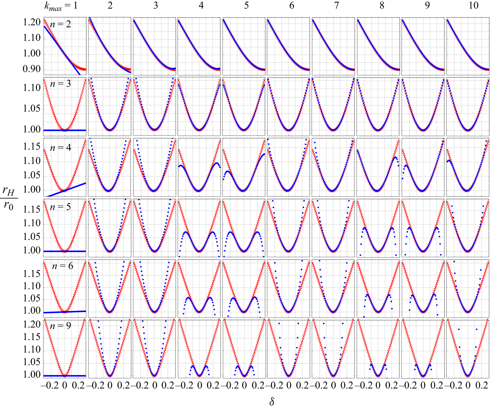
Figure 1. The ratio of hydrodynamic radius to the radius of the unit reference sphere,  $r_0 = 1$, based on asymptotic (blue dots) and direct (red crosses) methods for different geometries, parameterized by the pair $(n, \delta )$. The rows correspond to different shape functions parametrized by $n$, and the columns represent the cutoff value $k_{max}$ in (2.12).
To determine the range of validity of  $\delta$ for each $n$ and $k_{max}$, we define $\delta _{1\,\%}$ as the maximum value of the deformation amplitude at which the difference between the asymptotic and direct methods is $1\,\%$ of the direct method value. Figures 2(a) and 2(b) show the value of $\delta _{1\,\%}$ for different geometry parameters $n$ and perturbation cutoff $k_\textrm {max}$ for positive and negative values of $\delta$, respectively. The value of $|\delta _{1\,\%}|$ monotonically increases up to $k_{max} = 3$, after which, for small values of $n = 2, 3$ and $4$, we observe fluctuations. With an increase in $n$, the value of $|\delta _{1\,\%}|$ almost plateaus afterward, and for $n = 7, 8$ and $9$, the first two terms, $k_{max} = 2$, provide a physically reasonable value for the hydrodynamic radius within the range $|\delta | \leqslant |\delta _{1\,\%}|$. Our observation indicates that, with an increase in $n$, both the value of $|\delta _{1\,\%}|$ and the number of terms $k_{max}$ required for the calculation of the hydrodynamic radius (2.12) in the asymptotic expansion decrease.
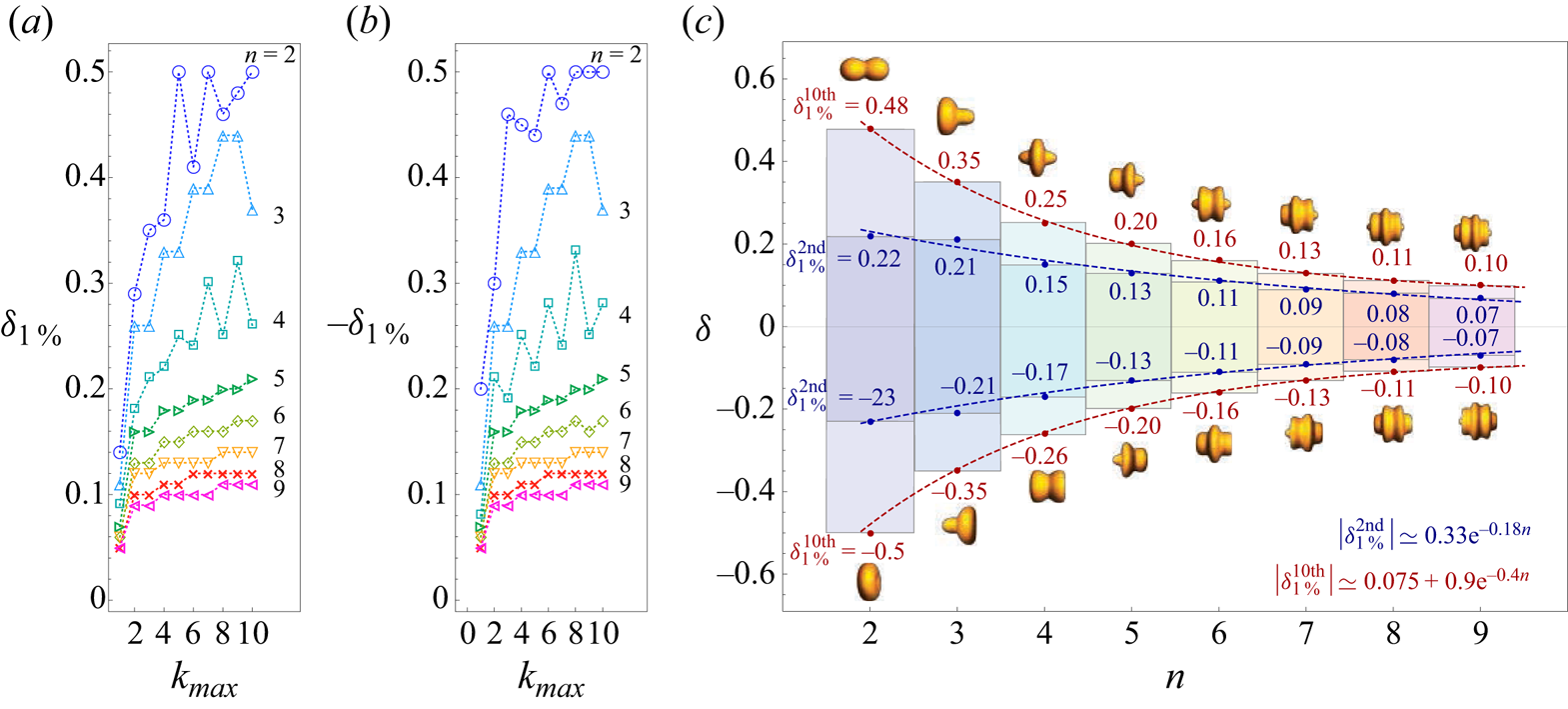
Figure 2. The maximum absolute deformation amplitude  $|\delta _{1\,\%}|$ vs perturbation cutoff $k_{max}$ for different geometric parameters $n$ for (a) positive and (b) negative values of $\delta$. (c) The range of $\delta$ as a function of the geometric parameter $n$ for the asymptotic expansion cutoff $k_{max} = 2$ and $k_{max} = 10$ with corresponding maximum deformation amplitudes $\delta _{1\,\%}^{\textrm {2nd}}$ and $\delta _{1\,\%}^{\textrm {10th}}$ for positive and negative values of $\delta$. The depicted geometries showcase the maximum deformation of unit sphere $r_0 =1$, identified by $\delta _{1\,\%}^{\textrm {10th}}$, that can be accommodated within Brenner's first mapping combined with the spectral method according to $r_{S}(\theta ) = 1 + \delta _{1\,\%}^{\textrm {10th}} \cos n\theta$.
Figure 2(c) shows the range of  $|\delta | \in [0, |\delta _{1\,\%}|]$ for the asymptotic expansion cutoff values $k_{max}=2$ and $k_{max}=10$ for the geometries studied. The geometries depicted in the figure correspond to the maximum deformation amplitude $\delta _{1\,\%}^{\textrm {10th}}$ that can be addressed within the asymptotic method for $k_{max}=10$. The geometries differ significantly from a sphere, especially for small values of $n$. Within the domain of our study, the upper limits of $\delta$ for $k_{max}=2$ and $k_{max}=10$ fit reasonably well to an exponential functions $\delta ^\textrm {2nd}_{1\,\%} = 0.33 \textrm {e}^{- 0.18 n}$ and $\delta ^\textrm {10th}_{1\,\%} = 0.075 + 0.9 \textrm {e}^{- 0.4 n}$, respectively, as represented by the dashed lines in figure 2(c).
5. Conclusion
In his seminal work (Brenner Reference Brenner1964a), Brenner developed a method to study the Stokes resistance of a slightly deformed sphere by using an asymptotic expansion of the flow field in terms of the deformation amplitude. His method involved two steps: first, mapping the surface velocity field over the radially deformed sphere to the surface of a reference sphere of arbitrary radius for each order of perturbation. In the second step, he used Lamb's general solution to map the velocity field over the reference sphere to any point in the fluid. Brenner's study focused on slightly deformed spheres to the linear order in the deformation amplitude. While his mapping machinery, in principle, could handle up to any order of perturbation, going beyond the first order makes the calculations tedious and cumbersome.
Building upon Brenner's first mapping, we utilized the spectral method for axisymmetric Stokes flow (Nabil et al. Reference Nabil, Nabavizadeh, Lammert and Nourhani2022) to reformulate his mapping within a matrix-based framework that can easily handle perturbations up to any order. We demonstrated the utility of this spectral perturbative method for highly aspherical geometries by studying the Stokes resistance of deformed spheres using the hydrodynamic radius. A family of geometries parameterized by the amplitude of the deformation  $\delta$ and $n$ in $\cos n\theta$ as the deformation function was explored. We observed that the domain of $\delta$ within which we obtain accurate results for the hydrodynamic radius depends on the deformation function. Within the acceptable range of $\delta$, the first five perturbation terms provide a reasonable estimate for the hydrodynamic radius and for a high value of $n$, up to order two is sufficient.
Axisymmetric geometries form the foundation for analysing the rectilinear translational motion of microswimmers (Brady Reference Brady2011; Yariv Reference Yariv2011; Sabass & Seifert Reference Sabass and Seifert2012; Nourhani, Crespi & Lammert Reference Nourhani, Crespi and Lammert2015). The efficacy of the axisymmetric spectral method in elucidating the dynamics of microswimmers has already been showcased using the direct non-asymptotic method (Nabil et al. Reference Nabil, Nabavizadeh, Lammert and Nourhani2022). This paper's perturbative approach can be similarly employed. It allows for pinpointing which perturbation orders have a substantial impact on the observed physical phenomena. This approach offers significant insights into how deviations from sphericity (Shklyaev, Brady & Córdova-Figueroa Reference Shklyaev, Brady and Córdova-Figueroa2014; Lammert, Crespi & Nourhani Reference Lammert, Crespi and Nourhani2016; Nourhani & Lammert Reference Nourhani and Lammert2016) affect the microswimmer dynamics, furthering our understanding of the optimum geometrical configurations for microswimmers, ranging from slightly (Daddi-Moussa-Ider et al. Reference Daddi-Moussa-Ider, Nasouri, Vilfan and Golestanian2021) to highly deformed structures. The focus of this paper was on determining the domain of validity of Brenner's first mapping, which addresses axisymmetric solid particles, a topic frequently studied in the field of microswimmers. The natural next step is to extend this formalism to non-axisymmetric, three-dimensional solid particles, and to incorporate additional spectral modes to address deformations in drops and similar mappings (Vlahovska, Loewenberg & Blawzdziewicz Reference Vlahovska, Loewenberg and Blawzdziewicz2005; Vlahovska, Bławzdziewicz & Loewenberg Reference Vlahovska, Bławzdziewicz and Loewenberg2009).
Acknowledgements
We extend our sincere gratitude to P.E. Lammert for his insightful discussions and valuable comments.
Funding
The work is supported by the National Science Foundation CAREER award, grant number CBET-2238915.
Declaration of interests
The author reports no conflict of interest.


 Open access