


1. Introduction
Aquatic vegetation, or macrophytes, modulate the spatial and temporal hydrodynamics within riverine and coastal environments. Vegetation regulates turbulence and mixing processes, which, in turn, control ecological and morphological system functions (Waycott et al. Reference Waycott2009; Nepf Reference Nepf2012). Associated flow alterations can reduce sediment transport and erosion rates, support nature-based protection of riverbeds and coastlines (Luhar, Rominger & Nepf Reference Luhar, Rominger and Nepf2008; Christianen et al. Reference Christianen, van Belzen, Herman, van Katwijk, Lamers, van Leent and Bouma2013; Luhar & Nepf Reference Luhar and Nepf2013) and influence the broad-scale morphodynamics (Cotton et al. Reference Cotton, Wharton, Bass, Heppell and Wotton2006; Vacchi et al. Reference Vacchi, De Falco, Simeone, Montefalcone, Morri, Ferrari and Bianchi2017). Turbulent fluxes and particulate exchange between canopies and free-stream flow are intrinsic to nutrient mixing, providing favourable conditions that support biodiversity (Edgar Reference Edgar1990; Clarke Reference Clarke2002) along with altering carbon capture (Prentice et al. Reference Prentice, Hessing-Lewis, Sanders-Smith and Salomon2019). The various benefits of submerged vegetation as natural ecosystems have motivated the characterisation and quantification of canopy-induced turbulence dynamics across scales.
The in-canopy flow, canopy shear layer and coherent vortices and the penetration of turbulence into the canopy all contribute to the vertical mass transfer of dissolved species (nutrients) (Lowe et al. Reference Lowe, Koseff, Monismith and Falter2005; Falter et al. Reference Falter, Atkinson, Lowe, Monismith and Koseff2007). These processes are modulated by canopy morphology and density, which are increasingly complex in flexible canopies due to the blade motions (Weitzman et al. Reference Weitzman, Aveni-Deforge, Koseff and Thomas2013). Weitzman et al. (Reference Weitzman, Zeller, Thomas and Koseff2015) noted that the presence of biomass in the lower canopy region promotes the velocity attenuation within a canopy but does not influence the upper canopy blade deflection driven by the canopy top shear. Thus, the extent of vortex penetration is considered the dominant factor controlling in-canopy flow and the associated mass transfer.
Physical modelling has provided a unique understanding of vegetation and flow interactions. In particular, rigid structures forming organised and irregular arrays have been widely used to study vegetation canopies, and have provided simplified, yet highly insightful, information to quantify fundamental flow characteristics (Ghisalberti & Nepf Reference Ghisalberti and Nepf2002; Liu et al. Reference Liu, Diplas, Fairbanks and Hodges2008; Chen, Jiang & Nepf Reference Chen, Jiang and Nepf2013; Hamed et al. Reference Hamed, Sadowski, Nepf and Chamorro2017; Chung et al. Reference Chung, Mandel, Zarama and Koseff2021). Vegetation increases drag, resulting in the formation of a shear layer at the canopy top and distinct turbulence (Gambi, Nowell & Jumars Reference Gambi, Nowell and Jumars1990; Nepf & Vivoni Reference Nepf and Vivoni2000). In flexible canopies, the vegetation deflection modulates the spatial and temporal dynamics, whereby canopy streamlining and drag reduction occur under sufficient hydrodynamic forcing (Ghisalberti & Nepf Reference Ghisalberti and Nepf2009; Luhar & Nepf Reference Luhar and Nepf2011). Ikeda & Kanazawa (Reference Ikeda and Kanazawa1996) observed intermittent, elliptical-shaped vortices forming at the canopy top that resulted in the so-called monami, evidenced by depression during the transit and waving motion of aquatic vegetation (see basic illustration in figure 1). Ghisalberti & Nepf (Reference Ghisalberti and Nepf2002) defined this region as a mixing layer, whereby streamwise velocity fluctuations correspond to the Kelvin–Helmholtz (KH) frequency. As such, monami is driven by comparatively strong sweep events ( $u' > 0$, $w' < 0$; where $u'$ and $w'$ denote the streamwise and vertical velocity fluctuations) at the vortex front, followed by a weak ejection ( $u' < 0$, $w' > 0$) at the vortex rear, due to the downward and upward side of translational hairpin vortex evolution over the canopy (Ghisalberti & Nepf Reference Ghisalberti and Nepf2002, Reference Ghisalberti and Nepf2006; Finnigan, Shaw & Patton Reference Finnigan, Shaw and Patton2009; Okamoto & Nezu Reference Okamoto and Nezu2009). The influence of canopy motion and turbulence has also been investigated in wave- and wave–current-driven flows (Zeller et al. Reference Zeller, Zarama, Weitzman and Koseff2014; Zhang, Tang & Nepf Reference Zhang, Tang and Nepf2018). However, the dynamics is not directly comparable, and the focus is placed on unidirectional flows herein.

Figure 1. Basic features common in aquatic vegetation canopies. Here,  $t_{ml}$ represents the mixing layer and $\Delta U$ indicates the associated bulk velocity difference. Stem wake flow may not occur in fully flexible stems as discussed below.
Recent numerical modelling of flexible and semi-rigid canopies by Marjoribanks et al. (Reference Marjoribanks, Hardy, Lane and Parsons2017) revealed features of turbulent fluctuations corresponding to KH vortices within the mixing layer of the canopy, along with additional distinct turbulence scales associated with canopy motion. The unsteady blade dynamics of a flexible canopy remains partially understood, particularly with respect to the spatial quantification of turbulence and exchange within and above the canopy. The spatial dynamics of coherent vortices within the canopy mixing layer under a unidirectional flow has mostly been inferred using visualisation techniques with, for example, dye (Ghisalberti & Nepf Reference Ghisalberti and Nepf2005) and long exposure imaging (Christianen et al. Reference Christianen, van Belzen, Herman, van Katwijk, Lamers, van Leent and Bouma2013).
Comparatively few studies have conducted quantitative measurements of the spatio-temporal features of turbulence associated with aquatic vegetation canopies. Instantaneous flow measurements by Nezu & Sanjou (Reference Nezu and Sanjou2008) using particle image velocimetry (PIV) showed the characteristics of coherent vortices for a flexible canopy, where coherent flow structures exhibited a greater degree of organisation near the vegetation edges than within the canopy. Okamoto & Nezu (Reference Okamoto and Nezu2009) explored the interaction between flow and blade motion using a phase-averaged approach, revealing that maximum vertical momentum transport occurs when vegetation is at the maximum and minimum of the deflected heights. Sweep events appeared to penetrate the canopy, whereas ejections mostly remained above the canopy top. Okamoto, Nezu & Sanjou (Reference Okamoto, Nezu and Sanjou2016) evaluated various canopy heights and noted that vortical structures are less coherent above a flexible canopy than over a rigid canopy, and do not penetrate into the lower parts of the canopy, the stem wake region. However, alteration to blade flexural rigidity associated with varying blade lengths was not accounted for, which has been found to influence canopy turbulence (Zhang et al. Reference Zhang, Tang and Nepf2018). Cross-spectral analysis between flow velocity and blade deflection by Okamoto et al. (Reference Okamoto, Nezu and Sanjou2016) showed that several rows could be deflected in phase with one another and in near unison, and the number of waving elements was dependent on the length scale of turbulence structures. Chen et al. (Reference Chen, Jiang and Nepf2013) also used PIV to evaluate time-averaged turbulence from the leading edge of a rigid canopy but did not acquire measurements for a flexible canopy, and optical constraints did not allow assessment of the flow structures within the canopy. A large fraction of the research regarding spatio-temporal processes has focused on the dynamics of the flow above canopies, especially in seagrass canopies. In contrast, understanding flow interactions within the canopy are not well developed, despite their known importance to, for example, bed sediment transport processes. The research presented herein overcomes challenges of obtaining optical clearance within the canopy by employing refractive-index-matching (RIM) techniques using a dynamically equivalent flexible canopy.
Various studies have quantified coherent vortices and isolated blade motions, and distinct differences in motion and turbulence dynamics have been linked to canopy morphology. Singular flexible vegetation elements deflect to a greater extent than when located within a canopy (O'Connor & Revell Reference O'Connor and Revell2019), thus altering the vertical distribution of stresses and canopy motion. Wilson et al. (Reference Wilson, Stoesser, Bates and Pinzen2003) found that the presence of plant fronds, as opposed to a single rod, resulted in increased momentum absorption and turbulent mixing. Furthermore, vegetation foliage may promote a quasi-periodic velocity within the mixing layer due to the increased vortex coherence (Caroppi et al. Reference Caroppi, Västilä, Järvelä, Rowiński and Giugni2019). O'Connor & Revell (Reference O'Connor and Revell2019) showed that monami behaviour is a function of the natural blade frequency and the mixing layer instability frequency, resulting in the spatial and temporal canopy dynamics being associated with combined fluid–structure interaction. The spatial configuration of the vegetation element within a canopy is also an important factor; Liu et al. (Reference Liu, Diplas, Fairbanks and Hodges2008) noted a substantial reduction in streamwise in-canopy velocity when stems were staggered as compared with a linear arrangement. Importantly, these studies emphasise the importance of studying canopies that are comparable to natural environments. Geometrically and dynamically scaled models may enable representative canopy motion dynamics to be replicated and thus allow for the quantification of the hydrodynamics within aquatic canopies.
The dynamics of coherent flow structures and their spatio-temporal evolution above and within canopies remains poorly understood, particularly with respect to the interaction of coherent vortices associated with KH instability within canopies. This investigation focuses on the spatial and temporal dynamics of a canopy representative of the common seagrass species Zostera marina. The analysis is complemented by a comparative assessment of flows over and through a rigid canopy to provide a broader view of a diverse range of biota-flow environments, including coral reefs, salt marshes and mangroves. The use of a large-scale RIM methodology provides unobstructed optical access to flow structures throughout the canopies from bed to free stream, permitting the acquisition of high resolution spatial and temporal flow field measurements within a comprehensively scaled vegetation canopy. The set-up of the experimental facility and design of scaled vegetation is described in § 2. Statistics and spatio-temporal analysis of the turbulence are discussed in § 3, and the principal conclusions are given in § 4.
2. Experimental set-up
Turbulence within, and above, a surrogate aquatic seagrass and a rigid canopy was studied under various flow conditions (§ 2.2) in the large recirculating RIM flume at the University of Illinois. The facility has a test section of 2.50 m length, 0.45 m width and 0.5 m height, operated in free surface mode. The RIM was achieved by matching the refractive index of the polypropylene elements with the working fluid solution, thus rendering the vegetation nearly invisible when submerged and exposed to a 532 nm wavelength light. The working fluid consists of an aqueous sodium iodide (NaI) solution at approximately 63 % by weight, with density  $\rho _{f} \approx 1780\ {\rm kg}\ {\rm m}^{-3}$ and kinematic viscosity $\nu \approx 1.1 \times 10^{-6}\ {\rm m}^{2}\ {\rm s}^{-1}$; its temperature is kept constant to ensure optimum optical access. Additional information on the RIM technique and facility are given in Blois et al. (Reference Blois, Christensen, Best, Elliott, Austin, Dutton, Bragg, Garcia and Fouke2012, Reference Blois, Bristow, Kim, Best and Christensen2020) and Bai & Katz (Reference Bai and Katz2014).
2.1. Surrogate seagrass canopy
The flexible canopy design considered dynamic scaling representative of plant structures, as well as dimensions and mechanical properties of a common coastal seagrass species Zostera marina (de los Santos et al. Reference de los Santos, Onoda, Vergara, Pérez-Lloréns, Bouma, La Nafie, Cambridge and Brun2016). Structural and morphological comparability also exists with freshwater eelgrass, specifically those under the genus Vallisneria.
Each flexible element of the canopy consisted of four rectangular blades, simulating vegetation leaves, attached to a rigid 20 mm long, cylindrical stem of diameter 6.35 mm; see figure 2. Dynamic scaling was achieved through assessment of two dimensionless parameters, namely, the Cauchy number,  $Ca$, representing the ratio of drag to rigidity force, and the Buoyancy parameter, $B$, representing the ratio of buoyancy to rigidity forces (Luhar & Nepf Reference Luhar and Nepf2016)
 \begin{equation} Ca=\frac{{\rho }_{f}b U^{2}_0{ l}^{3}}{EI} \quad\text{and}\quad B=\frac{\left({\rho }_f- {\rho }_v\right){gbdl}^{3}}{EI} \end{equation}
where  ${\rho }_v$ is the blade density, $b$ and $d$ are the blade width and thickness, $l$ is blade length, $U_0$ is incoming bulk velocity defined by the cross-sectional area of the fluid and the incoming flow discharge, g is the acceleration due to gravity, $E$ is Young's modulus and $I$
$I$  $({=}{bd^{{3}}}/{{12}})$ is the second moment of inertia.

Figure 2. (a) Basic schematic illustrating surrogate, undeflected seagrass in the RIM test section, and the field of view; (b) details of a surrogate four-blade seagrass unit, and (c) top view of the staggered arrangement of the seagrass units; here, the dashed green line indicates the location of the PIV wall-normal plane.
Particular emphasis was placed on matching  $B$ due to the naturally large variability in $Ca$ associated with the differing flow velocities considered herein. To achieve appropriate scaling, the blades were made from a polypropylene polymer of ${\rho }_v = 870 \pm 25\ {\rm kg}\ {\rm m}^{-3}$, $b = 4.13 \pm 0.18\ {\rm mm}$, $d = 0.112 \pm 0.005\ {\rm mm}$, $l = 100\ {\rm mm}$ and $E = 1.32 \pm 0.12\ {\rm GPa}$, resulting in $B = 6.59 \pm 0.80$. All error values indicate one standard deviation from the sample set mean ( $n = 20$). The blades are comparable to the model Zostera marina blades implemented by Ghisalberti & Nepf (Reference Ghisalberti and Nepf2002) and representation of Posidonia australis seagrass by Abdolahpour et al. (Reference Abdolahpour, Ghisalberti, McMahon and Lavery2018), with $B$ values ranging from 6.43 to 7.06.
The resulting flexible canopy (henceforth referred to as surrogate seagrass or simply seagrass) had an undeflected height of  $h_c= 120$ mm. Given that the blade geometry alters the reconfiguration behaviour (Albayrak et al. Reference Albayrak, Nikora, Miler and O'Hare2012), care was taken to ensure the consistent arrangement of blades around each stem (figure 2b). Vegetation elements were mounted in a staggered arrangement (figure 2c) at a density of $569\ {\rm stems}\ {\rm m}^{-2}$ along a 1.435 m ( $\Delta x/h_c \approx 12$) canopy length spanning the flume width. A roughly comparable rigid vegetation canopy was made with uniform acrylic rods of diameter $d_r= 6.35$, a height of $h_c=120$ mm from the baseboard and vertically mounted in the same staggered configuration as the surrogate seagrass (figure 2c). This rigid canopy served as a complementary base case that helped to identify the role of motion associated with flexible canopies, along with providing an elementary analogue to mangrove pneumatophores and hard corals.
2.2. Experimental conditions
Two sets of five experiments were conducted for the surrogate seagrass and rigid canopy (table 1), where,  $h_d=(h_{d,max}+h_{d,min})/2$ denotes the mean deflected canopy height, and $A_w = {(h_{d,max}-h_{d,min})}/{2}$ represents the vertical amplitude of the canopy oscillations in which $h_{d,max}$ and $h_{d,min}$ denote the average maximum and average minimum heights.
Table 1. Summary of the experimental cases and basic parameters.  $U_{\infty }$ and $U_0$: free-stream and bulk velocities; $Re$,
$Re$,  $Fr$ and $Ca$: Reynolds, Froude and Cauchy numbers; $h_{d}$: mean canopy height, $A_{w}$: vertical amplitude of the canopy motions and NA: not applicable.

The surrogate seagrass and rigid canopy were investigated at Reynolds numbers,  $Re = {U_0H_0}/{\nu } \in [3.5\times 10^{4}, 1.1\times 10^{5}]$, ( $Re_{R_h} = {U_0 R_h}/{\nu } \in [1.3\times 10^{4}, 4.0\times 10^{4}]$ based on the hydraulic radius, $R_h$), where $U_0$ is the incoming bulk velocity, and $H_0/h_c\approx 3.1$ ( $H_0=0.373$ m) is the water depth at the flume entrance, and under subcritical conditions with Froude numbers of $Fr=U_0/\sqrt {gH_0}\leqslant 0.26$, where $U_{\infty }$ is the free-stream velocity, and $g$ is gravitational acceleration. Instantaneous flow fields were acquired at $x/h_c\geqslant 9.5$, with $x=0$ denoting the beginning of the canopy. Bailey & Stoll (Reference Bailey and Stoll2016) noted that larger spanwise-oriented structures within a mixing layer maintain coherence. Image pairs were obtained using a high-speed, 4 MP ( $2560\ {\rm pixels} \times 1600\ {\rm pixels}$) CMOS camera with a 60 mm lens at a frequency of 100 Hz. The field of view (FOV) of the flexible canopy spanned $\Delta x/h_c= 2.2$ horizontally and extended $\Delta z/h_c = 1.6$ vertically from the bed. A complementary FOV covering $\Delta x/h_c= 1.4$ and $\Delta z/h_c= 2.2$ from the bed was also included, which provided a total of 2850 and 4940 image pairs for the rigid and flexible cases, respectively. The FOVs were illuminated with a 1 mm thick light sheet provided by a $250\ {\rm mJ}\ {\rm pulse}^{-1}$ double-pulsed laser supplied by TSI. The flow was seeded with $13\,\mathrm {\mu }{\rm m}$ hollow glass silver-coated particles with a density of $1800\ {\rm kg}\ {\rm m}^{-3}$. Data processing of image pairs was conducted using TSI Insight 4G software with an interrogation window of $24 \ {\rm pixels} \times 24\ {\rm pixels}$ with 50 % overlap, providing a vector grid spacing of $\Delta x = 1.64$ mm and $\Delta z= 1.22$ mm.
2.3. Basic features of the motions – visualisation
The ten cases investigated covered various flow and blade motions with different degrees of interaction between flow above and within the canopy and seagrass oscillations. The blades underwent swaying for the lowest flow ( $Re=3.5\times 10^{4}$, $Ca = 120$), and progressed into coherent waving motion representative of monami by $Re=5.3\times 10^{4}$, $Ca = 279$, which modulated the unsteady momentum exchange between the inner and outer canopy flows.
Supplementary movies available at https://doi.org/10.1017/jfm.2021.1142 illustrating the streamwise velocity fluctuations in the full FOV field within and above the seagrass (supplementary movie 1) and rigid canopy (supplementary movie 2) for the  $Re=1.1\times 10^{5}$ (F5 and R5 scenarios; table 1) aid appreciation of the rich multiscale dynamics, and reveal the signature of coherent structures. Hereon, we analyse these flows and blade interactions and characterise the dominant motions and their role in seagrass dynamics and unsteady flow exchange.
3. Results
Here, we first quantify and discuss the flow statistics within and above the surrogate seagrass; then, we inspect spatial and temporal features of the dominant coherent motions. Comparison with a rigid canopy is also included to aid insight into specific processes induced by the surrogate seagrass.
3.1. Temporally and spatially averaged turbulence statistics
The canopy boundary layer and inner flow within the surrogate seagrass exhibited significant departure from the rigid counterparts, which were modulated largely by the blade swaying. Basic flow statistics within and above the flexible and rigid canopies for a representative case at  $Re = 7.0 \times 10^{4}$ (i.e. F3 and R3 scenarios; table 1) evidence the impact of the surrogate seagrass on the flow. This is illustrated in figure 3 with the dimensionless streamwise velocity, $U/U_{\infty }$, kinematic shear stress, $-\langle u'w'\rangle /U_{\infty }^{2}$, and turbulence intensity of the streamwise, ${\sigma _u} /U_{\infty }$, and vertical, $\sigma _w /U_{\infty }$ components. Here, $()'$ indicates temporal fluctuations and $\sigma$ and $\langle \rangle$ denote the standard deviation and time-averaging operators.

Figure 3. Time-averaged streamwise velocity  $U/U_{\infty }$, kinematic shear stress, $-\langle {u'w'}\rangle /U_{\infty }^{2}$, and turbulence intensity of the streamwise, $I_u = {\sigma _u}/U_{\infty }$, and vertical,
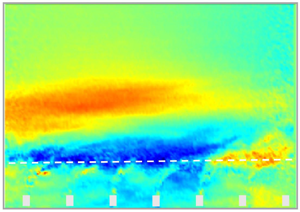
  $I_w = {\sigma _w}/U_{\infty }$, velocity components within and above the surrogate seagrass (a,c,e,g) and rigid canopy (b,d,f,h) at $Re = 7.0 \times 10^{4}$ (F3 and R3 scenarios; table 1). The horizontal, white dashed lines approximately mark the inner (within canopy) and outer flows.
The deflected blades significantly restricted the mass flux within the surrogate seagrass and enhanced the turbulence surrounding the top as compared with the rigid canopy. This resulted in a sharper mean shear that promoted unsteady exchange with the external flow, resulting in increased kinematic shear stress and turbulence levels. This, in turn, promoted oscillations of the canopy elements, which enhanced unsteady flow exchange and flow fluctuations near the top of the surrogate seagrass. The degree of such two-way interaction between the flow and blade motions is embodied in the Cauchy number. Evaluation of scenarios encompassing a range of  $Ca$ provides context for natural flows, and offers a way to uncover several processes, including the control of flow fluctuations and particulate transport.
Double averaging in the streamwise direction and time (figure 4) illustrates distinct features of the bulk flow statistics across the vertical span for a range of  ${Re}$ in the seagrass and rigid canopy. The vertical axis is split into two non-dimensional regions to aid understanding of the effect of the deflection of the flexible canopy. The canopy region is normalised by the mean deflected canopy height, i.e. $z/h_d$; whereas the region above the canopy is normalised as $z_{A}=(z-h_d)/h_c+1$. This factor sets the relative canopy top as a secondary origin. Note that the non-dimensional streamwise velocity, $U/U_{\infty }$ profiles collapse very well within and above the rigid canopy and $z_{A}$ is not normalised by the boundary layer depth, $\delta$, to stress the flow variability induced by the flexible canopy. In contrast to the seagrass, the rigid canopy did not alter development of the boundary layer at the $Re$ analysed. It is also worth highlighting the changing profiles within the seagrass canopy with changes in $Re$. This is further illustrated by the velocity change $\Delta U/U_{\infty }=(1-U_c/U_{\infty })$ within and above the canopies (figure 5a), which is approximately constant for the rigid canopy but decreases with $Re$ in the seagrass experiments.

Figure 4. Space- and time-averaged vertical profiles of the normalised (a) streamwise velocity  $\bar {U}/U_{\infty }$, and (b) kinematic shear stress $-\langle \overline {u'w'}\rangle /U_{\infty }^{2}$. Turbulence intensity of the streamwise (c) $\overline {I_u} = \overline {\sigma _u} /U_{\infty }$ and vertical (d) $\overline {I_w} = \overline {\sigma _w}/U_{\infty }$ velocity components. The overbar denotes space-averaging. Vertical axis is normalised by the deflected canopy height $h_d$, and the shaded area represents the data within the canopy.

Figure 5. (a) Velocity change within canopy, (b) mixing layer thickness, (c) vortex penetration depth relative to the undeflected canopy height (left axis) and vortex penetration relative to the deflected canopy height (right axis). Data are shown for both the flexible seagrass and rigid canopy.
A distinct effect induced by the surrogate seagrass is the relative height of the maximum kinematic shear stress (figure 4b), which does not occur within the vicinity of the mean canopy top due to the particular modulation of the blade oscillations. Note the lower kinematic shear stress compared with, e.g. Ghisalberti & Nepf (Reference Ghisalberti and Nepf2006) and Chung et al. (Reference Chung, Mandel, Zarama and Koseff2021). This is due to the shorter canopy length  $L_c$ and the relative FOV location. Indeed, the canopy length $L_c = 1.435$ m (figure 2a) is shorter than those in Ghisalberti & Nepf (Reference Ghisalberti and Nepf2006) and cases in Chen et al. (Reference Chen, Jiang and Nepf2013) and Chung et al. (Reference Chung, Mandel, Zarama and Koseff2021). As pointed out by Chung et al. (Reference Chung, Mandel, Zarama and Koseff2021), the maximum shear stress increases with $L_c$. Additionally, our FOV measured the developing region of the mixing layer. Chen et al. (Reference Chen, Jiang and Nepf2013) showed that the development length $X_* \approx (8 \pm 2) {U_vL_S}/{u_*}|_{h_c}$, where $U_v, L_S$ and $u_*$ are the vortex convection velocity, shear length scale and friction velocity at the canopy top; Chung et al. (Reference Chung, Mandel, Zarama and Koseff2021) showed that the shear length scale can be estimated as $L_{s}=\bar {U}/{\partial \bar {U}}/{\partial z}|_{h_c}$, resulting in $L_s \approx 0.04$ m and $X_* \approx 1.75 \pm 0.44$ m for the R1 case. This indicates that our FOV is in the developing region of ${\approx }0.72X_*$, which also leads to lower kinematic shear stress, as shown in Chen et al. (Reference Chen, Jiang and Nepf2013) and Chung et al. (Reference Chung, Mandel, Zarama and Koseff2021). It is worth stressing the importance of this region given the heterogeneity or patchiness of natural canopies affected by various topographic factors and morphological features, including width, shape factor, rigidity and orientation of the blades. Remarkably, the associated streamwise component, expressed here as turbulence intensity $\bar {I}_u$, occurred below the mean canopy height. The particular locations of the maximum in $-\langle {u'w'}\rangle$ at $z/h_d>1$ and $\langle {u'u'}\rangle$ at $z/h_d<1$ in the seagrass indicate a transport modulated by the motion of the blades, which is very different from the rigid counterpart and represent a signature of the distinct scale-to-scale dynamics. The higher turbulence momentum flux above the seagrass canopy, indicated by larger magnitude $-\langle \overline {u'w'}\rangle$, suggests greater mass transfer within the canopy. The deflection of flexible blades during the passage of coherent vortices reduces the exposed blade surface area, and thus the potential uptake of e.g. dissolved inorganic nitrogen relative to separated blades during weaker flows (Weitzman et al. Reference Weitzman, Aveni-Deforge, Koseff and Thomas2013). Furthermore, the extent of the $-\langle \overline {u'w'}\rangle$ within the canopies (figure 4b) provides an indication of the vortex penetration depth, ${\delta }_e$, given by the distance below $h_d$ whereby kinematic stress decreases to 10 % of the maximum (Nepf & Vivoni Reference Nepf and Vivoni2000). Evaluation of vortex penetration depth normalised by deflected canopy height ( $h_d$) indicates vortex penetration towards the bed was smaller for the flexible canopy than the rigid canopy at lower $Re$, but increased with larger $Re$ (figure 5c).
The mixing layer thickness,  $t_{ml} = z_2-z_1$, where $z_1$ and $z_2$ denotes the height of the 99 % free-stream and in-canopy velocities, remained nearly constant for the rigid canopy with $Re$ (figure 5b), with an asymmetrical vertical distribution with approximately one third below $h_c$, similar to the observations of Ghisalberti & Nepf (Reference Ghisalberti and Nepf2004). Ghisalberti & Nepf (Reference Ghisalberti and Nepf2002) found monami occurred when $t_{ml}/h_d > 1.5 - 2.1$, which is the case here, whereby $t_{ml}/h_d$ ranges between 1.4 and 2.0, with the lowest $Re$ condition not initiating coherent waving representative of monami. Ghisalberti & Nepf (Reference Ghisalberti and Nepf2002) also noted that waving increases the vortex penetration depth (normalised by $h_d$) and suggested that waving canopies induce a weaker momentum sink compared with rigid cases. However, Nepf & Ghisalberti (Reference Nepf and Ghisalberti2008) reported no difference in dimensional $\delta _{e}$ vs waving and un-waving canopies. Alternatively, when evaluated in dimensional terms based on the fixed dimension of $h_c$, the flexible canopy vortex penetration depth does not increase with $Re$ and remains smaller than the rigid canopy, revealing that the flexible canopy limits the depth of stresses (see figure 5c). It is worth pointing out that Okamoto & Nezu (Reference Okamoto and Nezu2009) inspected penetration of coherent structures within a flexible canopy composed of an array of single elements and suggested that, regardless of differences in vegetation morphology, the role of canopy reconfiguration associated with flexibility plays a dominant role in reducing the vertical penetration of stresses. However, Wilson et al. (Reference Wilson, Stoesser, Bates and Pinzen2003) noted the role of foliage morphology, where a smaller penetration of turbulent stresses occurred for rods with fronds (similar to flexible blades) than rods alone, and suggested that the presence of the fronds limited the momentum exchange between the canopy and overlying flow.
The redistribution of the Reynolds stresses induced by the seagrass can be further assessed by inspecting the velocity fluctuations into four quadrants, namely  $Q_1$: $u' >0$, $w'>0$ (outward interactions), $Q_2$: $u'<0$, $w'>0$ (ejections), $Q_3$: $u'<0$, $w'<0$ (inwards interactions) and $Q_4$: $u'>0$, $w'<0$ (sweeps). Specifically, figure 6 illustrates the spatial distribution of the sweep-to-ejection ratio, $Q_4/Q_2$, for selected cases. Consistent with Yue et al. (Reference Yue, Meneveau, Parlange, Zhu, van Hout and Katz2007), Poggi et al. (Reference Poggi, Porporato, Ridolfi, Albertson and Katul2004) and Chen et al. (Reference Chen, Jiang and Nepf2013), the base cases with the rigid canopy exhibited a predominance of sweeps within the canopy for all $Re$ tested. However, ejections dominated within the surrogate seagrass with comparatively strong sweeps in the vicinity of the mean canopy height. Note also the distinct modulation of the blade motions in the distribution of $Q4/Q2$ in the boundary layer. Although sweep-dominated events appear on the rigid canopy at the $Re$ studied, those were only present in the lower half of the flexible canopy ( $z/h_d < 0.5$) at the lowest ${Re}$ (figure 6a); the minimal blade deformation at that $Re$ made it comparable to that in the rigid canopy. Figure 6 also shows a phenomenon not previously reported, namely, the transition to ejection-dominated events with $Re$ within the seagrass. The upward motion of the blades associated with the ejection at the rear of vortices may result in ejection events. Likewise, the deflection of blades prevents penetration of sweep events as per the rigid canopy. This is also consistent with the arguments by Okamoto et al. (Reference Okamoto, Nezu and Sanjou2016), who pointed out that coherent structures do not extend into the lower canopy region under monami.

Figure 6. Ratio of total contribution of sweep ( $Q4$) and ejection ( $Q2$) events for the seagrass scenarios (a) F1, (b) F3, (c) F5 and rigid canopy cases (d) R1, (e) R3, (f) R5. Dashed white lines indicate the mean canopy height.
The region with the largest sweep-dominated motions was consistently located at the vicinity of the mean deformed seagrass height,  $h_d$, in agreement with other findings (Nezu & Sanjou Reference Nezu and Sanjou2008; Marjoribanks et al. Reference Marjoribanks, Hardy, Lane and Parsons2017). The differences in the magnitude of the sweep-to-ejection ratio between the surrogate seagrass and rigid canopy are likely due to the ability of the blade motion to promote turbulent transport. Bailey & Stoll (Reference Bailey and Stoll2016) suggested that a canopy impedes a vortex to draw fluid from below, thus limiting the presence of ejections near the canopy top. In contrast, sweeps dominate due to their ability to draw flow fluctuations from the unobstructed and higher momentum flow above. The deflection of blades also increases the canopy top blockage area, producing an apparent increase of the canopy density, which likely increases sweep dominance (Poggi et al. Reference Poggi, Porporato, Ridolfi, Albertson and Katul2004). In contrast, the upright blades of the rigid canopy do not provide the same top-down area blockage and constraint. Importantly, this suggests that the streamlining of the flexible canopy blades under sufficient flow results in an effective barrier to larger-scale turbulence.
3.2. On the coherent motions and flow–canopy interaction
First, we explore the combined redistribution, enhancement and damping of turbulence across relevant scales modulated by the blade motions within and above the canopy with the one-dimensional compensated spectra of the streamwise velocity fluctuations,  $f \phi (f)$, where $f$ is the frequency. Figure 7 shows this quantity normalised by the maximum value, $f{\phi }^{*}={f\phi }/\max \{f\phi \}$, throughout the vertical span at nearly the centre of the FOV ( $x/h_c = 10.25$). A low-pass filter with a 10 Hz cutoff frequency is applied to the signal; over that frequency, the energy contribution is minor. The spectral velocity distributions within the rigid canopy at three $Re$ show a comparatively dominant energy at a frequency $f_0=f_0(Re)$, corresponding to vortex shedding from the rigid structures, where the Strouhal number is $St=f_0d_r/U_1\approx 0.19 - 0.20$ (Norberg Reference Norberg1994). Such motions are missing within the seagrass; there, the turbulent energy plays a minor role compared with the above-canopy turbulence and that within the rigid canopy.

Figure 7. Compensated one-dimensional spectra of the streamwise velocity fluctuations along the vertical span at the centre of the FOV  $x/h_c = 10.25$ for (a) F1, (b) F3 and (c) F5 seagrass scenarios, and (d) R1, (e) R3 and (f) R5 rigid canopy cases. Dashed lines indicate the canopy top ( $h_d$), and dotted lines denote the location of $z_1$ and $z_2$.
Generation of KH instability (Ghisalberti & Nepf Reference Ghisalberti and Nepf2002; Okamoto & Nezu Reference Okamoto and Nezu2009; Okamoto et al. Reference Okamoto, Nezu and Sanjou2016; Marjoribanks et al. Reference Marjoribanks, Hardy, Lane and Parsons2017) appears to be associated with enhanced energy above the canopy. Considering Ghisalberti & Nepf (Reference Ghisalberti and Nepf2002), the KH frequency,  $f_{KH}$, can be estimated as follows:
 \begin{equation} f_{KH}= St\frac{\bar{U}}{\theta}, \quad \theta =\int^{\infty }_{-\infty}{\left[\frac{1}{4}-{\left(\frac{U-\bar{U}}{\Delta U}\right)}^{2}\right]{\rm d}z,} \end{equation}
where  $\bar {U}=(U_{\infty }+U_c)/2$ (see figure 1), $\theta$ is the momentum thickness and $\Delta U = U_{\infty } - U_c$ is the bulk shear magnitude. In scenarios of unforced mixing layers $St\approx 0.032$, and varies modestly with the velocity ratio $R=\Delta U/({2\bar {U}})$ by up to 5 % between $R = 0$ and 1 (Ho & Huerre Reference Ho and Huerre1984). The canopies, however, induce a distinct forcing such that the $St = 0.032$ for parallel, unforced flows is not quite applicable. Indeed, Mandel et al. (Reference Mandel, Gakhar, Chung, Rosenzweig and Koseff2019) obtained $St = 0.064$ for a rigid canopy. This illustrates the possible differences between predicted and measured frequencies presented in table 2. Another characteristic frequency of interest is the undampened natural blade frequency, estimated by
 \begin{equation} f_n\approx C_n\sqrt{{EI}/{l^{4}\left({\rho }_vbd+{\rho }_fC_M({\rm \pi} b^{2}/4)\right)}}, \end{equation}
with  $C_n= 0.56$ and $C_M\approx 1$ (Luhar & Nepf Reference Luhar and Nepf2016), which results in $f_n\approx 0.34$ Hz. Recent numerical simulations by O'Connor & Revell (Reference O'Connor and Revell2019) indicate that canopy motion is a coupled response between the natural structure (vegetation blade) and coherent flow motions. Both $f_{n}$ and $f_{KH}$ may coexist if they differ sufficiently; however, a lock-in phenomenon and canopy waving may occur when $f_{n}$ and $f_{KH}$ are similar. The transition of two modes to lock-in behaviour is captured in figure 8(b), where a weaker shear is seen to lead to a smaller $f_{KH}$ at $t \geqslant 8\ {\rm s}$, resulting in synchronisation.
Table 2. Characteristic parameters in the surrogate seagrass and rigid canopy. Strouhal number  $St$, velocity ratio $R$, estimated blade natural resonance frequency $f_n$, predicted KH frequency $f_{KH}$ and time-averaged peak spectral frequency at $z/h_d=1.05$, $f_{max}$. NA: not applicable.


Figure 8. Wavelet representation of the streamwise velocity within and immediately above the flexible (F5) and rigid (R5) canopies at  $Re=1.1\times 10^{5}$. (a) R5, $z/h_d=1.05$, (b) F5, $z/h_d=1.05$, (c) R5, $z/h_d=0.5$, (d) F5, $z/h_d=0.5$. White dashed lines indicate the cone of influence, and horizontal dotted lines mark $f_{KH}$.
A complementary inspection into the time–frequency domain with a Morlet wavelet analysis, reveals insightful features of the turbulent fluctuations in the canopy mixing layer and compact signatures within the period of the measurements, which can be obscured with velocity spectrum analysis. The cases for the highest  $Re$ (seagrass, F5, and rigid canopy, R5) scenarios are shown in figure 8 within the canopy at $z/h_d=0.5$ and immediately above the mean canopy height at $z/h_d=1.05$. The frequency associated with the predicted KH instability, $f_{KH}$, is indicated with horizontal dashed lines.
Note that the rigid canopy exhibits relatively energetic fluctuations at a frequency  $f\geqslant f_{KH}$ with higher persistence at $z/h_d=1.05$ (figure 8a). Remarkably, the velocity fluctuations in the surrogate seagrass exhibit two dominant, stronger signatures than those of the rigid canopy. One is a non-persistent, shear-induced $f_{KH}$, whereas the other is a persistent, blade-modulated signal at a lower frequency. These two distinct motions induced secondary motions between these frequencies for a short time (see figure 8b). Such an aperiodic phenomenon evidences additional nonlinearities induced by the large deformations of the blades (Jin et al. Reference Jin, Kim, Hong and Chamorro2018).
Spatio-temporal characteristics of the flow fluctuations within the canopies at  $z/h_d=0.5$ reveal distinct energetic processes contributing to the dynamics. Numerical simulations by Marjoribanks et al. (Reference Marjoribanks, Hardy, Lane and Parsons2017) noted that $f_{KH}$ was not persistent within the mixing layer in semi-rigid and flexible canopies. Here, in the rigid canopy, the flow exhibits dominance of the cylinder shedding frequency; it is not continuous across the timespan (see figure 8c). In contrast, flow in the seagrass shows the signature of KH motions at times during coordinated blade motions (see supplementary movie 1), which promoted the generation of KH-like motions into the canopy (see figure 8d). Under uncoordinated blade motions, there is a lack of KH-like motions. The averaged vortex penetration remains reduced by the seagrass under uncoordinated blade motions.
Inspection of selected instants offers insight into the underlying effects of the sweeps and ejections. In particular, the seagrass F5 case is considered herein, using two points for interrogation, with one above and one within the canopy at nearly the centre of the FOV, ( $x/h_c$, $z/h_d)=(10.25, 1.3)$ and (10.25, 0.4). From the resultant time series of $u'/U_{\infty }$, $w'/U_{\infty }$, and associated $-\langle u'w'\rangle /U_{\infty }$, we can observe instants with sweeps (e.g. $t= 4.25$ s, 5.91 and 7.30 s) and ejections (e.g. $t=5.28$ s and 6.46 s). The time series and selected times are indicated in figure 9(a). The red lines correspond to instants with alternating $u'$ above and within the canopy. Above the canopy, the sweep events correspond to positive $u'$ and negative $w'$, while ejection events express the opposite trends. The $u'w'$ values peaked with each event, yet the weak ejection event at $t = 5.28$ s represents a notably lower Reynolds shear stress. The behaviour within the canopy is less clear, which may suggest a lag in processes between the two regions.

Figure 9. (a) Selected snapshots of the streamwise velocity fluctuations for the F5 case; sweeps at  $t h_d/ U_{\infty } = 0$, $\approx$0.2 and $\approx$0.4 and ejections at intermediate times $t h_d/U_{\infty }\approx 0.1$, and $\approx$0.3. The blades around the top are shown with black lines. (b) Time series of streamwise, $u'/U_{\infty }$, and vertical, $w'/U_{\infty }$, velocity fluctuations and kinematic shear stress, $-\langle u' w'\rangle /U_{\infty }$, at $z/h_d = 1.3$ and $z/h_d= 0.4$ at $x/h_c = 10.25$. The vertical red lines correspond to the instants in (a).
The associated whole flow fields at the instants selected are shown in figure 9(b). The canopy experienced a depression of the blades in correspondence with the sweep events, followed by upward motion during ejection events. This waving motion of the canopy is comparable to previously reported monami processes (Ikeda & Kanazawa Reference Ikeda and Kanazawa1996; Ghisalberti & Nepf Reference Ghisalberti and Nepf2002). Details of the motions are shown in the supplementary movie 1.
Specific, quantitative insight into the key coherent structures and their dynamics can be obtained with SPOD. As a data-driven modal analysis technique, SPOD utilises empirical data and combines the merits of the traditional space-only POD and dynamic mode decomposition (DMD). SPOD extracts structures that are spatially and temporally coherent instead of the spatial-only coherence of POD. The SPOD modes are also optimal-averaged DMD modes (Tu et al. Reference Tu, Rowley, Luchtenburg, Brunton and Kutz2014), which contain the inherent energy ranking and form on an orthogonal basis for the flow field, like the POD-based techniques first proposed by Lumley (Reference Lumley1970). Herein, the SPOD approach follows Sieber, Paschereit & Oberleithner (Reference Sieber, Paschereit and Oberleithner2016).
First, the so-called Welch method is used to construct an ensemble of realisations of the temporal Fourier transform of the data from a single time series consisting of  $N_T$ snapshots by breaking it into several segments. Each of these consists of $N_{FFT}$ snapshots, and overlaps with the next segment are preferred to account for the statistical variability of the turbulent flow. Here, $N_{T} = 9000$, is the number of the zero-padding snapshot series, and $N_{FFT} = 1024$, which allowed us to achieve a resolution in the frequency domain of $\approx$1 Hz. A discrete Fourier transform is then applied on the separated time-dependent segment realisations, $q^{k}_{T_j}$, where $k$ stands for the $k{\rm th}$ realisation of the vector of observations, and $T_j$ is the instant. It allows us to obtain the coefficient $\hat {q}^{k}_{f_m}$ in the Fourier domain, where
 \begin{equation} \hat{q}^{(k)}_{f_{m}}=\sum_{j=0}^{N_{{FF}}-1} q^{(k)}\left(t_{j+1}\right) \exp({-{\rm i} 2 {\rm \pi}j m / N_{{FFT}}}), \quad k={-}N_{{FFT}} / 2+1, \ldots, N_{{FFT}} / 2. \end{equation}
Then, for each frequency  $f_{m}$, $\hat {Q}_{f_{m}}$ may be formed as follows:
 \begin{equation} \hat{Q}_{f_{m}}=\left[\begin{array}{cccc} \mid & \mid & & \mid \\ \hat{q}_{f_{m}}^{(1)} & \hat{q}_{f_{m}}^{(2)} & \cdots & \hat{q}_{f_{m}}^{(N)} \\ \mid & \mid & & \mid \end{array}\right], \quad \hat{Q} \in \mathbb{C}^{M \times N} \end{equation}
where  $M$ is the degree of freedom given by the number of spatial points in the $x$- and $z$-directions in each case, and $N$ is the number of realisations. Singular value decomposition is then performed in each $\hat {Q}$ matrix.
We use the variance norm of a two-dimensional, two-component stochastic velocity fluctuations matrix  $\underline{u'}(x,z,t) = [u' w']^{\textrm {T}}$ for the SPOD input. Modes are optimised in the mean square value of the velocity fluctuations by utilising singular value decomposition (Taira et al. Reference Taira, Brunton, Dawson, Rowley, Colonius, McKeon, Schmidt, Gordeyev, Theofilis and Ukeiley2017). Further details regarding SPOD implementation are given in Schmidt & Colonius (Reference Schmidt and Colonius2020) and SPOD applications in Towne, Schmidt & Colonius (Reference Towne, Schmidt and Colonius2018) and Schmidt et al. (Reference Schmidt, Towne, Rigas, Colonius and Brès2018).
Application of the SPOD, particularly for the rigid R5 and seagrass F5 cases, reveals particular features of the coordinated dynamics of the flow and seagrass, and the role of energetic coherent motions. Figure 10 shows the SPOD spectra above and within the canopy of the rigid case R5, and demonstrates the mode ranking characteristic of the SPOD method. The separation between the first and lower energy modes is prominent at a lower frequency ( $\lesssim$3 Hz) and suggests that the dynamics of large coherent structures can be approximated by the first few modes using a lower rank approximation. A broader band frequency of the dominant KH-type instability occurs above and within the rigid canopy. In contrast, a higher frequency peak is observed within the canopy (figure 10b) in agreement with the two-dimensional spectra in figure 7. The spatial mode shapes associated with the dominant frequencies of the streamwise SPOD modes, $\phi _{u'}$, are illustrated in figure 11, with the red–blue colour representing the spatially correlated patterns. The mode shapes above the canopy tip demonstrate structural features consistent with the shear layer KH instability (table 2); local changes of the convective velocity cause the observed broad frequency distribution. The von Kármán vortex street past the rods exhibited the well-known Strouhal relationship, $St \approx 0.2$.

Figure 10. Spectral proper orthogonal decomposition (SPOD) spectra of the rigid R5 case of the flow field (a) above and (b) within the canopy, with the darkest (black) line being the first SPOD mode and the lighter lines the subsequent SPOD modes.

Figure 11. Spatial organisation of the first SPOD modes above the rigid R5 canopy at  $f =$ (a1) 0.88 Hz and (a2) 1.07 Hz; and within the canopy at $f=$ (b1) 0.88 Hz and (b2) 3.52 Hz.
Insight from the SPOD spectra above and below the seagrass at the same  $Re$ for the F5 case, can be obtained from figure 12. Coherent motions related to the KH frequency dominate above and below the canopy, and the corresponding mode shapes are shown in figure 13. While KH vortices have previously been discussed above seagrass canopies (Ghisalberti & Nepf Reference Ghisalberti and Nepf2002), and coherent vortices have been observed (Nezu & Sanjou Reference Nezu and Sanjou2008), these results provide compelling evidence of KH-type vortices and provide spatio-temporal information. A weaker local peak at 2.25 Hz present above the canopy suggests the existence of a weaker coherent structure (figure 13a2). However, this coherent structure with lower energy content is not able to penetrate the barrier created by the blade motion and thus is not observed for the in-canopy flow. Also, a mismatch exists between the primary mode frequency of the flow above and within the canopy, with the upper flow having the strongest mode at $\approx$0.4 Hz and the lower part at $\approx$0.6 Hz.

Figure 12. SPOD spectra of the seagrass, F5 case, of the flow field (a) above and (b) within the canopy, with the darkest (black) line being the first SPOD mode and the lighter lines the subsequent SPOD modes.

Figure 13. Spatial organisation of the first SPOD modes above the canopy at  $f =$ (a1) 0.4 Hz and (a2) 2.25 Hz; and within the canopy at $f=$ (b1) 0.6 Hz and (b2) 0.68 Hz.
To uncover particular effects of the blade motion on flow interaction above and within the canopy, SPOD is performed on the full F5 case (figure 14). Close inspection shows that the most energetic modes at  $\approx$0.4 Hz captured only the coherent structures above the canopy, whereas monami effects and entrainment of the coherent structures are better captured by the second strongest mode (see also supplementary movie 3). The inset shows the projected second mode time coefficient for the natural blade frequency and the KH frequency. Figure 15 illustrates a sequence every $\Delta th_d/U_{\infty }\approx 0.05$ within one period of the 0.6 Hz projected time coefficient. It reveals the streamwise propagation features and a monami effect with entrainment into the region within the canopy, which is not observed at 0.4 Hz due to a much weaker second mode despite its stronger first mode energy. The lack of sinusoidal-like behaviour exhibited in the 0.4 Hz projected-coefficient second mode, as compared with the 0.6 Hz counterpart, indicates that blade motion is dominated by the KH frequency rather than the natural frequency, consistent with figure 9.

Figure 14. (a) Full flow field SPOD spectrum on the seagrass F5 case. The darkest to lighter lines indicate the progression from the first to the fourth SPOD modes; (b) projected SPOD mode coefficients,  $b_{i,j}(t)$ for the $i{\rm th}$ mode of $j$ frequency.

Figure 15. Sequence uniformly distributed in a period of the second SPOD mode of  $f = 0.6$ Hz for the F5 seagrass scenario.
This description motivates inspection of the instantaneous quadrant analysis data given in figure 16(a). The 0.6 Hz peak supports our previous assumption that the switch from sweep-dominated to ejection-dominated behaviour within the flexible canopy is related to monami and the blade motion. The projected-coefficient first mode at 0.6 Hz is shown in figure 16(b). Combining this with the base analysis of § 3.1 and figure 9, it is inferred that the projected-coefficient period is associated with the canopy blade motion. The conditional sampling method provides a representation of the sweep- or ejection-dominated flow within the canopy during the phase of downward and upward blade motions (figure 17). This supports our conjecture, whereby the presence of strong ejections within the flexible canopies correspond to the upward blade motions, which coincides with the rear of the KH vortex, and previously identified above-canopy ejection events shown in figure 9 and in past research (Ghisalberti & Nepf Reference Ghisalberti and Nepf2002; Okamoto & Nezu Reference Okamoto and Nezu2009). These results reveal the complexity and diversity of within canopy processes, which are driven by the canopy motion.

Figure 16. (a) SPOD spectra form the quadrant analysis of the seagrass F5 case. The darkest to lighter lines indicate the progression from the first to the fourth SPOD modes; (b) projected SPOD mode coefficients,  $b_{1,4}(t)$ for the first mode of 0.6 Hz.

Figure 17. Conditional average of sweep to ejection ratio during the F5 flexible canopy (a) downward motion phase and (b) upward motion phase.
4. Conclusions
As highlighted in § 1, this investigation aims to contribute to our limited understanding of the dynamics of the dominant coherent flow structures and their spatio-temporal evolution above and within a canopy representative of common seagrass species. Our set-up enabled close inspection, identification and evaluation of energetic vortices and their space–time variability. The large body of previous research on canopy flows aligns with our initial results and provided support for novel insights pointed out below. The novel methods enabled quantitative analysis of inner–outer canopy interactions using a combination of time–frequency (wavelet) and conditional phase-average, low-order (Fourier-based) tools. This is only possible with full optical access and high-frame-rate flow characterisation.
While previous research has identified the presence of turbulence frequencies consistent with KH vortices above seagrass canopies, our space–time analysis provides robust and compelling confirmation through visual and statistical analysis. Furthermore, through the use of instantaneous high-speed data, time–frequency analysis reveals that these coherent vortices may have a compact extent. This indicates that KH-like vortices are inconsistent or that their magnitude varies such that the Strouhal number associated with predictions is not entirely valid. The recognition of coherent vortex variability is of considerable importance when understanding seagrass system dynamics, specifically the mixing processes and turbulent fluxes if KH presence and magnitude are assumed constant. The states dominated by KH vortices express coherent waving and monami phenomenon in agreement with previous literature, although the canopy motion amplitude is reduced when coherent vortices are diminished. Furthermore, we show that the canopy underwent phases of highly coordinated deflected motions and phases of uncoordinated blade deflections, thus varying the exposed blade surface area.
The results support previous findings that canopy deflection inhibits the entrainment of canopy top sweeps into the lower canopy regions. Yet, we further uncover new dynamics within the canopy due to the canopy motion. Specifically, we present a hypothesis based on the SPOD modes on how the canopy motion modulates the interaction between above and within canopy flows and subsequently confirm through conditional averaging that the upward canopy motion results in a dominance of ejection events within the canopy. For the first time, the results reveal that the turbulence dynamics within flexible seagrass canopies transitions from sweep to ejection as  $Re$ and $Ca$ increases; this phenomenon is absent in rigid canopies.
The conceptual schematic illustrated in figure 18 embodies the common and distinct features of the flow in the seagrass and rigid canopies. The changes in turbulence process are critical to the lower canopy processes, including the potential bedload and suspended sediment dynamics. It is worth stressing that the distribution, or characteristic profiles, of the streamwise velocity component, kinematic shear stress and turbulence kinetic energy all exhibit different features in the two scenarios. The depth-restricted stresses in the seagrass reduce mixing and extend hydraulic retention, which are fundamental to biological processes, including nutrient and particulate exchange with the outer flow and providing greater bed protection (e.g. Christianen et al. Reference Christianen, van Belzen, Herman, van Katwijk, Lamers, van Leent and Bouma2013; Ondiviela et al. Reference Ondiviela, Losada, Lara, Maza, Galván, Bouma and van Belzen2014; Guannel et al. Reference Guannel, Ruggiero, Faries, Arkema, Pinsky, Gelfenbaum, Guerry and Kim2015; Paul Reference Paul2018; Paquier et al. Reference Paquier, Meulé, Anthony, Larroudé and Bernard2019). These protective processes are not evident within the rigid canopy.

Figure 18. Schematic summary of flow processes associated with (a) rigid canopy and (b) flexible canopy based on  ${Re} \sim 10^{5}$.
Supplementary movies
Supplementary movies are available at https://doi.org/10.1017/jfm.2021.1142.
Funding
This work was supported by the Department of Mechanical Science and Engineering, University of Illinois at Urbana-Champaign, as part of the start-up package of L.P.C. The experiments were performed in a facility built under National Science Foundation grant awards CBET-0923106 and CBET-1241349. This research was conducted with the financial support of R.C.H's PhD Scholarship at the University of Hull and the Energy and Environment Institute, along with a research grant provided by the British Society of Geomorphology (BSG).
Declaration of interests
The authors report no conflict of interest.


 Open access