


1. Introduction
Today, we cannot honestly say that we are capable of accurately predicting the transition location in a boundary layer subject to free-stream turbulence (FST). Not even in the simplest boundary-layer flow, namely the one developing over a flat plate under a zero-pressure gradient condition, are we successful. There are numerous empirical relations for predicting the transition location in the presence of FST, mostly only based on the turbulence intensity ( ${Tu}$) as input, but none with an accuracy better than typically 65 % for all ${Tu}$. Thus, in a sense, we have failed in delivering a simple and reliable transition prediction model for engineering predictions, which takes both ${Tu}$ and the FST characteristic length scale into account in a physically correct way.
When a two-dimensional boundary-layer flow undergoes laminar to turbulent transition under the presence of FST, the transition scenario is different from the condition with a low background disturbance level. Under the latter condition, the initial phase of velocity disturbance growth is characterized by small-amplitude exponentially growing Tollmien–Schlichting (T–S) waves described by modal stability theory (Tollmien Reference Tollmien1929; Schlichting Reference Schlichting1933). Under the former condition, the disturbance growth is instead characterized by algebraically growing unsteady streamwise velocity streaks, and is described by non-modal stability theory (Ellingsen & Palm Reference Ellingsen and Palm1975; Landahl Reference Landahl1980; Gustavsson Reference Gustavsson1991). The designation ‘bypass transition’ is still often used when referring to FST induced boundary-layer transition, although somewhat incorrectly. The term bypass transition was according to Morkovin coined by himself (cf. Morkovin Reference Morkovin and Graham1985) in Morkovin (Reference Morkovin and Wells1969) and was introduced to denote any transition process that bypassed common knowledge or existing theories, which at the time was limited to the T–S wave transition scenario described by modal theory. Bypass as a stand-alone term, without transition, is however encountered before the introduction of the term by Morkovin, then referring to artificially forced high amplitude T–S waves, which through nonlinearity advanced the known secondary instability and breakdown to turbulence and, hence, completely bypassed the linear range of the T–S wave (Klebanoff, Tidstrom & Sargent Reference Klebanoff, Tidstrom and Sargent1962). Going back to the meaning of bypass transition by Morkovin, it was originally used for surface roughness induced transition but became a common notation for FST induced transition. However, after the distinguished amount of work on non-modal theory and FST transition over the last decades, both experimentally and numerically, it is inappropriate to continue terming this transition scenario bypass transition since the basic mechanism for energy growth today is known. This even though there are minor insights missing on the receptivity process and actual triggering of the breakdown to turbulence.
Free-stream turbulence gives, undoubtedly, rise to the most complicated boundary-layer transition scenario. The reason for the complexity is that the boundary-layer thickness grows with the downstream distance at the same time as the turbulence intensity ( ${{Tu}}$) of the FST decays and the FST characteristic length scales grow. The FST is present everywhere in the free stream but changes characteristics with the downstream distance. This implies that the actual forcing by the FST on the boundary layer changes gradually, which makes it an intricate receptivity problem. Inside the boundary layer, the disturbance growth and structure are physically described by the lift-up effect (Landahl Reference Landahl1980), which is a vertical exchange of momentum. Here, described by high momentum fluid being pushed towards the wall by the FST-forcing, and low momentum fluid being lifted from the wall as a consequence of continuity. This creates a weak cross-sectional fluid motion, which induces unsteady elongated streamwise streaks of alternating high and low speeds. Unsteady, since the continuous forcing is turbulent and hence random.
The streamwise turbulence intensity, defined as the ratio between the root-mean-square value of the velocity ( $u_\textit {rms}$) and the free-stream velocity ( $U_\infty$), i.e. ${{Tu}} = u_\textit {rms}/U_\infty$, is a simple measure to quantify the level of FST. As ${Tu}$ is increased, there is a gradual shift from the T–S to the FST transition scenario. Arnal & Juillen (Reference Arnal and Juillen1978) noted that, for ${Tu} \gtrsim 1\,\%$, the FST transition scenario with unsteady streamwise streaks dominates the transition process over the T–S wave scenario.
The early experimental studies on FST induced transition originates from before 1940 (see, e.g., Hall & Hislop Reference Hall and Hislop1938; Taylor Reference Taylor, Den Hartog and Peters1939; Hislop Reference Hislop1940), but were mostly carried out using Pitot tubes inside the boundary layer and, hence, mostly mean velocity profiles and transition locations were reported. The first significant time-resolved velocity measurements inside the boundary layer subject to FST were reported by Philip S. Klebanoff, and is often considered to be the pioneering work bringing the very first physical insight of this transition scenario. Klebanoff (Reference Klebanoff1971) is a key reference among the FST induced boundary-layer transition works that have been produced ever since. However, the scarce content from the 124 word abstract is often expanded in references to include more information than what it really contains. Very few publications came out from Klebanoff's observations and it was instead James M. Kendall, who made Klebanoff's observations available to the transition community, see Kendall (Reference Kendall1998).
Klebanoff (Reference Klebanoff1971) reported the presence of three-dimensional large fluctuations of low frequency inside the boundary layer involving fluctuations of the laminar boundary-layer thickness in space and time. This thickening/thinning oscillation of the boundary layer was denoted the breathing mode by Klebanoff (cf. Kendall Reference Kendall1985), a description which goes along with the two-dimensional theoretical work by Taylor (Reference Taylor, Den Hartog and Peters1939), where a supposedly thickening/thinning of the boundary-layer edge gives rise to a disturbance velocity profile which predicts well the shape measured experimentally. Kendall (Reference Kendall1985) measured the spanwise scale of the streamwise streaks and later called them the K-mode after Klebanoff (Kendall Reference Kendall1991), a name which has only partly been accepted since it is not a mode in a strict sense considering that the disturbance growth is described by non-modal theory. Instead, this type of unsteady streamwise structures is often simply called streamwise streaks.
In the review article by Kendall (Reference Kendall1998) the experimental results by Klebanoff, both spanwise boundary-layer scales and disturbance growth in the streamwise direction, were reported. Arnal & Juillen (Reference Arnal and Juillen1978) had long before this review article reported boundary-layer disturbance growth in the streamwise direction of several per cent of the free-stream velocity before the breakdown to turbulence occurred. Their measurements showed that the maximum disturbance inside the boundary layer was around the middle of the boundary layer, i.e. much further away from the wall (more than 2.5 times) with respect to the inner peak of the wall-normal T–S wave disturbance profile. The energy spectrum revealed a significant low-frequency energy content inside the boundary layer, which was absent in the turbulent free stream. Klebanoff's measurements, reported in Kendall (Reference Kendall1998), show that the maximum  $u_\textit {rms}$ inside the boundary layer grows as the square root of the downstream distance. Westin et al. (Reference Westin, Boiko, Klingmann, Kozlov and Alfredsson1994) reported that $u_\textit {rms}$ has a linear increase with the Reynolds number based on the boundary-layer scale and free-stream velocity. They also reported disturbance levels up to 10 % of the free-stream velocity inside the boundary layer with only a minor modulation of the normal mean velocity profile prior to turbulence breakdown. Furthermore, it was emphasized that the growth in the streamwise direction has different rates depending on the free-stream turbulence generating grid. Matsubara & Alfredsson (Reference Matsubara and Alfredsson2001) give insightful information about the flow structures, i.e. the streamwise streaks. Their data indicate that the spanwise size of the structures adapts to the boundary-layer thickness giving an aspect ratio of one far downstream of the leading edge. The aspect ratio corresponding to the height of the streak in the wall-normal direction to its spanwise extent. They also showed that the streamwise extent of the structures is proportional to the boundary-layer displacement thickness. In Fransson, Matsubara & Alfredsson (Reference Fransson, Matsubara and Alfredsson2005) several turbulence-generating grids were used and a wide range of FST intensities and length scales were studied. The data suggest that there is an initial region near the leading edge where the receptivity process takes place, which is indicated by a slower disturbance growth than further downstream. After the initial region, the disturbance energy increases in proportion to both the FST energy and the flat plate Reynolds number, and the transitional Reynolds number is inversely proportional to the FST energy (in agreement with Andersson, Berggren & Henningson (Reference Andersson, Berggren and Henningson1999)). They also conclude that, for ${Tu}> 2.5\,\%$, the relative length of the transitional zone increases with increasing ${Tu}$.
The algebraic disturbance growth observed in experiments was confirmed theoretically by Andersson et al. (Reference Andersson, Berggren and Henningson1999), Luchini (Reference Luchini2000) by considering the spatial disturbance growth from an initial perturbation calculated using optimal perturbation theory (Butler & Farrell Reference Butler and Farrell1992). Theoretically, the optimal perturbation in a shear layer that maximises the disturbance energy at some downstream location takes the form of counter-rotating vortices in the cross-sectional plane (Schmid & Henningson Reference Schmid and Henningson2001). The energy in the optimal perturbation is concentrated to the cross-flow components, which are fed to the streamwise component as they move downstream leading to passively convected high and low velocity streaks. These streamwise streaks die out in the downstream direction unless they are nonlinearly triggered by some secondary instability. Smoke flow visualizations by Matsubara & Alfredsson show the existence of both sinusoidal and varicose secondary instabilities acting on unsteady streamwise streaks originating from FST (partly published in Matsubara & Alfredsson (Reference Matsubara and Alfredsson2001)). Andersson et al. (Reference Andersson, Brandt, Bottaro and Henningson2001) calculated streamwise streaks from the optimal initial condition (Andersson et al. Reference Andersson, Berggren and Henningson1999) using direct numerical simulations (DNS). They performed inviscid secondary instability calculations using Floquet theory on the obtained streaky base flow and showed that the sinuous mode sets in on the low-speed region at a lower streak amplitude than the varicose mode (26 % and 37 %, respectively). In a later paper, the flow structures associated with the sinuous breakdown were reported (Brandt & Henningson Reference Brandt and Henningson2002). However, even though the non-modal perturbation theory predicts the generation of streamwise streaks and energy growth, the optimal perturbation as such has never been observed in an experiment. The streak spacing does, however, seem to approach the optimal spanwise wavenumber as  ${Tu}$ is increased (cf. Fransson & Corbett Reference Fransson and Corbett2003).
In the present brief review we have to mention the work by Jacobs & Durbin (Reference Jacobs and Durbin2001), who also performed a DNS of FST induced transition but presents an alternative breakdown process. They found boundary-layer streaks, generated nonlinearly by the penetration of FST, with a spacing that was in agreement with the results by Andersson et al. (Reference Andersson, Berggren and Henningson1999), Luchini (Reference Luchini2000). However, they concluded that the streaks were not undergoing a secondary instability since they did not find any evidence of streak instability. The onset of transition was instead argued to originate from the direct penetration of free-stream disturbances and that the low-speed streak simply provides a receptivity path between the FST and the boundary layer. Similar conclusions on FST induced transition has lately been published by Wu et al. (Reference Wu, Moin, Wallace, Skarda, Lozano-Durán and Hickey2017).
Other important works in this context are Nagarajan, Lele & Ferziger (Reference Nagarajan, Lele and Ferziger2007) and Ovchinnikov, Choudhari & Piomelli (Reference Ovchinnikov, Choudhari and Piomelli2008), who both report on a different transition scenario if the turbulence intensity or the length scale exceeds a certain threshold. This scenario is dominated by the growth and breakdown of wavepacket-like disturbances close to the leading edge. Streamwise streaks appear downstream of this region and hence are argued not to be responsible for the transition onset. From here their results differ, the primary disturbance is, for instance, reported to originate from streamwise vorticity through vortex stretching around the leading edge by Nagarajan et al. (Reference Nagarajan, Lele and Ferziger2007), while it is reported to originate from spanwise vorticity by Ovchinnikov et al. (Reference Ovchinnikov, Choudhari and Piomelli2008).
1.1. Effect of FST integral length scale on the transition
The shear sheltering concept described by Hunt & Durbin (Reference Hunt and Durbin1999) explains the ability of low-frequency free-stream disturbances to penetrate the boundary layer, while high-frequency disturbances do not. It has been shown using DNS (Zaki & Durbin Reference Zaki and Durbin2005) that transition to turbulence via streamwise streaks and secondary instabilities can be simulated by only including one high-frequency and one low-frequency mode in the free stream. The latter penetrating the boundary layer, giving rise to streamwise streaks and the former triggering the secondary instability on the streaks leading to breakdown to turbulence. This suggests that the low-frequency disturbances associated with large spatial scales are important for the boundary-layer streaks, being the primary disturbance, and the eventual breakdown to turbulence (see also Wang, Mao & Zaki Reference Wang, Mao and Zaki2019). A similar conclusion was reached in the analysis by Leib, Wundrow & Goldstein (Reference Leib, Wundrow and Goldstein1999), where the boundary-region equations were solved. They concluded that the streamwise streaks were primarily generated by low-frequency transverse velocity fluctuations and that nonlinear effects played an important role (see also Ricco & Wu (Reference Ricco and Wu2007), who included the effect of compressibility in their analysis).
Already in the doctoral thesis by Hislop (Reference Hislop1940) an effect of different FST integral length scales on the laminar-to-turbulent transition location can be pointed out. The transitional Reynolds number for three different turbulence generating grids are tabulated in the thesis of Hislop, and this data is plotted here in a log-log plot in figure 1. Generally, the integral length scale ( $\Lambda _{x}$) produced by a turbulence generating grid scales with the mesh width of the grid, i.e. the larger the mesh width the larger the turbulence integral length scale (see, e.g., Kurian & Fransson Reference Kurian and Fransson2009). From figure 1, using the data from 1940, we may conclude that Hislop was the first one to report that an increase in $\Lambda _{x}$ moves the transition location farther downstream. The trend is modest, but clearly notable, in particular with the added straight lines in the log-log plot. Note that, the added lines are not curve fits to the data, they are simply added to illustrate the movement of the transition location with the mesh width. More recent investigations have also shown that the level of ${Tu}$ is not the only dependent variable. An increase in $\Lambda _{x}$ has shown, both in experiments and numerical simulations (Jonáš, Mazur & Uruba Reference Jonáš, Mazur and Uruba2000; Brandt, Schlatter & Henningson Reference Brandt, Schlatter and Henningson2004; Ovchinnikov, Piomelli & Choudhari Reference Ovchinnikov, Piomelli and Choudhari2004), to advance the transition location. These results contradict the reported results by Hislop since the opposite effect with respect to the movement of the transition location with increasing $\Lambda _{x}$ is observed.

Figure 1. Transitional Reynolds number versus turbulence intensity for three different turbulence generating grids with increasing mesh width ( $M$), from $M = 0.5$ to 1.5 in. Experimental data by Hislop (Reference Hislop1940).
1.2. Spanwise length scale of the boundary-layer streaks
The mean velocity gradients play a direct role in the production of disturbance kinetic energy, but also for the onset of secondary instabilities. Steady streaks act stabilizing on modal disturbances and can even be used to obtain transition delay; see, e.g., Fransson et al. (Reference Fransson, Talamelli, Brandt and Cossu2006), Shahinfar et al. (Reference Shahinfar, Sattarzadeh, Fransson and Talamelli2012), Downs & Fransson (Reference Downs and Fransson2014), Siconolfi, Camarri& Fransson (Reference Siconolfi, Camarri and Fransson2015), Sattarzadeh & Fransson (Reference Sattarzadeh and Fransson2016) giving five examples of different ways to set up steady streaks for successful transition delay. Depending on the time scale, even unsteady streaks and their local velocity gradients are likely to influence the stability. Unsteady streaks generated by FST are known to damp the growth of T–S waves (see, e.g., Westin et al. Reference Westin, Boiko, Klingmann, Kozlov and Alfredsson1994; Liu, Zaki & Durbin Reference Liu, Zaki and Durbin2008) even though an advancement of the transition location has so far only been reported. Apart from T–S waves, the spanwise spreading rate of turbulent spots in an unsteady streaky base flow is also known to be damped (Fransson Reference Fransson2010). Both numerically and experimentally it is known that secondary instabilities are associated with mean velocity gradients, with the spanwise and wall-normal gradient triggering the sinuous and varicose type of secondary instability, respectively (see Andersson et al. (Reference Andersson, Brandt, Bottaro and Henningson2001), and references therein). Hence, the spanwise scale of the streaks induced by FST is likely to be important for the breakdown to turbulence, since, for a given spanwise scale, the maximum spanwise velocity gradient increases in proportion with  $u_\textit {rms}$ in the downstream direction, i.e. with the square root of the downstream distance. If in turn, the spanwise scale depends on the FST condition, the maximum spanwise velocity gradient will change at a constant downstream location and affect the streak instability if the FST condition changes. On the one hand, the spanwise scale of the streaks is often said to adapt to the boundary-layer thickness, giving boundary-layer structures of an aspect ratio of one, after some initial mismatch close to the leading edge (cf. Matsubara & Alfredsson Reference Matsubara and Alfredsson2001). On the other hand, in Brandt et al. (Reference Brandt, Schlatter and Henningson2004) the authors state that the spanwise streak spacing is only slightly dependent on the FST characteristic. However, in the study by Fransson & Alfredsson (Reference Fransson and Alfredsson2003) it was shown that by reducing the boundary-layer thickness by a factor of two by means of creating an asymptotic suction boundary layer, the spanwise scale remained the same, giving structures an aspect ratio of two. Besides, it was shown that the spanwise boundary-layer scale of the streaks essentially stays constant for a given FST condition and that the scale is set already in the leading-edge receptivity process. Furthermore, they showed that the spanwise scale of the streaks changed by 60 % between the two grids they used (grids $B$ and $E$), i.e. that the spanwise boundary-layer scale depends on the FST condition. Referring to these experiments and the experiments by Roach& Brierley (Reference Roach, Brierley, Pironneau, Rodi, Ryhming, Savill and Truong1992) along with their DNS results, Ovchinnikov et al. (Reference Ovchinnikov, Choudhari and Piomelli2008) suggested that there is no universal value for streak separation in the perturbed boundary layer. Instead, it is rather determined by the FST length scale. A possible reason why many investigators conclude that the spanwise length scale of the streaks is not varying or only slightly varying could be that the spanwise length scale is determined by the FST condition, i.e. both the turbulence intensity and a characteristic length scale in the FST.
The present paper is outlined as follows. In § 2 we present the experimental set-up, measurement technique and base flow. In addition, the new active and old passive turbulence generating grids are characterized and presented, and the transition determination method is outlined. In § 3 we present the experimental results on boundary-layer transition and the streamwise streaks. A new semi-empirical transition prediction model is derived with the usage of a scale-matching hypothesis in § 4. In § 5 we give both quantitative and qualitative comparisons between the experimental data and the new model. In § 6 we conclude the paper.
2. Experimental set-up and procedures
Fransson et al. (Reference Fransson, Matsubara and Alfredsson2005) used several turbulence-generating grids that gave a wide range of both  $Tu$ and $\Lambda _x$. Besides, their experiments were carried out at different free-stream velocities. The advantage of that reported data is that all data were collected in the same experimental set-up and campaign and that the same transition criterion was applied to the data. Several important conclusions were made, but the influence of $\Lambda _x$ on the transition location remained unclear. The variation discussed in the present § 1.1 was hidden in all other parameters being varied at the same time in that study. One suspected parameter of importance, according to the present authors, is the wall-normal boundary-layer scale, which is inversely proportional to the square root of $U_\infty$.
The data presented here has been reported in the licentiate thesis, Shahinfar (Reference Shahinfar2011), and presented at the conferences Shahinfar & Fransson (Reference Shahinfar and Fransson2011) and Fransson (Reference Fransson2017). Various passive and active turbulence generating grids were used here to create different FST conditions. In total 42 unique FST conditions were created and thorough boundary-layer measurements were performed throughout the transitional region. Unlike many other extensive FST induced transition measurements (e.g., Fransson et al. Reference Fransson, Matsubara and Alfredsson2005), the free-stream velocity here was kept constant for all cases ( $U_\infty = 6\ \textrm {m}\ \textrm {s}^{-1}$), implying that the boundary-layer scale is locked up to transition onset.
2.1. Experimental facility and measurement technique
The measurement campaign was performed in the minimum turbulence level (MTL) wind tunnel located at the Royal Institute of Technology (KTH) in Stockholm. Minimum turbulence level is a closed-circuit wind tunnel with a 7 m test section and  $0.8\ \textrm {m} \times 1.2\ \textrm {m}$ ( $\textrm {height}\times \textrm {width}$) cross-sectional area. An axial fan (DC 85 kW) can produce airflow in the empty test section with a speed up to 69 m s $^{-1}$. The cooling system of the wind tunnel is capable of maintaining a constant temperature in the test section within $\pm 0.05\,^{\circ }\textrm {C}$. At the nominal speed of 25 m s $^{-1}$, the streamwise velocity fluctuation level is less than 0.025 % (Lindgren & Johansson Reference Lindgren and Johansson2002). The experiments were carried out over a 5 m flat plate. To minimize the effect of the leading edge an asymmetric leading edge was used (same as used in Westin et al. (Reference Westin, Boiko, Klingmann, Kozlov and Alfredsson1994), cf. their figure 2). With the installation of a trailing flap along with the adjustable ceiling of the test section, a zero-pressure gradient boundary-layer flow was obtained with a relatively short negative pressure gradient or accelerating flow around the leading-edge region.
Hot-wire anemometry was employed throughout the measurement campaign to measure velocity signals both in the free stream, at the leading edge and along the plate to characterize the inflow condition and the continuous forcing by the decaying turbulence, and inside the boundary layer. All probes were manufactured in-house of Wollaston wire composed of a platinum core. All wires were fully etched before soldered to the hot-wire prongs. Single-wire sensors, used for boundary-layer measurements, had a wire diameter and length of  $2.54\ {\rm \mu} \textrm {m}$ and 0.7 mm, respectively. All boundary-layer measurements were performed with two single-wire probes located at the same distance above the wall, one being fixed at a spanwise location while the other one being traversable in the spanwise direction to determine the spanwise scale of the streaky structures through two-point correlation measurements. A dual-wire sensor in the shape of an $X$ was used to measure the cross-flow velocity-fluctuation components in the free stream and had a wire diameter and length of $5.08\ {\rm \mu} \textrm {m}$ and 1.4 mm, respectively. All probes were calibrated against the dynamic pressure using a Prandtl tube, connected to a differential manometer (Furness FC0510), in the free stream. The manometer used external probes for registering the temperature and the total pressure inside the test section for accurate determination of the density. For the single-wire probes, the modified King's law (Johansson & Alfredsson Reference Johansson and Alfredsson1982) was used as a calibration function, which has an extra term compensating for natural heat convection from the wire (important at low velocities). A typical calibration consisted of 15 calibration points in the range $0\text {--}7\ \textrm {m}\ \textrm {s}^{-1}$. The $X$-probe was calibrated at different angles to the flow direction between $-30^{\circ }$ and $+30^{\circ }$ with a step of $5^{\circ }$ and different speeds in the range 5 to 7 m s $^{-1}$. A two-dimensional fifth-order polynomial was fitted to the data and used as a calibration function.
The anemometer system was a DANTEC Dynamics StreamLine 90N10 Frame anemometer at CTA mode and the data acquisition was done with a National Instruments converter board (NI PCI-6259, 16-Bit) at a sampling frequency of 10 kHz.
2.2. Zero-pressure gradient boundary-layer base flow
Here we study the effect of FST on the laminar-turbulent transition in a boundary layer developing under a close to zero-pressure gradient flow. In figure 2 the adjusted base flow over the flat plate is compared with the Blasius boundary-layer solution (solid and dashed lines). In the comparison, a virtual origin has been introduced 25 mm downstream of the leading-edge nose, which compensates for the favourable leading-edge pressure gradient region.

Figure 2. Base flow over the flat plate boundary layer. (a) Wall-normal mean velocity profiles at different  $x$-locations. ( $b$) Streamwise skin-friction ( $\circ$) and free-stream velocity ( $\square$) evolution. ( $c$) Integral boundary-layer parameters: shape factor $H_{{12}}$ ( ${\rm \Delta}$), displacement thickness $\delta _{{1}}$ ( $\Diamond$) and momentum thickness $\delta _{\mathrm {2}}$ ( $\nabla$). Solid and dashed lines correspond to the Blasius boundary-layer solution.
2.3. Free-stream turbulence conditions
Free-stream turbulence can be characterized by its intensity ( $Tu$) and length scales, such as the integral ( $\Lambda$), Taylor ( $\lambda _x$) and Kolmogrorov length scales. Each combination of these parameters constitutes a unique FST condition, which will be used from here on when referring to variations of these parameters. The $Tu$ and the length scales are independent of $U_\infty$, but the transition location is a function of all parameters. Non-dimensional parameters will be defined later using the integral length scale, $U_\infty$ and $u_{\textit {rms}}$, namely $\mathit {Re}_{{\textit{FST}}}$ and $\mathit {Re}_\Lambda$, which together with $Tu$ can be used to characterize the FST condition. These non-dimensional parameters are related to each other leaving one of the three ( $\mathit {Re}_{{\textit{FST}}}$, $Re_\Lambda$, $Tu$) redundant (cf. (3.3)). The integral length scale is the most energetic, the Taylor length scale is the smallest energetic length scale and the Kolmogorov length scale is the smallest viscous scale in a turbulent flow. Both the longitudinal and transverse integral length scales, respectively denoted by $\Lambda _x$ and $\Lambda _z$, are here determined through direct integration of their corresponding correlation functions $f$ (auto-correlation) and $g$ (cross-correlation). All scales were determined using the same techniques as described in Kurian & Fransson (Reference Kurian and Fransson2009), that is, all time scales are converted to spatial scales using Taylor's hypothesis of frozen turbulence. According to the analysis on transition prediction in the present paper, it is shown that the central quantities to characterize the FST at the leading edge are $Tu$ and $\Lambda _x$ and are therefore properly defined below:
 \begin{equation} \Lambda_x = U_\infty \int_{0}^\infty f(\tau) \,\mathrm{d}\tau, \end{equation}
where  $f(\tau )$ is the autocorrelation function of the velocity-time signal at the position of the leading edge of the flat plate, and
 \begin{equation} Tu = \frac{u_{{\textit{rms}}}}{U_\infty}. \end{equation}
 The free-stream turbulence was generated using turbulence generating grids. Different leading-edge FST characteristics can be obtained by changing the relative distance between the grid and the leading edge ( $X_{{\textit{grid}}}$) of a particular grid or by changing the solidity of the grid, i.e. the ratio between the solid to the total area. Placing the grid further upstream from the leading edge gives a lower turbulence intensity and a longer integral length scale at the leading edge, and vice versa. The turbulence intensity is proportional to the pressure drop over the grid, which is given by its solidity ( $\sigma$). In general, the higher the solidity the higher the turbulence intensity at the leading edge for a given $X_{{\textit{grid}}}$. The FST length scales are functions of the mesh width ( $M$) and bar diameter ( $d$) of the grid.
Another way to increase the pressure drop and in turn the  $Tu$ is to inject a secondary counter-flow, relative to the free stream, using upstream pointing air jets from the grid. This idea was first presented by Gad-El-Hak & Corrsin (Reference Gad-El-Hak and Corrsin1974) and has since been applied successfully in other experiments (Fransson & Alfredsson Reference Fransson and Alfredsson2003; Yoshioka, Fransson & Alfredsson Reference Yoshioka, Fransson and Alfredsson2004; Fransson, Matsubara & Alfredsson Reference Fransson, Matsubara and Alfredsson2005). To broaden the range of FST characteristics in the present experiments, six new active turbulence generating grids, similar to the one described and used in Fransson et al. (Reference Fransson, Matsubara and Alfredsson2005), were manufactured. The new grids were manufactured using copper tubes as grid bars, and the secondary airflow was obtained by pressurized air carried by eight hoses to each grid. This secondary air is injected upstream through small orifices of diameter 1.5 mm. A regulating valve was employed to adjust the pressure inside the grids leading to controlled injection speeds in the range 0–40 m s $^{-1}$. In the experiments three injection rates were typically applied, namely, zero- (0), intermediate- (Mid) and full (Max) injection rate.
In total eight different grids were used. In table 1 the grids G1–G6 are the new active grids, while grids G7 and G8 are regular passive grids used in previous experiments. Four of the grids (G1–G3 and G8) have the same solidity, but different bar diameters and mesh widths, and four have the same mesh width (G2, G4, G5, and G8), but different bar diameters and hence different solidities. Grid G6 is designed to generate low  $Tu$, but with larger length scales with respect to G1–G4. Note that, G5 has almost the same solidity as G6 but with the aim to generate smaller scales.
Table 1. Geometrical data of all grids. Here  $d$,
$d$,  $M$ and $\sigma$ are the bar diameter, the mesh width and the solidity, respectively. The symbols are only used for figure 3.

All the generated FST conditions, numbered by its test case (C1–C42), are summarized in table 2. The extensive database contains FST conditions with ranges of  $Tu$: 1.81 – 6.19 (%), $\Lambda _x$: $16.05\text {--}25.61$ (mm) and $\lambda _x$: $11.97\text {--}15.02$ (mm). The Kolmogorov length scale is in the range 1.2–3.4 mm at the leading edge but is not shown in the table since it is not believed to be an important scale for the boundary-layer transition process. To assess the spanwise length scales of the unsteady streaks inside the boundary layer, two-point correlation measurements need to be carried out and hence two hot-wire probes are needed. Indexes 1 and 2 in table 2 correspond to the fixed and traversable hot-wire probes, respectively. The root-mean-square value of the mean velocity difference can be calculated, giving a reading difference between the probes of ${\rm \Delta} U \leq \pm 0.029$ m s $^{-1}$, i.e. with an absolute difference of less than 1 % between the two probes. This difference leads to an absolute difference in the measured turbulence intensities of about 0.2 percentage units. In table 3 more non-dimensional leading-edge FST parameters are given, among them the turbulence anisotropy being quantified in terms of fluctuation ratios at the leading edge. As for most grid generated turbulence, the streamwise component has a higher fluctuation level with respect to the cross-flow components, which in turn are about the same. Grid G4, with the highest solidity, is the grid that generates the lowest level of anisotropy and case C24 is the closest to isotropic free-stream turbulence.
Table 2. Free-stream conditions at the leading edge for cases C1–C42. Indexes 1 and 2 represent hot-wire probes 1 and 2, respectively.
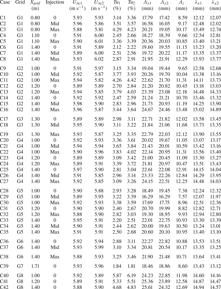
Table 3. Boundary-layer transition location ( $x_{ {\textit{tr}}}$) and averaged spanwise wavelength of the unsteady streamwise streaks ( $\lambda _z$) for cases C1–C42. Here $v_{\textit {rms}}/u_{\textit {rms}}$ and $w_{\textit {rms}}/u_{\textit {rms}}$ are anisotropy measures and $\mathit {Re}_{{\textit{FST}}}$ and $\mathit {Re}_{\Lambda }$ are free stream Reynolds numbers, all corresponding to leading-edge data. Indexes 1 and 2 represent hot-wire probes 1 and 2, respectively.

2.4. Method of transition location determination
The transition location is determined as the position where the intermittency factor ( $\gamma$) of the velocity signal is 0.5, which is halfway through the transition region. An intermittency factor of 0 and 1 correspond to a completely laminar and fully turbulent flow. The intermittency factor was calculated using the velocity-time signal acquired at the wall-normal location corresponding to the disturbance velocity peak inside the boundary layer (i.e. around $y \approx 1.3\delta _1$), using the method presented in Fransson et al. (Reference Fransson, Matsubara and Alfredsson2005). In figure 4, $\gamma$-distributions of grid G1 are shown for both increasing injection rate ( $a$) and decreasing $X_{{\textit{grid}}}$ ( $b$). In both cases, $Tu$ is increasing while $\Lambda _x$ is slightly decreasing. Dashed and dotted lines indicate the values of $\gamma = (0.1,0.5,0.9)$ and their intersection values with the $\gamma$-distribution where $\gamma = 0.5$, respectively. The latter being indicated with big square symbols and give locations of transition $x_{\textit{tr}} \equiv x_{\gamma = 0.5}$, from which the transitional Reynolds number ( $\mathit {Re}_{{\textit{tr}}}$) is calculated according to
 \begin{equation} \mathit{Re}_{{\textit{tr}}} = \frac{U_\infty x_{{\textit{tr}}}}{\nu}, \end{equation}
where  $U_\infty$ is measured at the leading edge. From these distributions, the transition region is defined for each case as ${\rm \Delta} x_{{\textit{tr}}} = x_{\gamma = 0.9}-x_{\gamma = 0.1}$. For improved accuracy of all $x$-location determinations ( $x_{\gamma = 0.1},x_{\gamma = 0.5},x_{\gamma = 0.9}$), a sigmoid curve was first fitted to the data in the least-square fit sense and then used as an analytical function to determine the $x$-locations. The curve fits are shown with solid lines in figure 4 and the $(+)$-symbols in ( $b$) are simply added to differentiate the symbols between injection and $X_ {\textit{grid}}$ changes.

Figure 3. Free-stream turbulence intensity decay ( $a$), and longitudinal integral length scale ( $b$) in the streamwise direction for cases C1–C42 in table 2. Here $X_{{\textit{grid}}}$ corresponds to the distance between the grid and the leading edge for each case, with the origin at the grid location. For symbol definitions, see table 1. The different streamwise evolution curves have been generated by changing $X_{{\textit{grid}}}$ and the injection rate for the active grids.

Figure 4. Streamwise intermittency factor distribution of grid G1. ( $a$) Effect of increasing the injection rate: (0, Mid, Max) as increased darkness of the symbols, which correspond to (C6, C7, C8), respectively. ( $b$) Effect of reducing $X_{{\textit{grid}}}$: (140, 110, 80) mm as increased darkness of the symbols, which correspond to (C6, C4, C1), respectively. See running text for lines and other symbols.
3. Boundary-layer streaks and laminar-turbulent transition
A well-cited result by Matsubara & Alfredsson (Reference Matsubara and Alfredsson2001) is that the averaged spanwise scale of the streaks asymptotes, with the downstream distance, to the value  $\lambda _z/2 \approx 3\delta _1$. Even if the result is right, it is unfortunate, since it often leads to the conclusion that no matter what the FST condition is, the same spanwise scale is eventually obtained. This is a puzzling result if one believes that the streaks are important for the transition and breakdown to the turbulence process. In this case, the FST characteristics should have an influence on the spanwise scale, since both $Tu$ and $\Lambda _x$ have an influence on the transition location. In this section new boundary-layer transition results are presented with a particular focus on a twofold effect of $\Lambda _x$ on the transition location (§ 3.1). It is also shown that the spanwise scale of the streaks is constant throughout the transition process and that the scale correlates with the FST condition (§ 3.2).
3.1. Transition region and location
The intermittency distribution derived by Johnson & Fashifar (Reference Johnson and Fashifar1994) has previously shown to agree well with experimental boundary-layer FST data (see, e.g., Fransson et al. Reference Fransson, Matsubara and Alfredsson2005). Their  $\gamma$-function, given as
 \begin{equation} \gamma (\xi)=1-{\mathrm{exp}}[-\mathcal{A}_1(\xi+\mathcal{A}_2)^{m}], \end{equation}
with  $m = 3$ from the derivation can be seen as a universal distribution since the experimental data closely falls on this curve independent of $Tu$ and $\Lambda _x$. Here, the dimensionless streamwise coordinate $\xi$ is defined as
 \begin{equation} \xi= \frac{x-x_{{\textit{tr}}}}{{\rm \Delta} x_{{\textit{tr}}}}, \end{equation}
where ‘tr’, in turn, was defined in § 2.4. Note also, that (3.1) is only valid in the range  $-A_2 \leq \xi < \infty$. For $\xi < -A_2$, the intermittency is per definition equal to zero since the flow is laminar upstream of the transition zone. In figure 5 all 84 intermittency distributions (from hotwires 1 and 2) are plotted versus $\xi$ and they all fall close to the dashed line corresponding to the universal $\gamma$-function, where the coefficients in (3.1) are the ones determined in the least square sense to the data in Fransson et al. (Reference Fransson, Matsubara and Alfredsson2005), i.e. $(\mathcal {A}_1,\mathcal {A}_2) = (0.60,1.05)$. The inset of figure 5 shows the same data in the dimensional streamwise coordinate $x$. This strengthens the universality of the distribution and serves as a consistency check between different data sets taken during different campaigns in different experimental set-ups. However, it is clear from the figure that the experimental distributions rises and flattens somewhat sharper than (3.1) (which also was the case in Fransson et al. Reference Fransson, Matsubara and Alfredsson2005), suggesting that the exponent $m$ is actually greater than 3 as derived by Johnson & Fashifar (Reference Johnson and Fashifar1994). Performing a straight forward unphysical least-square fit of (3.1) to the present data, by the inclusion of the exponent, gives $(\mathcal {A}_1,\mathcal {A}_2,m) = (0.023,1.87,5.47)$, which corresponds to the solid line in figure 5.

Figure 5. All 84 intermittency distributions from hot-wires 1 and 2 are shown in the scaled streamwise coordinate  $\xi$. Dashed and solid lines correspond to the Johnson & Fashifar (Reference Johnson and Fashifar1994) distribution and the best sigmoid curve fit to the data, respectively. The inset shows all intermittency distributions unscaled, filled and open symbols correspond to hot-wire probes 1 and 2, respectively.
In figure 6 the experimental intermittency distributions versus  $\xi$ are plotted for all different grids at 20 different spanwise locations, additionally confirming the universality of (3.1). To make the data accessible all boundary-layer transition results are collected for all FST conditions and summarized in table 3.

Figure 6. Streamwise intermittency distributions for all different grids spanning an averaged length of about  $9\delta _1$ in the spanwise direction. For symbols, see table 1.
The classical way to plot  $\mathit {Re}_{\textit {tr}}$ is versus $Tu$, which is known to have a strong influence on the transition location. However, as shown by Jonáš et al. (Reference Jonáš, Mazur and Uruba2000), $Re_{\textit {tr}}$ can change by a factor of 20 by changing the integral length scale of the FST while keeping $Tu$ constant at 3 %. Their result suggests that the integral length scale is of equal importance as $Tu$ when it comes to FST induced transition and, hence, the primary variable should be an FST parameter including both the velocity disturbance level and the integral length scale at the leading edge. Here, we will show that this parameter is an FST Reynolds number defined as
 \begin{equation} \mathit{Re}_{\textit{FST}} = \frac{u_{{\textit{rms}}} \Lambda_x}{\nu} = Tu \cdot \mathit{Re}_\Lambda, \end{equation}
where
 \begin{equation} \mathit{Re}_\Lambda = \frac{U_\infty \Lambda_x} {\nu}. \end{equation}
In figure 7(a) and (b) the transitional Reynolds number is plotted versus both  $Tu$ and $\mathit {Re}_{{\textit{FST}}}$, respectively. Using the physical reasoning by Andersson et al. (Reference Andersson, Berggren and Henningson1999), we can argue that the curve in figure 7(a) should have the form
 \begin{equation} (\mathit{Re}_{{\textit{tr}}})_{{\textit{cf}}}^{Tu} = \mathcal{B}_1 \cdot Tu^{-2} + \mathcal{B}_2, \end{equation}
where  $\mathcal {B}_1$ and $\mathcal {B}_2$ are constants and become $(\mathcal {B}_1,\mathcal {B}_2) = (148,31\,956)$ when least-square fitted to the data. Here $\mathcal {B}_2$ has been added, with the motivation of an existing minimum Reynolds number for self-sustained turbulence. The subscript ‘cf’ in (3.5) stands for an empirical curve fit to the present data and will be used throughout this paper. The same physical reasoning, based on input energy, as in Andersson et al. (Reference Andersson, Berggren and Henningson1999), can be used for the variable $\mathit {Re}_{\textit{FST}}$ and, hence, the curve in figure 7(b) corresponds to
 \begin{equation} (\mathit{Re}_{{\textit{tr}}})_{{\textit{cf}}} = \mathcal{C}_1 \cdot \mathit{Re}_{{\textit{FST}}}^{-2} + \mathcal{C}_2, \end{equation}
where  $\mathcal {C}_1$ and $\mathcal {C}_2$ are determined to $(\mathcal {C}_1,\mathcal {C}_2) = (7.6961\times 10^{9},62\,538)$. At first glance, the choice of $Tu$ seems to be the better option, since it collects the data points closer to the curve fitted line. However, plotting the data versus the primary variable $\mathit {Re}_{{\textit{FST}}}$ reorders the set of data in a favourable way, such that one can relate the deviation from the curve to the integral length scale through a scale-matching model, which will be introduced later. When comparing the values $\mathcal {B}_2$ with $\mathcal {C}_2$ one surprisingly realizes that they differ by a factor of 2 even though they should represent the same physical asymptotic value, i.e. a minimum $\mathit {Re}_{\textit {tr}}$ below which natural transition cannot take place. It becomes clear that $\mathcal {B}_2$ and $\mathcal {C}_2$ will only correspond to each other if additional data at much higher $Tu$ and $\mathit {Re}_{{\textit{FST}}}$ values are included in the fits.

Figure 7. Transitional Reynolds number, for all cases C1–C42 (HW1 and HW2), plotted versus  $Tu$ and $\mathit {Re}_{{\textit{FST}}}$ in ( $a$) and ( $b$), respectively.
The present data were collected with the mind of creating a large data set, which was done by changing both  $Tu$ and $\Lambda _x$ at the leading edge of the plate, without the effort in trying to change one of them independent of the other. However, there is enough data to group cases together with about the same $Tu$ but with different $\Lambda _x$. If one does that for different $Tu$ levels our data show that, for low turbulence intensities, the transition location moves upstream with increasing $\Lambda _x$ and downstream with increasing $\Lambda _x$ for high turbulence intensities. That is, there is a twofold effect of $\Lambda _x$ on the transition location, which confirms the findings reported both by Jonáš et al. (Reference Jonáš, Mazur and Uruba2000), Brandt et al. (Reference Brandt, Schlatter and Henningson2004), Ovchinnikov et al. (Reference Ovchinnikov, Piomelli and Choudhari2004) (of transition advancement) and Hislop (Reference Hislop1940) (of transition delay). The grouped cases are plotted in figure 8 with open symbols corresponding to the experiments and filled grey symbols to the corresponding predicted values that will be introduced and discussed later. The two trends will be explained by the fact that an optimal ratio between FST length scale and boundary-layer thickness at transition onset exists.

Figure 8. Twofold effect on  $\mathit {Re}_{\textit {tr}}$ by increasing $\Lambda _x$, while keeping $Tu$ close to constant. (a) For low $Tu~(\approx 2.16\,\%$ and 2.45 % $)$, transition moves upstream (i.e. $\mathit {Re}_{\textit {tr}}$ is reduced) for increasing $\Lambda _x$. (b) For high $Tu\ (\approx 2.82\,\%,\,3.37\,\%$ and 4.28 % $)$, transition moves downstream (i.e. $\mathit {Re}_{\textit {tr}}$ is increased) for increasing $\Lambda _x$. For symbols and cases, see tables 1 and 2, respectively. Here open symbols correspond to experimental data (from hot-wire 1) and filled grey symbols to predicted values.
3.2. Streamwise streaks inside the boundary layer
The asymptotic value of the spanwise length scale of the streamwise streaks is here argued not to be important for the transition process, in figure 11 of Matsubara & Alfredsson (Reference Matsubara and Alfredsson2001) the transition takes place farther upstream than the asymptotic limit in most cases, which makes the region where the data differs from each other the most interesting. This means that the cross-sectional aspect ratio of the streamwise structures at transition is such that the streaks are ovally shaped with the major axis being parallel with the surface. Now, the unsteady streamwise boundary-layer streaks, induced by the FST, can only be important for the transition location if their characteristic length scale correlates with the FST leading-edge parameters. The study by Fransson & Alfredsson (Reference Fransson and Alfredsson2003) supports the idea that the spanwise scale is set by the FST condition. In that study it was shown that by reducing the boundary-layer thickness by a factor of two, by means of creating an asymptotic suction boundary layer, the spanwise scale in the boundary layer remained the same, giving structures of an aspect ratio of two instead of one as suggested by the asymptotic limit  $\lambda _z/2 \approx 3\delta _1$ from Matsubara & Alfredsson (Reference Matsubara and Alfredsson2001).
In the present measurement campaign, two-point spanwise correlation measurements were performed at five different streamwise distances from the leading edge and at the location above the wall of maximum  $u_{\textit {rms}}$. These measurements were carried out at minimum and maximum injection when the grid was located at the closest and farthest downstream distances from the leading edge, resulting in 23 of the total 42 cases from tables 2 and 3. In figure 9 all measured spanwise correlation functions are plotted, where increasing darkness of the curves corresponds to increasing intermittency value. The spanwise distance $({\rm \Delta} z)$ between the two hot-wires where a negative minimum in $R_{uu} ({\rm \Delta} z)$ appears can be interpreted as the averaged half spanwise wavelength of the streaky structures $(\lambda _{z}/2)$. For each function, this minimum is consistently determined by a third-order polynomial fit to the data, and to obtain $\lambda _z$ for a specific intermittency value simple linear interpolation using the five streamwise locations is applied. Figure 10(a) shows $\lambda _z$ unscaled for $\gamma = 0.5$ versus its corresponding $Tu$ & $\Lambda _x$ and it shows that the data is scattered and uncorrelated with $Tu$ and $\Lambda _x$, it appears to be a range of possible $\lambda _z$ values for each $Tu$ and $\Lambda _x$. However, when scaled with the leading-edge FST condition using both $\Lambda _x$ and $Tu$, and plotted versus the primary variable $\mathit {Re}_{{\textit{FST}}}$ as in figure 10(b), the data fall close to a single curve. Here, the spanwise wavelength for $\gamma = 0.1$ has been added with filled square symbols, showing that the spanwise wavelength is constant throughout the transition region. The curve in figure 10(b) has been fitted to the data in the least-square fit sense, and implies that the averaged spanwise wavelength can be estimated from leading-edge FST parameters according to
 \begin{equation} \mathcal{L} = \Lambda_x \cdot Tu \left( \mathcal{D}_1 \cdot \mathit{Re}_{{\textit{FST}}}^{-1/\sqrt{2}} + \mathcal{D}_2 \right)^2, \end{equation}
with  $(\mathcal {D}_1,\mathcal {D}_2) = (186,0.8)$. That is, $\lambda _z$ is concluded to be correlated with the leading-edge FST parameters and, hence, to be an important length scale in the breakdown process to turbulence. From figure 10(c), it is clear that the estimated $\lambda _z$ using (3.7) stays within ${\pm }10\,\%$ of the measured value.

Figure 9. Two-point spanwise correlation functions for all measured distributions at different intermittency values. The colour bar shows the intermittency  $\gamma$.

Figure 10. Averaged spanwise wavelength of the streamwise streaks. Panels (a) and (b) show unscaled and scaled wavelengths versus  $Tu$ and $\Lambda _x$ and $\mathit {Re}_{{\textit{FST}}}$, respectively. Panel (c) indicates the accuracy in estimating $\lambda _z$ using (3.7) for different transitional Reynolds numbers. The solid lines correspond to deviations of ${\pm }10\,\%$ from the dashed line. Circular and square symbols correspond to streamwise locations of $\gamma = 0.5$ and 0.1, respectively.
Another evaluated quantity is the longitudinal integral length scale inside the boundary layer ( $\Lambda _{x}^{{\textit{BL}}}$, where ‘BL’ denotes boundary layer), which is a measure of how long the structures are in the streamwise direction. Here $\Lambda _{x}^{\textit {BL}}$ is calculated at the position above the wall corresponding to maximum $u_{\textit {rms}}$. Figure 11(a) shows streamwise $\Lambda _{x}^{\textit {BL}}$ distributions for all cases (see table 1 for symbols). The downstream distance is shown in $\xi$ and the colour brightness corresponds to the turbulence intensity at the leading edge, the darker the higher. A direct conclusion from this figure is that $\Lambda _{x}^{\textit {BL}}$ asymptotes to a constant value (just below 10 mm) in the turbulent region, i.e. for $\xi >2$. It is noteworthy that, regardless of the FST characteristics, the streamwise length scale will eventually be the same, i.e. there is no memory of the initial FST condition in the turbulent region. From the location where the unsteady streaks are created, they will grow in the streamwise direction becoming longer until around $\xi = -0.5$, i.e. around the onset of transition where $\gamma$ is close to 0.10. After this location, the streaks become shorter due to the appearance of turbulent spots and asymptotes to the constant value. The maximum value of $\Lambda _{x}^{\textit {BL}}$ (around $\xi = -0.5$) is plotted in figure 11(b). No satisfactory correlation function was found with $\mathit {Re}_{{\textit{FST}}}$ as the primary variable as was found for a dimensionless $\lambda _z$ (cf. figure 10b), but there is a clear trend of shorter streaks as $\mathit {Re}_{{\textit{FST}}}$ is increased. Instead, in figure 11(c) $\Lambda _{x,\textit {max}}^{\textit {BL}}$ is normalized with $\mathcal {L}$ (3.7) and $Tu$, which makes the data points fall close to a straight line when plotted against $\mathit {Re}_{\textit {tr}}$. The length scale ratio ( $\Lambda _{x,\textit {max}}^{\textit {BL}} / \mathcal {L}$) corresponds to the streamwise/spanwise aspect ratio at the maximum streak length and can be estimated from known inlet FST conditions as
 \begin{equation} \left( \frac{\Lambda_{x,{\textit{max}}}^{{\textit{BL}}}}{\mathcal{L}} \right) = Tu \cdot \left( \mathcal{E}_1\,\mathit{Re}_{{\textit{tr}}} + \mathcal{E}_2 \right), \end{equation}
where  $(\mathcal {E}_1,\mathcal {E}_2) = (5.293 \times 10^{-4},-15.75)$ corresponding to the straight line in figure 11(c). The missing parameter to assess the aspect ratio is the parameter $\mathit {Re}_{\textit {tr}}$, which can be predicted for the given leading-edge FST parameters $\mathit {Re}_{{\textit{FST}}}$ and $Re_\Lambda$, as will be shown in § 4.

Figure 11. (a) Streamwise distribution of the integral length scale inside the boundary layer ( $\Lambda _{x}^{\textit {BL}}$) versus the non-dimensional transition coordinate $\xi$. The brightness of the symbols illustrates the turbulence intensity, with darker colours corresponding to higher $Tu$. (b) Maximum values of $\Lambda _{x}^{\textit {BL}}$ for each distribution in (a) versus its corresponding $\mathit {Re}_{{\textit{FST}}}$. Panel (c) indicates a linear correlation between appropriately scaled $\Lambda _{x,\textit {max}}^{\textit {BL}}$ and the transitional Reynolds number.
4. A semi-empirical transition prediction model
Recent results have shown a clear dependence of  $\Lambda _x$ on the transition location, moving the transition location upstream with increasing $\Lambda _x$. The present results confirm this result but also show that the transition location can move downstream with increasing $\Lambda _x$, in agreement with earlier results by Hislop (Reference Hislop1940). That is, the effect of $\Lambda _x$ can be twofold. There are numerous simple empirical correlation functions available that have been published over the years, based on different experimental data sets, but none of them includes $\Lambda _x$ in a way such that the twofold effect can be predicted. The existing experimental data, taken in the same experimental set-up under the same conditions, using the same transition determination method, has so far been too scarce and not enough to find the appropriate behaviour of $\Lambda _x$ when other parameters such as $Tu$ and the vertical boundary-layer scale (i.e. $U_\infty$) are varied.
Apart from the leading-edge FST parameters  $\Lambda _x$ (2.1), $\mathit {Re}_{{\textit{FST}}}$ (3.3) and $\mathit {Re}_\Lambda$ (3.4), where the latter two are related to each other via $Tu$ (2.2), there is another important parameter that provides the missing link to the boundary layer, namely the vertical boundary-layer length scale,
 \begin{equation} \delta_{{\textit{tr}}} = \sqrt{\frac{\nu x_{\textit{tr}}}{U_\infty}}, \end{equation}
at transition. The only shortcoming is that this parameter includes  $x_{\textit {tr}}$, which is the one that is in demand.
4.1. Scale-matching model
The present experimental data indicates that there is a change of trend of the influence of  $\Lambda _x$ on the transitional Reynolds number. This information suggests that a scale matching between the FST and the boundary layer has to take place at the trend change. The local integral length scale of the FST, which grows with the square root of the downstream distance, is proportional to the integral length scale at the leading edge (see, e.g., Kurian& Fransson (Reference Kurian and Fransson2009), or the present figure 3b) which in turn suggests that the ratio $\Lambda _x / \delta _{\textit{tr}}$ is important for where the transition happens. Here, the following hypothesis is formulated.
Hypothesis.For a given  $Tu$, there is an optimal scale ratio $(\Lambda _x / \delta _{\textit{tr}})_\textit {opt}$that promotes transition. The transitional Reynolds number versus the scale ratio has a minimum at the optimal scale ratio. A mismatch from the optimal value will give a negative derivative of $\mathit {Re}_{\textit {tr}}$, with respect to the scale ratio, if the scale ratio is lower than the optimal, and a positive derivative if it is larger.
This hypothesis was first formulated in Fransson (Reference Fransson2017), but there with the scale ratio inverted. A sketch is shown in figure 12, where the curves correspond to a specific  $Tu$ value. The higher the $Tu$, the closer the curve is to the abscissa. To confirm the hypothesis new experiments at constant $Tu$ with varying $\Lambda _x$ need to be carried out, the present database is not sufficient since both $Tu$ and $\Lambda _x$ were varied. However, the present data seem to indicate that $(\Lambda _x / \delta _{\textit{tr}})_\textit {opt}$ is close to 15, which would imply that the change of trend appears where $\Lambda _x$ is about three times the boundary-layer thickness, i.e. $\delta _\mathrm {99}$, at transition. This means that if $\Lambda _x < 3\,\delta _{99}$ at transition, the transition location is expected to move upstream, and vice versa, with increasing $\Lambda _x$.

Figure 12. Sketch shows the scale-matching model, based on the hypothesis that, for each  $Tu$, there exists an optimal $\Lambda _x/\delta _{\textit {tr}}$ that promotes transition to a lowest possible $\mathit {Re}_{\textit {tr}}$.
4.2. The equation for the transitional Reynolds number
The effect of  $\Lambda _x / \delta _{\textit{tr}}$ on $Re_{\textit {tr}}$ is assumed to enter as a correction to (3.6) and, hence, we make the following ansatz:
 \begin{equation} \mathit{Re}_{{\textit{tr}}} = (\mathit{Re}_{{\textit{tr}}})_{{\textit{cf}}} + {\rm \Delta} \mathit{Re}_{{\textit{tr}}}, \end{equation}
where
 \begin{equation} {\rm \Delta} \mathit{Re}_{{\textit{tr}}} = {\rm \Delta} \mathit{Re}_{{\textit{tr}}}(\Lambda_x/\delta_{{\textit{tr}}}), \end{equation}
i.e. we assume that the correction term  ${\rm \Delta} \mathit {Re}_{\textit {tr}}$ can be written as a function of the scale ratio, as derived below. If the scale ratio is matched with the one corresponding to the curve of (3.6), ${\rm \Delta} \mathit {Re}_{\textit {tr}}$ will give a zero contribution. On the other hand, the more the scale ratio deviates from the one corresponding to the curve (3.6), the larger the correction becomes. To amplify the sensitivity of the scale ratio, the square of this ratio is introduced in the correction as
 \begin{equation} {\rm \Delta} \mathit{Re}_{{\textit{tr}}} = \kappa\left[ \left( \frac{\Lambda_x}{\delta_{{\textit{tr}}}} \right)^2 - \left( \frac{\Lambda_x}{\delta_{{\textit{tr}}}} \right)^2_{{\textit{cf}}} \right], \end{equation}
where
 \begin{equation} \left( \frac{\Lambda_x}{\delta_{{\textit{tr}}}} \right)^2 \equiv \left( \frac{\mathit{Re}_{{\textit{FST}}}}{Tu} \right)^2 \frac{1}{\mathit{Re}_{{\textit{tr}}}}, \end{equation}
and  $\kappa$ is a weighting function. Furthermore, by making the above choice of introducing the correction with the square of the scale ratio will simplify the final equation. In analogy with (4.5) we then introduce $( \Lambda _x / \delta _{\textit {tr}} )^2_{\textit{cf}}$ in (4.4) as
 \begin{equation} \left( \frac{\Lambda_x}{\delta_{{\textit{tr}}}} \right)^2_{\textit{cf}} = \left( \frac{\mathit{Re}_{{\textit{FST}}}}{Tu} \right)^2 \frac{1}{( \mathit{Re}_{{\textit{tr}}})_{{\textit{cf}}}}. \end{equation}
Now, by combining (4.2) and (4.4)–(4.6), and multiplying with  $\mathit {Re}_{\textit {tr}}$ the following second-order equation of $\mathit {Re}_{\textit {tr}}$ can readily be derived:
 \begin{equation} \mathit{Re}_{{\textit{tr}}}^2 +\underbrace{ \left[ \kappa\,\mathit{Re}_\Lambda^2 \frac{1}{(\mathit{Re}_{{\textit{tr}}})_{{\textit{cf}}}} - ( \mathit{Re}_{{\textit{tr}}})_{{\textit{cf}}} \right] }_{ = \, \alpha}\, \mathit{Re}_{{\textit{tr}}}~- \underbrace{\kappa\,\mathit{Re}_\Lambda^2}_{= \, \beta} = 0, \end{equation}
with the solution
 \begin{equation} \mathit{Re}_{{\textit{tr}}} = -\frac{\alpha}{2} \pm \sqrt{\left( \frac{\alpha}{2} \right)^2 + \beta}. \end{equation}
When the scale ratio  $(\Lambda _x / \delta _{\textit {tr}})^2$ corresponds to (4.6), the Reynolds number correction (4.4) is zero and the solution is a double root corresponding to $\mathit {Re}_{\textit {tr}} = (\mathit {Re}_{\textit {tr}})_{{\textit{cf}}}$ (cf. 3.6). If there is a mismatch of the scale ratio with respect to (4.6), there will be two different roots, namely (3.6) and (4.2), which is given by (4.8). Finally, we note that both $\alpha$ and $\beta$ depend on the parameter $\mathit {Re}_\Lambda$ and the weighting function $\kappa$. While $\mathit {Re}_\Lambda$ is considered known from the FST condition at the leading edge, $\kappa$ requires further analysis.
4.3. Weighting function
The weighting function  $\kappa$ is introduced in (4.4) and corresponds to
 \begin{equation} \kappa = \frac{{\rm \Delta} \mathit{Re}_{{\textit{tr}}}}{\left[ \left( \Lambda_x / \delta_{{\textit{tr}}} \right)^2 - \left( \Lambda_x /\delta_{{\textit{tr}}} \right)^2_{{\textit{cf}}} \right]}, \end{equation}
which may be rewritten using (4.5), (4.6) and (3.3) to
 \begin{equation} \kappa = - \mathit{Re}_\Lambda^{-2}\,\mathit{Re}_{{\textit{tr}}} \cdot ( \mathit{Re}_{{\textit{tr}}})_{\textit{cf}} < 0. \end{equation}
This expression of  $\kappa$ needs to be modelled since it includes $\mathit {Re}_{\textit {tr}}$ and renders a trivial solution when inserted to (4.7). Besides, it is noted that $\kappa$ is always negative. For the modelling, $\kappa$ is plotted versus $\mathit {Re}_{{\textit{FST}}}$ in figure 13(a) using the experimental data and (3.6). The model function should have two constraints for an accurate representation, in the limits of $\mathit {Re}_ {\textit{FST}} \rightarrow 0$ and $\mathit {Re}_{\textit{FST}} \rightarrow \infty$ the function should approach zero. The physical reasoning behind this is that ${\rm \Delta} \mathit {Re}_{\textit {tr}}$ should approach zero in these two limits. For $\mathit {Re}_{\textit{FST}} \rightarrow \infty$, the transitional Reynolds number will approach the minimum Reynolds number for self-sustained turbulence (cf. $\mathcal {B}_1$ in (3.6)) and the dependence of $\Lambda _x$ will diminish. For $\mathit {Re}_{\textit{FST}} \rightarrow 0$, the FST transition scenario will eventually be replaced by the T–S wave transition scenario and the effect of $\Lambda _x$ is expected to disappear. However, it is worth pointing out that independent of an accurate representation of $\kappa$ the transition prediction model described by (4.7) is only valid for the transition scenario dominated by FST. Here, the $\kappa$ function is created in order to fulfil the above constraints with a good fit to the data according to
 \begin{equation} \kappa = -10^3 \times \left[\underbrace{\frac{{G} \cdot \mathit{Re}_{ {\textit{FST}}}}{a + \vert\,(\mathit{Re}_{{\textit{FST}}} - a)^b\,\vert }}_{= f_1} + \underbrace{c\cdot \exp\{ -d(\mathit{Re}_{{\textit{FST}}}-e)^2 \} }_{= f_2} \right]^2. \end{equation}
The five coefficients ( $a$–
$a$– $e$) are determined in the least-square fit to the data and ${G}$ is set to ${G} = 25$, which is the gain to $f_1$ and chosen such that the turnaround of $\kappa$ to fulfil the constraint in the limit for $Re_{{\textit{FST}}} \rightarrow 0$ is around $\mathit {Re}_{{\textit{FST}}} = 73$. This value of $\mathit {Re}_{{\textit{FST}}}$ corresponds to $Tu = 1\,\%$, which is obtained through the relation
 \begin{equation} \mathit{Re}_{{\textit{FST}}} = \left(\frac{\mathcal{B}_1 \cdot Tu^{-2} + \mathcal{B}_2 - \mathcal{C}_2}{\mathcal{C}_1}\right)^{-1/2}, \end{equation}
derived by combining (3.5) and (3.6). The value of  $Tu \approx 1$ % is often used as a threshold from where the transition scenario is dominated by the growth and breakdown of unsteady streamwise streaks (see, e.g., Arnal & Juillen Reference Arnal and Juillen1978). The five coefficients in (4.11) are determined to be
 \begin{align} \begin{aligned} a &= 7.2279 \times 10^1;\quad b = 1.7574 \times 10^0;\quad c = 3.9519 \times 10^{-2}; \nonumber\\ d &= 5.6340 \times 10^{-5};\quad e = 3.1987 \times 10^2. \end{aligned} \end{align}
In figure 13(a) both parts,  $f_1$ and $f_2$, in (4.11) are plotted and it is clear that the sum of the two gives a satisfactory fit to the data. Figure 13(b) shows the full $\kappa$ function. The grey areas in figure 13 indicate $\mathit {Re}_{{\textit{FST}}}$ values being lower than $Tu = 1\,\%$. On the one hand, there are too few data points at low $\mathit {Re}_{{\textit{FST}}}$ to comment on the behaviour of $\kappa$ in the lower range of $\mathit {Re}_{{\textit{FST}}}$, on the other hand, the data do indicate that the effect of $\Lambda _x$ on $Re_{\textit {tr}}$ only becomes greater as $\mathit {Re}_{{\textit{FST}}}$ is reduced. The physical constraint that the effect of $\Lambda _x$ eventually has to diminish as $\mathit {Re}_{\textit {tr}} \rightarrow 0$ gives rise to the sharp turnaround of the function.

Figure 13. Weighting function  $\kappa$ versus $\mathit {Re}_{{\textit{FST}}}$. (a) Close up of the $\kappa$-function according to (4.10), symbols correspond to experimental data. (b) Full $\kappa$-function produced by (4.10) for the range $\mathit {Re}_{{\textit{FST}}} = 0\text {--}700$. Grey regions correspond to $\mathit {Re}_{{\textit{FST}}} \leq 73$, which by combining (3.5) and (3.6) leads to $Tu \leq 1\,\%$.
5. Validation of the model
Figure 14 shows a direct comparison between the experimental and predicted  $\mathit {Re}_{\textit {tr}}$ as a function of $\mathit {Re}_\Lambda$ and $Tu$. Noteworthy is that the only input to the model is leading-edge data with two out of the following three FST parameters: $\mathit {Re}_\Lambda$, $Tu$ and $\mathit {Re}_{{\textit{FST}}}$ (which are related to each other in (3.3)). Practically, the model requires a single-point time-resolved velocity measurement in the free stream at the leading edge. Quantitatively, the agreement is satisfactory between figures 14(a) and 14(b). The circular symbols correspond to the actual input FST data, where the corresponding measured or predicted $\mathit {Re}_{\textit {tr}}$ are used to produce the contour plots. Even though figure 14(a) shows a quite complex behaviour of $\mathit {Re}_{\textit {tr}}$ with a clear dependence on both $Tu$ and $\Lambda _x$, our semi-empirical model clearly captures the essential physics with the introduced scale-matching model, which links the FST to the boundary layer.

Figure 14. Contour plots of the transitional Reynolds number. (a) Experimental data. (b) Predicted data by (4.7). Circular symbols indicate measured cases in the  $\mathit {Re}_\Lambda$– $Tu$ plane.
In figure 15 a qualitative comparison between experimental and predicted  $\mathit {Re}_{\textit {tr}}$ values is made. From figure 15(a), it is clear that (4.7) performs very well for $\mathit {Re}_{{\textit{FST}}}>325$, while in the range below 325 one may foresee improvements given more experimental data in the future to tune the model. However, one may conclude that the model does significantly better than simple empirical correlations based on only $\mathit {Re}_{{\textit{FST}}}$ or $Tu$, which completely excludes the effect of $\Lambda _x$ on $\mathit {Re}_{\textit {tr}}$. Figure 15(b) quantifies this statement, by showing that the predicted value using the scale-matching model (4.7) is significantly improved with respect to the usage of (3.6). Using (4.7) for predicting the transitional Reynolds number gives 65 % of the values within ${\pm } 10$ % of the experimental data, while (3.6) gives 40 % within ${\pm } 10$ %. Less than 10 % of the data is outside ${\pm } 20$ % using (4.7), while (3.6) gives 31 % of the data worse than ${\pm } 20$ %. Figure 16 shows a classical scatter plot of the same data as shown in figure 15(b) with the corresponding ${R}^2$ coefficients given in the caption.

Figure 15. (a) Qualitative comparison between the measured transitional Reynolds number (open circles) and the corresponding predicted values (black circles) versus  $Re_{{\textit{FST}}}$. The solid line corresponds to (3.6). (b) Predicted values with respect to the measured values, from (4.7) and (3.6) with black square symbols and open squares, respectively.


At last, we turn our attention back to figure 8, where the effect of  $\Lambda _x$ on $\mathit {Re}_{\textit {tr}}$ was illustrated for five different $Tu$ levels. The grey symbols in this figure correspond to the predicted $\mathit {Re}_{\textit {tr}}$ using (4.7) and again a qualitative comparison is made but with the specific cases denoted in the figure. From this comparison, it is confirmed that the prediction is better for higher $\mathit {Re}_{{\textit{FST}}}$ values (i.e. in general for higher $Tu$), as shown in figure 8(b). However, it is also clear that the twofold effect of $\Lambda _x$ on $\mathit {Re}_{\textit {tr}}$ is captured by the model, even though the influence of $\Lambda _x$ is slightly underpredicted for low $Tu$ values (cf. figure 8a). Going back to the scale-matching hypothesis (figure 12) it is also clear that if one does not accurately capture $(\Lambda _x / \delta _{\textit {tr}})_\textit {opt}$ from the data when tuning the model it is easy to underpredict or overpredict the influence of $\Lambda _x$. From figure 8, it seems that the behaviour for low $Tu$ levels would be predicted even better if the curve in the sketch (cf. figure 12) was shifted to the right. Now, with this information at hand, having data taken under constant $Tu$ levels while varying $\Lambda _x$ instead of scattered data in the $(\mathit {Re}_\Lambda ,\,Tu)$ plane (as the present data), would be valuable for future tuning of the model.
In figure 17 the semi-empirical model (4.7) has been used to produce the contour plots of  $\mathit {Re}_{\textit {tr}}$ in (a) and (b), where contour lines have been added of constant $\mathit {Re}_{{\textit{FST}}}$ and $Tu$, respectively. While figure 17(a) is similar to figure 14 but plotted for a somewhat extended range of $\mathit {Re}_\Lambda$ and $Tu$, figure 17(b) shows $\mathit {Re}_{\textit {tr}}$ predicted in the $\mathit {Re}_\Lambda$– $\mathit {Re}_{{\textit{FST}}}$ plane. Since the behaviour of $\Lambda _x$ on $\mathit {Re}_{\textit {tr}}$ has so far not been known, except for the $\Lambda _x$ variation for a particular $Tu$ level that has been published (see, e.g., Jonáš et al. Reference Jonáš, Mazur and Uruba2000), the figures 17(a) and 17(b) are the first ones ever produced for a larger variable range showing how $\mathit {Re}_{\textit {tr}}$ is affected by the FST condition based on the present experimental data.

Figure 17. Contour plots of predicted transitional Reynolds numbers by (4.7). (a)  $\mathit {Re}_\Lambda$– $Tu$ plane, with contour lines corresponding to $\mathit {Re}_{{\textit{FST}}} = 100{:}100{:}700$, from left to right. (b) $\mathit {Re}_\Lambda$– $\mathit {Re}_{{\textit{FST}}}$ plane, with contour lines corresponding to $Tu = 0.01{:}0.01{:}0.07$, from left to right.
6. Conclusion
Ideally, we would like to be able to predict the transition location in a boundary layer with the only knowledge being the leading-edge FST condition. However, today no simple correlation function exists that includes the effect of FST length scales on transition in a physically correct way. The underlying problem is that none of the existing prediction functions, so far, links the FST condition to the boundary layer. Reviewing the existing literature on the effect of FST length scales one finds that the FST integral length scale has a twofold effect on transition, i.e. an increase of  $\Lambda _x$ can both lead to advancement and delay in transition. It is obvious that empirical correlation functions only including the turbulence intensity, as most past empirical relations, and that relations with a linear $\Lambda _x$ dependence, as more recent published relations, will do a poor job in predicting the transition.
Here, we present data from a large wind tunnel campaign aimed at bringing further insights to the FST induced boundary-layer transition scenario. It is a zero-pressure gradient boundary layer subject to different FST conditions at the leading edge that is in focus. The FST was varied by means of eight different turbulence generating grids of different mesh and bar widths. Six of these grids were active in the sense of having upstream injected jets of high speed to increase the pressure drop over the grids, which in turn increases  $Tu$. In total, data from 42 unique FST conditions have been acquired and documented in the present paper (cf. tables 2 and 3). The FST is known to create unsteady elongated streamwise streaks of alternating high- and low-speed regions inside the boundary layer, via some receptivity mechanism which takes place already at the leading edge. The averaged spanwise wavelength of these structures is likely to be set already in the leading-edge region and to be critical for the breakdown to turbulence process.
Our data confirm the previously reported universal intermittency distribution when the non-dimensional streamwise coordinate  $\xi$ is used (cf. figure 5). This distribution as a function of the dimensional streamwise coordinate, $x$, is used to determine the transition location for each case. Here, $x_{\textit {tr}}$ is consistently determined as to where the intermittency factor of the velocity signal is equal to 0.5 (measured around the $u_{\textit {rms}}$ peak above the plate).
The present dataset is the first one indicating the twofold effect of  $\Lambda _x$ in the same experimental set-up and campaign. On the one hand, it is shown that by increasing $\Lambda _x$ by 12 % the transitional Reynolds number is reduced by 38 % at $Tu \approx 2.16\,\%$ (from case C6 to C33). On the other hand, an 18 % increase of $\Lambda _x$ at $Tu \approx 2.82\,\%$ results in an increase of $Re_{\textit {tr}}$ by 45 % (from case C32 to C25).
To characterize the FST condition we establish three FST parameters, namely  $\mathit {Re}_{{\textit{FST}}}$, $\mathit {Re}_\Lambda$ and $Tu$, which are all related to each other (cf. (3.3)). By introducing a scale-matching model the physically correct behaviour of $\Lambda _x$ on $\mathit {Re}_{\textit {tr}}$ can be obtained. In this analysis the primary variable in predicting $\mathit {Re}_{\textit {tr}}$ turns out to be $\mathit {Re}_{{\textit{FST}}}$ and not $Tu$, as used in most correlation functions. Dealing with the data as a function of $\mathit {Re}_{{\textit{FST}}}$ completely reorders the data and allows for the introduction of a ${\rm \Delta} \mathit {Re}_{\textit {tr}}$ (4.2)–(4.4), which is a function of the scale ratio $\Lambda _x / \delta _{\textit {tr}}$ that links the FST length scale with the boundary layer. A similar analysis with $Tu$ as the primary variable was carried out, but without success. The key ingredient in being able to predict $\mathit {Re}_{\textit {tr}}$ is the scale-matching model, which leads to a second-order equation of $\mathit {Re}_{\textit {tr}}$ with $\mathit {Re}_{{\textit{FST}}}$ being the primary variable and $\mathit {Re}_\Lambda$ being a parameter in the equation (cf. (4.7)). This equation captures the twofold behaviour of $\Lambda _x$ on $\mathit {Re}_{\textit {tr}}$, and gives a significantly improved prediction of $\mathit {Re}_{\textit {tr}}$ with respect to a single variable prediction, be it $\mathit {Re}_{{\textit{FST}}}$ or $Tu$. The scale-matching hypothesis leads to the threshold of $(\Lambda _x / \delta _{\textit {tr}})_\textit {opt}$ and the data suggest that this value is close to 15, which in turn leads to the conclusion that when $\Lambda _x < 3\delta _{99}$ at transition, the transition location will move upstream, and vice versa, with increasing $\Lambda _x$.
The data also indicate that both the averaged spanwise wavelength of the streaks,  $\lambda _z$, as well as the maximum streamwise length of the unsteady streaks, $\Lambda _{x,{\textit {max}}}^{\textit {BL}}$, correlate with the FST parameters. This finding is important since quite often the streak spacing is said to adapt to the boundary-layer thickness giving structures of an aspect ratio of one inside the boundary layer (after Matsubara & Alfredsson Reference Matsubara and Alfredsson2001), which can be used to diminish the role of the streaks in the transition process. Here, we argue that the asymptotic aspect ratio of the streaks, after the adaptation, is not important for the transition, since for most cases (moderate to high $Tu$ levels) transition occurs upstream of this asymptotic state.
Our data show that  $\lambda _z$ is proportional to both $\Lambda _x$ and $Tu$, with the correlation function being a function of $\mathit {Re}_{{\textit{FST}}}$ (cf. (3.7)). The maximum streamwise extent of the streaks (around $\gamma = 0.1$), $\Lambda _{x,{\textit {max}}}^{\textit {BL}}$, is proportional to $\Lambda _x$, $Tu^2$ and $\mathit {Re}_{\textit {tr}}$, which implies that the transition location needs to be estimated before the streamwise length of the streaks can be estimated (cf. (3.8)). These length scales are believed to be important for the streak instability. In particular, the former length scale, which together with the streak amplitude gives a measure of the spanwise velocity gradient that drives the sinusoidal secondary instability. Here, believed to be the most common precursor to the local breakdown into turbulent spots inside the boundary layer. With this in mind, it is also likely that a universal transitional number based on local flow properties inside the boundary layer exists, which so far has not been recognized.
Finally, the semi-empirical transition prediction model presented herein captures the twofold effect of  $\Lambda _x$ on $\mathit {Re}_{\textit {tr}}$ in a correct way, and we can, for the first time, get the full behaviour of $\mathit {Re}_{\textit {tr}}$ in the $Tu$–
$Tu$– $\mathit {Re}_\Lambda$ and $\mathit {Re}_{{\textit{FST}}}$– $\mathit {Re}_\Lambda$ planes based on the model. Theoretically, one would only need to perform a single-point time-resolved velocity measurement in the free stream at the leading edge in order to predict the transition location using the new model. From this velocity signal, $U_\infty$, $u_{\textit {rms}}$ and $\Lambda _x$ can be obtained, which are required for calculating the non-dimensional FST parameters $\mathit {Re}_{{\textit{FST}}}$, $\mathit {Re}_\Lambda$ and $Tu$. In reality, there is primarily one additional parameter that plays a role for the transition location, namely the leading-edge pressure gradient, which apart from the leading-edge geometry is given by the leading-edge stagnation line. However, with increasing turbulence intensity the leading-edge pressure gradient effect is expected to diminish. Other parameters related to the wind tunnel set-up, such as plate joints and background acoustic noise are not expected to play a significant role as long as joints are kept smooth without steps. Acoustic noise can interact with the leading edge and two-dimensional plate joints to generate T–S waves but is only expected to play a role when the turbulence intensity is very low (i.e. $Tu \ll 1$ %). For moderate to high turbulence intensities, the T–S waves are likely to be damped by the unsteady streamwise streaks and can be considered harmless for the transition since the scenario is dominated by the growth of streamwise streaks. The present authors believe that the two most important reasons for the large discrepancy of experimental data acquired in different facilities, when it comes to $\mathit {Re}_{\textit {tr}} = \mathit {Re}_{\textit {tr}}(Tu)$, are as follows: (1) different methods in determining the transition location; and (2) past lack of knowledge regarding the significance of ${\Lambda _x}$ on the transition location.
Acknowledgments
The Swedish Research Council and the Swedish Foundation for Strategic Research are acknowledged for their financial support of the projects EXCALIBUR 2015-04714 and TRANSaCT SM16–0007, respectively.
Declaration of interests
The authors report no conflict of interest.


 Open access