


1 Introduction
The study of the transition to turbulence usually starts with the investigation of the linear instabilities of the laminar solution. Plane Poiseuille flow (PPf), the solution of channel flow with a parabolic profile, is one of the few analytical solutions of the Navier–Stokes equations. Its stability has been studied extensively, with the ambition to predict the transition to turbulence in this simple flow geometry. This solution loses its stability in favour of two-dimensional Tollmien–Schlichting (TS) waves at  $Re=5772$, where the Reynolds number $Re=U_{cl}h/\unicode[STIX]{x1D708}$ is based on $U_{cl}$ – the centreline velocity of the corresponding Poiseuille flow solution, $h$ – the half-gap, and $\unicode[STIX]{x1D708}$ – the kinematic viscosity of the fluid (Orszag Reference Orszag1971). Turbulence, however, is already found in channel experiments at $Re=1000$ and below. Although the TS instability is subcritical in $Re$, (Stuart Reference Stuart1960; Ehrenstein & Koch Reference Ehrenstein and Koch1991) the bifurcated branches fail to reach the low values of $Re$ where the onset of turbulence is reported in early transition experiments (Carlson, Widnall & Peeters Reference Carlson, Widnall and Peeters1982; Nishioka & Asai Reference Nishioka and Asai1985; Alavyoon, Henningson & Alfredsson Reference Alavyoon, Henningson and Alfredsson1986; Klingmann Reference Klingmann1992; Seki & Matsubara Reference Seki and Matsubara2012; Lemoult, Aider & Wesfreid Reference Lemoult, Aider and Wesfreid2013). More critically, the TS waves, having only spanwise vorticity, bear little structural resemblance with the coherent structures observed in the corresponding turbulent regimes, which are characterised by quasi-streamwise streaks and vortices.
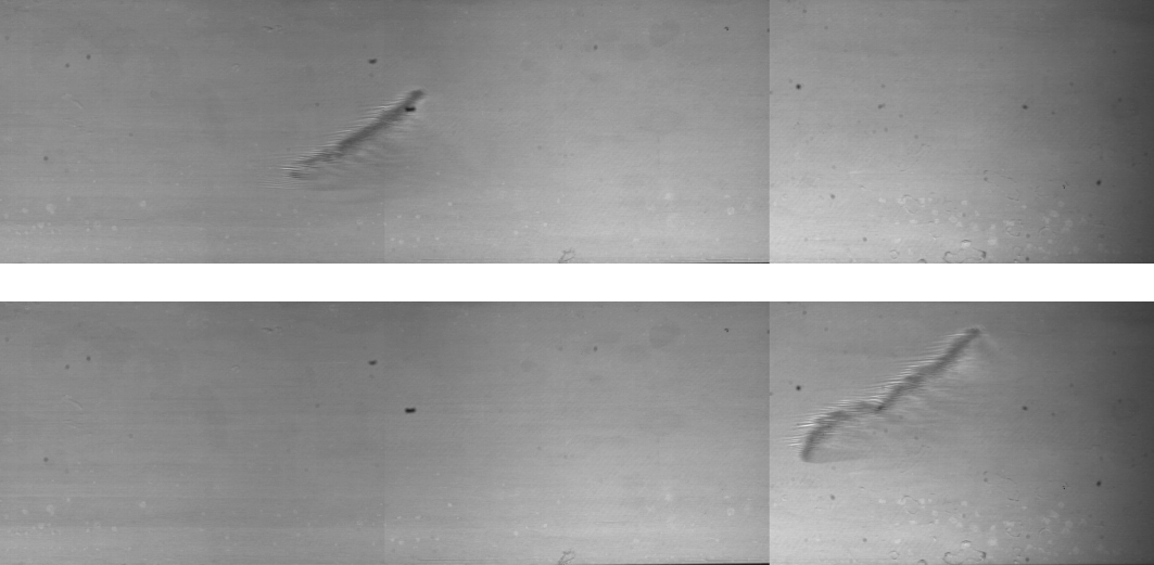
Figure 1. Experimental observation of an elongating isolated oblique stripe at  $Re=700$ in a water channel as it travels downstream. The flow is from the left to the right. Reflective mica particles were added for visualisation.
From the analysis of the self-sustaining process of turbulence (Hamilton, Kim & Waleffe Reference Hamilton, Kim and Waleffe1995), it has become clear that different solutions of the governing Navier–Stokes equations ought to exist, which capture key components of turbulent flows and are more relevant to the transition process (Jiménez et al. Reference Jiménez, Kawahara, Simens, Nagata and Shiba2005; Kawahara, Uhlmann & Van Veen Reference Kawahara, Uhlmann and Van Veen2012). The first solutions were identified as steady states in plane Couette flow by Nagata (Reference Nagata1990), followed by many others (see e.g. Gibson, Halcrow & Cvitanović (Reference Gibson, Halcrow and Cvitanović2009)). Many solutions have been found in other shear flow geometries in the form of travelling waves (TWs), see Waleffe (Reference Waleffe2001), Nagata & Deguchi (Reference Nagata and Deguchi2013), Park & Graham (Reference Park and Graham2015), Neelavara, Duguet & Lusseyran (Reference Neelavara, Duguet and Lusseyran2017), Wall & Nagata (Reference Wall and Nagata2016) in the context of channel flow and Faisst & Eckhardt (Reference Faisst and Eckhardt2003), Wedin & Kerswell (Reference Wedin and Kerswell2004) for pipe flow. They are disconnected from the laminar profile and all are linearly unstable. The entanglement of their stable and unstable manifolds has been conjectured to form a deterministic backbone for the low- $Re$ turbulent dynamics (Kawahara et al. Reference Kawahara, Uhlmann and Van Veen2012). Many of these studies were performed in small periodic domains. Though conceptually useful, these studies are motivated by higher $Re$ wall turbulence studies (Jiménez & Moin Reference Jiménez and Moin1991) and turn out to be inadequate to capture crucial characteristics of lower $Re$ turbulent flows, such as spatial localisation. Indeed, ample experimental and numerical evidence from studies in large domains show that wall-bounded turbulence at the lowest possible values of $Re$ remains localised. Besides, the corresponding laminar–turbulent interfaces display non-zero angles with respect to the laminar flow direction (Coles Reference Coles1965; Prigent et al. Reference Prigent, Grégoire, Chaté, Dauchot and van Saarloos2002; Tsukahara et al. Reference Tsukahara, Seki, Kawamura and Tochio2005; Hashimoto et al. Reference Hashimoto, Hasobe, Tsukahara, Kawaguchi and Kawamura2009; Duguet, Schlatter & Henningson Reference Duguet, Schlatter and Henningson2010; Fukudome & Iida Reference Fukudome and Iida2012; Xiong et al. Reference Xiong, Tao, Chen and Brandt2015). Starting from fully turbulent flow, as $Re$ is decreased, criss-cross stripe patterns appear. As $Re$ is decreased further, the mean spacing between these stripes of turbulence increases, to the extent that they appear isolated in an otherwise laminar environment (see Tsukahara & Ishida (Reference Tsukahara and Ishida2015), Tao, Eckhardt & Xiong (Reference Tao, Eckhardt and Xiong2018), Paranjape (Reference Paranjape2019)). An experimental realisation of a stripe in channel flow is shown in figure 1. Oblique stripes are common to many wall-bounded shear flows at the onset (in $Re$) of turbulence (Tuckerman, Chantry & Barkley Reference Tuckerman, Chantry and Barkley2019). These include the cases, in historical order, of Taylor–Couette flow (Coles Reference Coles1965), plane Couette flow (Prigent et al. Reference Prigent, Grégoire, Chaté, Dauchot and van Saarloos2002), rotor-stator flow (Cros & Le Gal Reference Cros and Le Gal2002) and annular pipes (Ishida, Duguet & Tsukahara Reference Ishida, Duguet and Tsukahara2016, Reference Ishida, Duguet and Tsukahara2017; Kunii et al. Reference Kunii, Ishida, Duguet and Tsukahara2019).
The appropriate bifurcation scenario rationalising the appearance and self-sustenance of such oblique turbulent structures has not been clarified yet. We expect it to start from a branch of nonlinear solutions of the Navier–Stokes equations possessing the following properties: (a) spatial localisation, (b) an oblique orientation with respect to the mean flow, with angles comparable to experimental observations, (c) quasi-streamwise vortices and streaks not aligned with the interface. In the present study, we demonstrate numerically the existence of nonlinear TWs satisfying all the above properties at once. These TWs form a large family of nonlinear states parametrised by two wavelengths and by their angle with respect to the streamwise direction. Their computation is a necessary step towards an improved mathematical understanding of subcritical transition directly from the governing Navier–Stokes equations.
The paper is structured as follows: the numerical methodology is explained in § 2 and a parametric study of the TWs is detailed in § 3. Eventually, all these numerical results, and their relevance to the experimentally observed transition phenomenon, are discussed in § 4.
2 Numerical aspects
The approach used throughout this study is based on the numerical code Channelflow (Gibson Reference Gibson2014), which integrates the incompressible Navier–Stokes equations in time in a parallelepipedic geometry. When non-dimensionalised using the centreline velocity  $U_{cl}$ of the laminar flow at the equivalent flow rate, the half-gap $h$ and the kinematic viscosity $\unicode[STIX]{x1D708}$, the Navier–Stokes equations for the velocity–pressure perturbation $(\boldsymbol{u},p)$ to the base flow $(\boldsymbol{U}_{L},P)$ take the following form
 $$\begin{eqnarray}\frac{\unicode[STIX]{x2202}\boldsymbol{u}}{\unicode[STIX]{x2202}t}+(\boldsymbol{u}\boldsymbol{\cdot }\unicode[STIX]{x1D735})\boldsymbol{u}+(\boldsymbol{u}\boldsymbol{\cdot }\unicode[STIX]{x1D735})\boldsymbol{U}_{L}+(\boldsymbol{U}_{L}\boldsymbol{\cdot }\unicode[STIX]{x1D735})\boldsymbol{u}=-\unicode[STIX]{x1D735}p+\frac{1}{Re}\unicode[STIX]{x1D6FB}^{2}\boldsymbol{u}+\boldsymbol{f}(t)\unicode[STIX]{x1D735}\boldsymbol{\cdot }\boldsymbol{u}=0,\end{eqnarray}$$
 where  $Re=U_{cl}h/\unicode[STIX]{x1D708}$. $\boldsymbol{U}_{L}$ is the streamwise base flow, $\boldsymbol{f}(t)$ is a time-dependent forcing term mimicking an imposed streamwise pressure gradient. The flow rate in both planar directions $x$ and $z$ is held constant by adapting the amplitude of the forcing term $\boldsymbol{f}(t)$ at every time step. No-slip boundary conditions are imposed at the walls of the channel ( $y=\pm 1$), resulting in
 $$\begin{eqnarray}\boldsymbol{u}(x,\pm 1,z)=0.\end{eqnarray}$$
The spectral decomposition of the velocity field reads
 $$\begin{eqnarray}\boldsymbol{u}=\mathop{\sum }_{k,m,n}T_{n}(y)\text{e}^{\text{i}(k\unicode[STIX]{x1D6FC}x+m\unicode[STIX]{x1D6FD}z)},\end{eqnarray}$$
 where  $T_{n}(y)$ are Chebyshev polynomials, and ( $\unicode[STIX]{x1D6FC}=2\unicode[STIX]{x03C0}/L_{x}$, $\unicode[STIX]{x1D6FD}=2\unicode[STIX]{x03C0}/L_{z}$) is the fundamental wave vector, where $L_{x}$ and $L_{z}$ are lengths of the rectangular domain in planar directions $x$ and $z$. The summation extends from $k=N_{x}/2+1$ to $N_{x}/2$, from $m=N_{z}/2+1$ to $N_{z}/2$, and from $n=0$ to $N_{y}-1$, where $N_{x}$, $N_{y}$ and $N_{z}$ are integers. The use of Fourier modes in (2.3) implies periodicity in the planar directions $x$ and $z$. The time-stepping algorithm with variable time step combines a Crank–Nicolson scheme with a second order Adams–Bashforth scheme for the nonlinear terms, and the maximum time step is fixed to $0.0325$ in units of $h/U_{cl}$. By convention, $N_{x}$ and $N_{z}$ are understood here as the number of modes before dealiasing.
A tilted domain, as in Barkley & Tuckerman (Reference Barkley and Tuckerman2005, Reference Barkley and Tuckerman2007), Tuckerman et al. (Reference Tuckerman, Kreilos, Schrobsdorff, Schneider and Gibson2014), is used in order to capture solutions in the form of oblique stripes. If  $x^{\prime }$, $y$ and $z^{\prime }$ denote the usual streamwise, wall-normal and spanwise coordinates, and $\boldsymbol{e}_{x^{\prime }}$, $\boldsymbol{e}_{y}$, $\boldsymbol{e}_{z^{\prime }}$ are the corresponding unit vectors, we define here the directions $x$ and $z$ associated with the new unit vectors $\boldsymbol{e}_{x}$ and $\boldsymbol{e}_{z}$ by
 $$\begin{eqnarray}\boldsymbol{e}_{x}=\cos \unicode[STIX]{x1D703}\boldsymbol{e}_{x^{\prime }}+\sin \unicode[STIX]{x1D703}\boldsymbol{e}_{z^{\prime }},\quad \boldsymbol{e}_{z}=\sin \unicode[STIX]{x1D703}\boldsymbol{e}_{x^{\prime }}-\cos \unicode[STIX]{x1D703}\boldsymbol{e}_{z^{\prime }},\end{eqnarray}$$
 where  $0^{\circ }\leqslant \unicode[STIX]{x1D703}\leqslant 90^{\circ }$. These notations are consistent with Barkley & Tuckerman (Reference Barkley and Tuckerman2007) and Tuckerman et al. (Reference Tuckerman, Kreilos, Schrobsdorff, Schneider and Gibson2014). If $L_{x}\ll L_{z}$ and $L_{x}=O(h)$, then, provided there is a laminar–turbulent interface in the flow wider than $O(h)$, this interface can only be parallel to the short direction $\boldsymbol{e}_{x}$. The quantity $\unicode[STIX]{x1D703}$ can be thus interpreted as the angle between the physical streamwise direction and the stripe (Tuckerman et al. Reference Tuckerman, Kreilos, Schrobsdorff, Schneider and Gibson2014). Note that no extra discrete symmetry has been imposed in any of the simulations. The concept of tilted domain is demonstrated in figure 2. There, the simulation in a larger domain is performed inside a non-tilted domain ( $\unicode[STIX]{x1D703}=0^{\circ }$) of size $L_{x^{\prime }}=L_{z^{\prime }}=400$ with resolution $(N_{x},N_{y},N_{z})=(1536,64,1536)$.
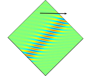
Figure 2. Direct numerical simulation of a sustained turbulent stripe in a large domain with  $L_{x^{\prime }}=L_{z^{\prime }}=400$, no tilting (flow from bottom to top). Isocontours of wall-normal velocity $v(x,y=0,z)$ for $Re=660$. The oblique red rectangle illustrates the concept of tilted domain (Barkley & Tuckerman Reference Barkley and Tuckerman2005) with periodic boundary conditions in $x$ and $z$. By construction, the shorter side of the domain is parallel to the stripe.
The resolution used for a numerical domain with  $(L_{x},L_{z})=(10,40)$ is $N_{x}=72$, $N_{y}=49$ and $N_{z}=256$ for all values of $Re$ and $\unicode[STIX]{x1D703}$ reported. This is comparable with the resolution in Tuckerman et al. (Reference Tuckerman, Kreilos, Schrobsdorff, Schneider and Gibson2014) for the turbulent regimes, known to be computationally more demanding in terms of resolution than edge regimes for equivalent parameters. One can also define a local resolution ( $n_{x}=N_{x}/L_{x}$, $n_{z}=N_{z}/L_{z}$) maintained in case of changes in domain size (such as in § 3.1). The current value of $N_{y}$ ensures that, for values of $Re$ sufficiently below 1000, all transverse scales are properly resolved.
In what follows, we keep primed notations ( $x^{\prime },z^{\prime },u^{\prime },w^{\prime }$) for non-tilted planar variables and non-primed notations ( $x,z,u,w$) for planar quantities defined within a tilted domain. The physical streamwise velocity perturbation is hence denoted $u^{\prime }$ (respectively, $w^{\prime }$ for the spanwise component), while the velocity components parallel and orthogonal to the stripes are denoted $u$ and $w$, respectively.
2.1 Tools for identification of nonlinear solutions
The observable  $E_{v}$, based on the deviation from the base flow, is the wall-normal energy defined as
 $$\begin{eqnarray}E_{v}=\frac{1}{2}\int _{0}^{L_{x}}\int _{0}^{L_{z}}\int _{-1}^{1}v^{2}\,\text{d}x\,\text{d}y\,\text{d}z,\end{eqnarray}$$
 where  $v$ is the wall-normal velocity component. The total perturbation kinetic energy $E$ is defined in a similar way with $v^{2}$ replaced by the squared norm of the disturbance velocity $|\boldsymbol{u}|^{2}$ (both independent of the tilting of the domain). The $z$-dependent energy $e(z)$ is defined by
 $$\begin{eqnarray}e(z)=\frac{1}{2}\int _{0}^{L_{x}}\int _{-1}^{1}|\boldsymbol{u}|^{2}\,\text{d}y\,\text{d}x,\end{eqnarray}$$
 and is such that  $E=\int _{0}^{L_{z}}e(z)\,\text{d}z$. Its wall-normal counterpart $e_{v}(z)$ is also defined in the same manner by considering only $v^{2}$ as integrand.
Edge states are computed using the standard bisection algorithm (Skufca, Yorke & Eckhardt Reference Skufca, Yorke and Eckhardt2006; Schneider, Eckhardt & Yorke Reference Schneider, Eckhardt and Yorke2007; Duguet, Schlatter & Henningson Reference Duguet, Schlatter and Henningson2009): the amplitude of an arbitrary initial condition is rescaled recursively until the flow reaches neither laminar nor turbulent level for sufficiently long observation times. The two criteria, according to which trajectories are labelled as relaminarising or transitioning, are based on threshold values for the wall-normal energy  $E_{v}$ (see (2.5)), both chosen after trial and error. Once machine precision is reached, the rescaling process is re-started from a state at a later time.
Several types of exact coherent states are identified during this study. In particular, TW solutions are defined by
 $$\begin{eqnarray}\boldsymbol{u}(x,y,z,t)=\boldsymbol{u}(x+c_{x}T,y,z+c_{z}T,t+T),\end{eqnarray}$$
 for all  $t$ and $T$, where $t$ is time and $T$ is time period, while relative periodic orbits (RPOs) are defined as
 $$\begin{eqnarray}\boldsymbol{u}(x,y,z,t)=\boldsymbol{u}(x+\unicode[STIX]{x1D70E}_{x},y,z+\unicode[STIX]{x1D70E}_{z},t+T),\end{eqnarray}$$
 for all  $t$ but for given values of $T$,
$T$,  $\unicode[STIX]{x1D70E}_{x}$ and $\unicode[STIX]{x1D70E}_{z}$, where $\unicode[STIX]{x1D70E}_{x}$ and $\unicode[STIX]{x1D70E}_{z}$ are shifts in the $x$ and $z$ directions respectively. The Newton–Krylov algorithm included in channelflow.org, augmented by the hook–step globalisation technique (Viswanath Reference Viswanath2007), is used to successfully converge TW solutions and RPOs with an accuracy of $O(10^{-14})$. Arclength continuation is used to track the converged states as functions of various parameters, such as $Re$,
$Re$,  $L_{x}$ or $\unicode[STIX]{x1D703}$. For each converged state, application of the matrix-free Arnoldi algorithm is used to determine eigenvalues or Floquet exponents of converged solutions.
The governing system of equations, independent of the numerical domain, is equivariant with respect to the two discrete symmetries
 $$\begin{eqnarray}\displaystyle & \displaystyle S_{y}:[u^{\prime },v,w^{\prime }](x^{\prime },y,z^{\prime })\rightarrow [u^{\prime },-v,w^{\prime }](x^{\prime },-y,z^{\prime }), & \displaystyle\end{eqnarray}$$
 $$\begin{eqnarray}\displaystyle & \displaystyle S_{z}^{\prime }:[u^{\prime },v,w^{\prime }](x^{\prime },y,z^{\prime })\rightarrow [u^{\prime },v,-w^{\prime }](x^{\prime },y,-z^{\prime }). & \displaystyle\end{eqnarray}$$
 This implies that for any solution  $\boldsymbol{u}^{\prime }(\boldsymbol{x}^{\prime })$, $(S_{y}\boldsymbol{u}^{\prime })(\boldsymbol{x}^{\prime })$ and $(S_{z}^{\prime }\boldsymbol{u}^{\prime })(\boldsymbol{x}^{\prime })$ are also solutions. In particular, any oblique stripe forming an angle $\unicode[STIX]{x1D703}$ with the streamwise direction is associated with its symmetric counterpart, an oblique stripe with an angle $-\unicode[STIX]{x1D703}$. This degeneracy is eliminated when computing in a tilted domain with $\unicode[STIX]{x1D703}\neq 0^{\circ }$ and $\unicode[STIX]{x1D703}\neq 90^{\circ }$, yet it is useful to keep in mind that all the solutions listed come in pairs.
Another symmetry (linked to the tilted geometry) is the shift-and-reflect symmetry with shifts in the  $x$-direction.
 $$\begin{eqnarray}S_{rx}:[u,v,w]\left(x+\frac{L_{x}}{2},y,z\right)\rightarrow [u,-v,w](x,-y,z).\end{eqnarray}$$
 This symmetry, specific to each value of  $L_{x}$, has not been imposed in any of the computations, but it turns out to be verified by all TW solutions found.
3 Parametric study
3.1 Edge tracking
The first attempt to identify a simple edge state dynamics is for  $Re=720$, $\unicode[STIX]{x1D703}=35^{\circ }$, $L_{x}=10$ and $L_{z}=40$. These values of $L_{x}$ and $L_{z}$ are similar to those in Tuckerman et al. (Reference Tuckerman, Kreilos, Schrobsdorff, Schneider and Gibson2014), whereas $\unicode[STIX]{x1D703}=35^{\circ }$ is well within the experimental and numerical range. The initial condition consists of a random three-dimensional divergence-free velocity field. As shown in figure 3(a), the energy $E(t)$ settles to a constant value, the signature of a TW – which can be converged easily using the Newton–Krylov algorithm (Duguet, Willis & Kerswell Reference Duguet, Willis and Kerswell2008). The solution travels with a phase velocity $\boldsymbol{c}$ with non-zero streamwise and spanwise components $c_{x^{\prime }}=0.77=1.15U_{b}$ and $c_{z^{\prime }}=0.06$ in units of $U_{cl}$, where $U_{b}=2/3\ast U_{cl}$ is a bulk velocity. The TW propagates with a streamwise phase velocity slightly larger than the flow rate: fluid enters the wave from upstream and is released downstream of it as well as on the sides. The property that lower-branch solutions travel faster than the base flow appears generic to all wall-bounded shear flows. By virtue of the $S_{z}$ symmetry, a twin TW solution also exists in a domain tilted with angle $-\unicode[STIX]{x1D703}$ with opposite spanwise propagation velocity.
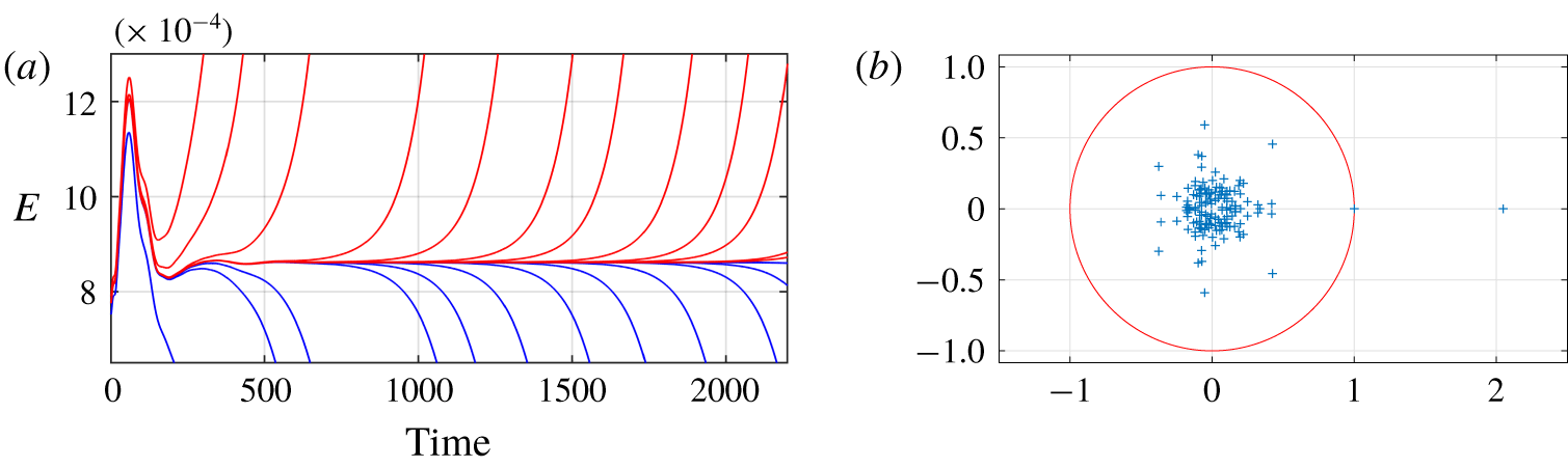
Figure 3. (a) Edge tracking in a domain tilted by  $\unicode[STIX]{x1D703}=35^{\circ }$ at $Re=720$. Trajectories in blue relaminarise directly whereas trajectories in red become turbulent. (b) Eigenspectrum for the converged lower-branch TW (LBTW) solution with $\unicode[STIX]{x1D703}=35^{\circ }$, $Re=720$, $L_{x}=3.33$ and $L_{z}=40$, computed using the Arnoldi algorithm with time horizon $T=60$. Only one multiplier lies outside the unit circle.
The initial bisections were carried out for  $L_{x}=10$. The numerical domain with these parameters accommodates three identical wavelengths, and the TWs found do possess this 3-fold periodicity in $x$. This suggests that a similar TW solution should exist as an edge state in a numerical domain with $L_{x}\leftarrow L_{x}/3$ and correspondingly $N_{x}\leftarrow N_{x}/3$. This is indeed the case for $L_{x}=3.33$. From here on, unless otherwise stated, the value of $L_{x}$ is set to 3.33. The new TW identified possesses the $S_{rx}$ symmetry specific to the new value of $L_{x}$ (compatible with the different symmetry identified for $L_{x}=10$). We do not exclude possible subharmonic instabilities for larger values of $L_{x}$.
It was determined using the Arnoldi algorithm that the TW solution is linearly unstable but possesses only one real unstable eigenvalue, as expected for edge states. This corresponds to one unstable Floquet multiplier outside the unit circle in figure 3(b). The same property also holds for  $L_{x}=6.66$, 10 and 13.33.
3.2 Spatial localisation
Similar bisections were repeated for different values of  $L_{z}=20$, 40, 80 and 120. The numerical resolution was kept identical except in the $z$-direction in which $N_{z}$ was kept proportional to $L_{z}$. In all cases, a similar-looking TW solution was identified as an edge state and converged successfully using the Newton algorithm. The $z$-dependence of the perturbation kinetic energy of the four TWs obtained for different $L_{z}$ is shown in figure 4. All TWs found here are spatially localised. This suggests that the corresponding TW for $L_{z}\rightarrow \infty$ is a solitary state (its energy drops off exponentially). In what follows, the value of $L_{z}$ is fixed to 40, keeping in mind that most results are independent of $L_{z}$ provided $L_{z}$ is large enough.
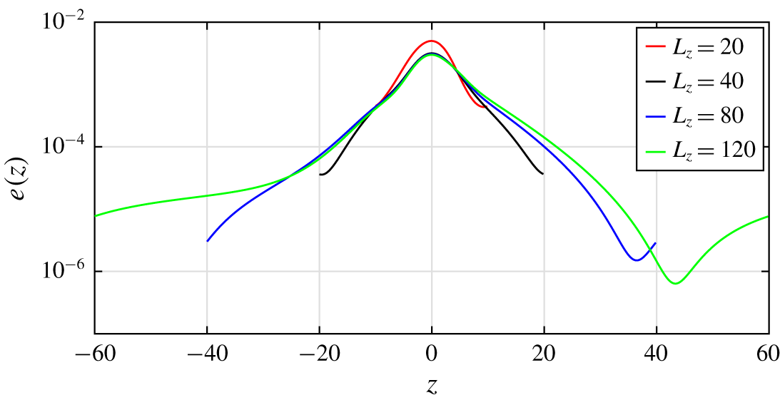
Figure 4. Perturbation kinetic energy  $e(z)$ for LBTWs with increasing $L_{z}=20$, 40, 80 and 120 (logscale). $L_{x}=3.33$, $\unicode[STIX]{x1D703}=35^{\circ }$, $Re=720$.
3.3 Self-sustenance and large-scale flow
We now display visualisations of the TW solutions for 45 $^{\circ }$ in figures 5 and 6. The $xz$-view of the wall-normal velocity in the midplane (see figure 5) reveals a spatial structure very similar to that of turbulent stripes. The three-dimensional structure (see figure 6) features streamwise vortices which are almost parallel to the streamwise direction. Streamwise vortices are naturally associated with streaks (spanwise modulations of the streamwise velocity). The tails of the streaks outside the core of the stripe are deviated by the large-scale flow near both interfaces (Henningson & Kim Reference Henningson and Kim1991; Duguet & Schlatter Reference Duguet and Schlatter2013). Interestingly, the streaks for the LBTWs shown in figure 6(a,b), do not feature the characteristic sinuous structure of other exact coherent states found in smaller domains and fundamental to Waleffe’s self-sustaining process (Waleffe Reference Waleffe1998). This process assumes that the streamwise vorticity induced by sinuous streak instabilities compensates for its own viscous decay, and that this loop maintains the exact coherent structures in equilibrium. Here, the streamwise rolls are not sinuous; however, their slight deviation by the large-scale flow contributes to their three-dimensionalisation. This suggests that the nonlinear feedback on the streamwise vorticity, necessary for its sustenance against viscous decay, is operated by the tilting due to the large-scale flow, rather than by the sinuous instability of the streaks. Further work would be necessary to confirm this mechanism. Unlike the LBTW solutions, the UBTW solutions do feature sinuous oscillations of the streaks visible in figure 6(c,d).
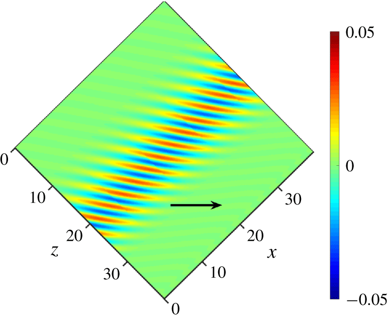
Figure 5. LBTW solution computed in a domain tilted by  $\unicode[STIX]{x1D703}=45^{\circ }$ for $Re=720$, $L_{x}=3.33$ and $L_{z}=40$ represented using 12 concatenated copies. Wall-normal velocity field $v(x,y=0,z)$ (streamwise direction pointing towards positive $x$ and $z$).
$z$).
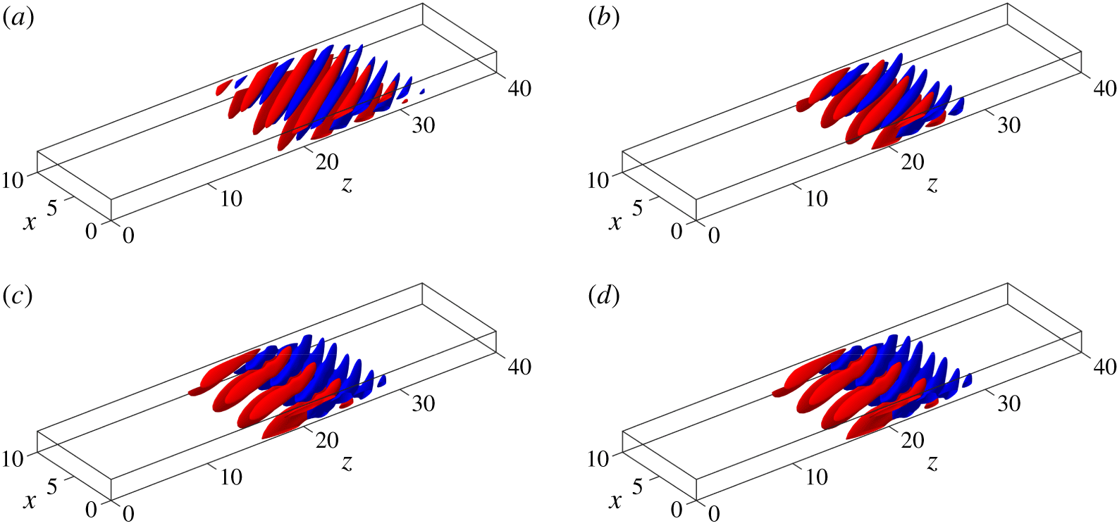
Figure 6. (a) LBTW solution at  $Re=720$. (b) LBTW solution at $Re=414.25$. (c) Upper-branch TW (UBTW) solution at $Re=414.25$. (d) UBTW solution at $Re=438.74$. Isolevels of streamwise velocity perturbation (red: $u_{x}=0.1$, blue: $u_{x}=-0.1$) for (a–d). (a–d) Three concatenated copies only.
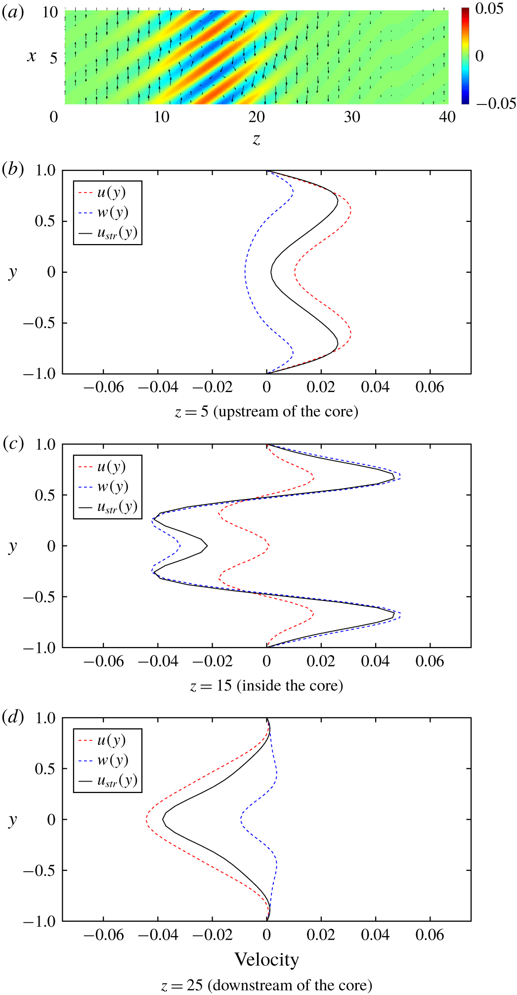
Figure 7. Velocity field of LBTW solution at  $Re=720$ at $\unicode[STIX]{x1D703}=45^{\circ }$. (a) The $xz$-plane with $y$-averaged velocity components as quivers and wall-normal velocity using contours (streamwise direction pointing towards positive $x$ and $z$). (b–d) The $x$-averaged velocity profiles as functions of $y$ for $z=5,15$ and 25. These profiles show the large-scale flow around the stripe.
We investigate now the spatial structure of this large-scale flow. In figure 7(a), the planar velocity components are plotted after integration in  $y$ from wall to wall. As predicted in Duguet & Schlatter (Reference Duguet and Schlatter2013), this $y$-integrated velocity field is parallel to the interface of the stripe. This observation is fully consistent with the mean flow properties (Barkley & Tuckerman Reference Barkley and Tuckerman2007) and with instantaneous visualisations of turbulent stripes (Xiong et al. Reference Xiong, Tao, Chen and Brandt2015). The simple time-dependence of the TW solution makes the structure of the integrated large-scale flow emerge even without spatial filtering or time-averaging. The non-integrated flow has a strongly three-dimensional structure lost by averaging. The individual components of large-scale flow and their dependence on $y$ are plotted in figure 7(b–d), after averaging in the short stripe direction $x$, and at different $z$ positions outside and inside the active part of the stripe. Robust conclusions emerge independently of the value (positive or negative) of the angle $\unicode[STIX]{x1D703}$. In all cases, the large-scale flow upstream of the stripe has a parallel component pointing downstream, whereas the large-scale flow downstream of the stripe has a parallel component pointing upstream. The large-scale flow outside the active zone differs depending on the side of the stripe considered: the velocity profile upstream is double-humped and stronger near the walls, whereas the velocity profile downstream is single-humped and stronger near the midgap. None of the local velocities exceeds 0.04 (in units of $U_{cl}$) in absolute value, and such values are attained in the active part of the stripe (here at $z=15$).
3.4 Angular dependence
The same strategy as in § 3.1 was repeated for all values of  $\unicode[STIX]{x1D703}$ between 0 and 90 $^{\circ }$ in steps of 5 $^{\circ }$, by fixing $L_{x}=3.33$ and $L_{z}=40$. The original value of $Re$ was chosen again as 720, high enough for turbulent stripes to be observable in numerical simulations. As observed in Barkley & Tuckerman (Reference Barkley and Tuckerman2007) and Duguet et al. (Reference Duguet, Schlatter and Henningson2010), not all angles can support a stable laminar–turbulent interface. Bisection was successful at converging TWs as edge states only for 25 $^{\circ }\leqslant \unicode[STIX]{x1D703}\leqslant$ 60 $^{\circ }$. Outside this range, edge tracking proved unfeasible because the turbulent state itself was only short-lived. Continuation of the TWs in $Re$ was performed at fixed values of $\unicode[STIX]{x1D703}$, $L_{x}$ and $L_{z}$ for the values of $\unicode[STIX]{x1D703}$ where TWs were found for $Re=720$. For each angle, the corresponding TWs emerge in a saddle-node bifurcation at a given value of $Re=Re_{SN}(\unicode[STIX]{x1D703},L_{x},L_{z})$ (where $Re_{SN}$ is $Re$ at saddle node bifurcation). This is shown in figure 8, where the total kinetic energy $E$ is plotted against $Re$ for several angles. This figure also contains information on the linear stability of the waves (analysed later). Continuation along the upper branch was stopped as soon as resolution issues started to manifest themselves, a commonly reported issue for upper-branch solutions of shear flows (Waleffe Reference Waleffe2001). The smallest value of $Re_{SN}$ is apparently obtained for $\unicode[STIX]{x1D703}=45^{\circ }$. Figure 9 displays similar curves for the streamwise and spanwise phase velocities, plotted versus $Re$. Here, the LBTWs are characterised by the larger phase velocities. All TW solutions were found to obey the $S_{rx}$ symmetry for all imposed angles.
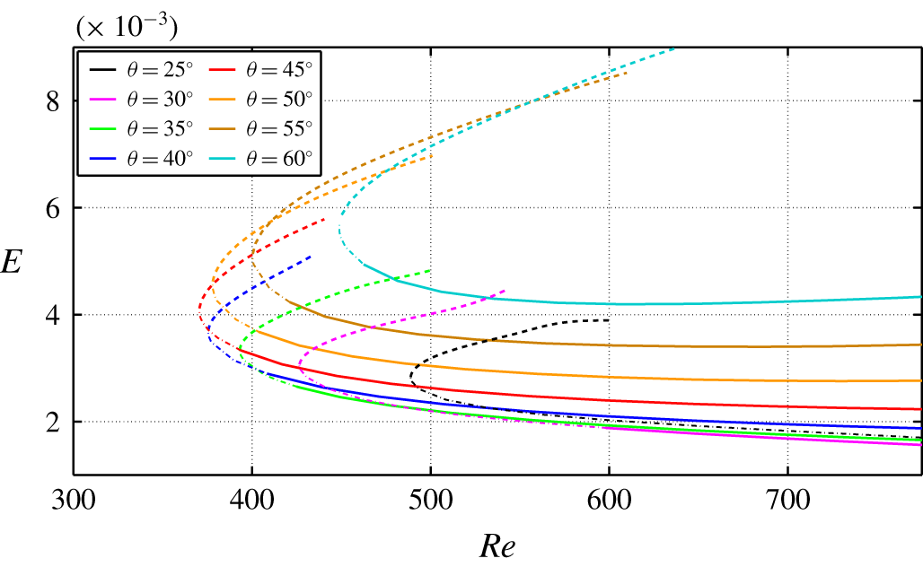
Figure 8. Energy for TW solutions versus  $Re$ in a domain for different angles $\unicode[STIX]{x1D703}$, $L_{x}=3.33$ and $L_{z}=40$. Solid lines: TWs with one unstable eigenvalue only (edge states); thin dotted lines: LBTWs with strictly more than one unstable eigenvalue; thick dotted lines: UBTWs.
Continuation is next carried out in the angle parameter  $\unicode[STIX]{x1D703}$ for fixed $Re$. This turns out to be a more efficient way to explore the limits of the range of angles where TWs are found. Such data are shown in figure 10 in a effort to highlight the three-dimensional structure of the diagram shown in figures 8 and 9. As shown in figure 10, the range of angles shrinks to the sole value of $45^{\circ }$, whereas it monotonically widens for increasing $Re$. For $Re=720$, the largest value of $Re$ explored in this study, possible angles range from $20^{\circ }$ to almost $70^{\circ }$, slightly wider than the range of values of $\unicode[STIX]{x1D703}$ accessible by bisection at the same $Re$. It is instructive to plot the value of $Re_{SN}(\unicode[STIX]{x1D703})$ versus $\unicode[STIX]{x1D703}$ for fixed $L_{x}$ and $L_{z}$ (cf. figure 12). The curve appears as a slightly asymmetric parabola centred around $45^{\circ }$. This curve bounds the region of existence of the TW solutions in parameter space. As $Re$ is gradually increased from zero, the first TW encountered has $\unicode[STIX]{x1D703}=45^{\circ }$. As $Re$ continues to increase, the range of possible angles widens.
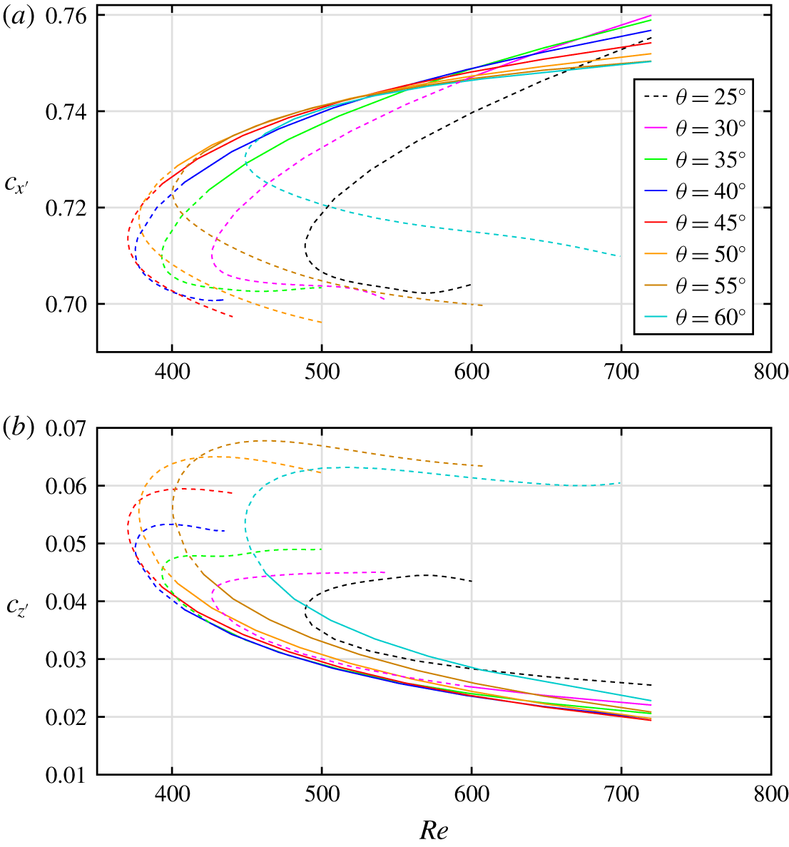
Figure 9. Phase velocities for TW solutions in a domain tilted by  $\unicode[STIX]{x1D703}$ with $L_{x}=3.33$ and $L_{z}=40$. (a) Streamwise component, $c_{x^{\prime }}(Re)$. (b) Spanwise component $c_{z^{\prime }}(Re)$.
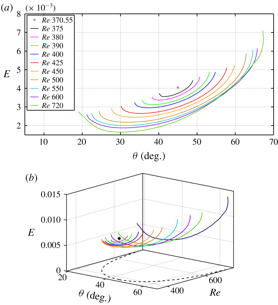
Figure 10. Continuation of the TWs in angle for different values of  $Re$. (a) The $(\unicode[STIX]{x1D703},E)$ projection. (b) Three-dimensional projection $(\unicode[STIX]{x1D703},Re,E)$.
The width of the localised stripe along  $z$ can be evaluated by choosing an arbitrary criterion $e_{v}(z)\geqslant 10^{-4}$. It corresponds to the length of the streaks as visualised in figure 5. The width across the streamwise direction, i.e. along $x^{\prime }$, was determined from the previous criterion using trigonometric rules. As suggested in figure 4, these quantities are independent of the value of the parameter $L_{z}$ once it is large enough. For a constant value of $Re$, the width increases almost linearly with $\unicode[STIX]{x1D703}$, see figure 11. The maximum amplitude of these waves, however, is lowest around $45^{\circ }$ as is shown in figure 11 using $z$-profiles of $e_{v}$. No clear reason for this property has been identified yet.
Figure 11. (a) Profile of  $e_{v}(z)$ for various tilt angles, $L_{x}=3.33$, $L_{x}=40$, $Re=720$, lower-branch solutions. (b) Stripe width versus $\unicode[STIX]{x1D703}$ for $Re=720$, both along the streamwise direction (blue) and across the stripe (red).
3.5 Hopf bifurcations
As can be seen in figure 8, the stability of each TW family parametrised by  $\unicode[STIX]{x1D703}$ changes with $Re$ along its respective lower branch. A similar scenario emerges for all values of $\unicode[STIX]{x1D703}$. As $Re$ is decreased, starting from $Re=720$, the LBTW initially possesses one unstable eigenvalue only and is an edge state of the corresponding system. At a given value of $Re=Re_{H}(\unicode[STIX]{x1D703},L_{x},L_{z})$ (where $Re_{H}$ is $Re$ at Hopf bifurcation), two additional complex conjugate eigenvalues become unstable, so that between $Re_{H}$ and $Re_{SN}<Re_{H}$ the TW is no longer an edge state.
For each set of parameters, a Hopf bifurcation at  $Re=Re_{H}$ leads to a new branch of RPOs of period $T$, initially unstable close to $Re_{H}$. The loci of these Hopf bifurcation points are shown in figure 12 together with the saddle-node points. In fact, other bifurcations of TWs occur in the interval $(Re_{SN},Re_{H})$, as is clear from the number of unstable eigenvalues at $Re_{SN}$ listed in table 1, which always exceeds three. For instance, for $\unicode[STIX]{x1D703}=45^{\circ }$, $L_{x}=3.33$ and $L_{z}=40$, the primary Hopf bifurcation (for descending $Re$) occurs at $Re_{H}\approx$ 393, while the saddle-node bifurcation lies at $Re_{SN}=370.55$. This Hopf bifurcation breaks the $S_{rx}$ symmetry. The resulting branch of RPOs has been tracked by continuation. One snapshot is displayed in figure 13 using three concatenated copies. Another Hopf bifurcation arises near $Re=390$. We have not investigated the possible additional bifurcations along the upper branch and/or for other angles and domain sizes. The Hopf bifurcation points ( $\unicode[STIX]{x1D703}$, $Re_{H}(\unicode[STIX]{x1D703})$) get increasingly far from the saddle-node points as $\unicode[STIX]{x1D703}$ decreases. The values for the period of the RPOs at their respective bifurcation points are reported for most angles in tables 1 and 2.
Unlike the LBTW solutions, the RPO features sinuous oscillations of the streaks. In a frame moving with the original TW velocity, the RPO displays global time-periodic oscillations visible only in the core of the corresponding TW. In this moving frame, they travel upstream, as attested by the space–time diagram in figure 14. The emergence of finite-amplitude time-periodic oscillations propagating on top of a spatially localised TW is strongly reminiscent of the concept of nonlinear global mode put forward in spatially inhomogeneous media (Pier & Huerre Reference Pier and Huerre1996). In this picture, the period of the global oscillations is determined at the location where local stability analysis predicts transition from convective to absolute instability. The role of the slowly spatially evolving base flow is played here by the localised TW solutions, for which local stability analysis is known to predict absolute instability in the core but stability in the more laminar zones.
Figure 12. Location of saddle-node bifurcations in a  $(\unicode[STIX]{x1D703},Re)$ representation ( $Re_{SN}(\unicode[STIX]{x1D703})$, blue solid line), and Hopf bifurcation points ( $Re_{H}(\unicode[STIX]{x1D703})$, red dots) below which the TWs are no longer edge states.
Table 1. Values of  $Re$ at the saddle-node bifurcation point $Re_{SN}$ and at the Hopf bifurcation point $Re_{H}$ of TW solutions for different tilt angles $\unicode[STIX]{x1D703}$ and for $L_{x}=3.33$ and $L_{z}=40$. For $Re>Re_{H}$ the LBTWs are edge states. Also listed is the stability at the saddle-node point with number of unstable eigenvalues and also the Hopf bifurcation point for LBTW solution branches. See text for definitions.
Figure 13. Snapshot of an RPO solution computed in a domain tilted by  $\unicode[STIX]{x1D703}=45^{\circ }$ for $Re=407$, $L_{x}=3.33$ and $L_{z}=40$, three concatenated copies. Isolevels of streamwise velocity perturbation (red $u_{x}=+0.13$, blue: $u_{x}=-0.13$) and streamwise vorticity (yellow: $\unicode[STIX]{x1D714}_{x}=1.0$, green: $\unicode[STIX]{x1D714}_{x}=-1.0$).
Table 2. Time period  ${T_{p}}_{1}$ (respectively ${T_{p}}_{2}$) of the first (respectively second, if any) RPO bifurcating from the LBTW branch for various tilt angles (deduced from the eigenvalues at their respective Hopf bifurcation). The period ${T_{p}}_{1}$ is computed at $Re=Re_{H}$.
Figure 14. Space–time diagram  $e_{v}(z,t)$ for the RPO solution shown in figure 13 over three time periods, $Re=407$. Frame moving with the original LBTW phase velocity computed for the same value of $Re$.
$Re$.
3.6 Minimum Reynolds number
A recurrent interrogation in earlier investigations of invariant solutions is the minimal value of  $Re$ supporting such equilibrium solutions. For instance, Wall & Nagata (Reference Wall and Nagata2016) have lately reported a non-tilted TW solution existing down to $Re=665$. This minimisation task can appear endless here given the many parameters present. However, we shortcut this limitation by recalling that (i) the new TW solutions become independent of $L_{z}$ for $L_{z}$ large enough, and (ii) the minimal $Re$ corresponds to $\unicode[STIX]{x1D703}=45^{\circ }$. As a consequence, we define here, pragmatically, the globally minimal Reynolds number as $Re_{m}=\min _{L_{x}}Re_{SN}(\unicode[STIX]{x1D703}=45^{\circ },L_{x},L_{z}=40)$. Hence, $Re_{m}$ can be determined by fixing $\unicode[STIX]{x1D703}=45^{\circ }$, $L_{z}=40$ and performing continuation in $Re$ for several values of $L_{x}$ only. In figure 15, $Re_{m}$ is displayed as a function of $L_{x}$. A local minimum for $Re_{m}$ is found around 367 and occurs for $L_{x}=3.2$. Note that this value is close to the value of 3.33 used here. We do not exclude the possibility for other local minima corresponding to other yet unreported families of TW solutions.
Figure 15. Minimum  $Re$ versus $L_{x}$ for $\unicode[STIX]{x1D703}=45^{\circ }$ and $L_{z}=40$.
4 Discussions and outlook
We have presented new families of nonlinear TW solutions of channel flow featuring spatial localisation, oblique orientation with respect to the mean flow direction, streamwise vortices and streaks. All the solutions reported here are linearly unstable, although the number of unstable directions is generally very low, ranging from one for edge states up to six for upper-branch solutions near their onset. These solutions are the ones appearing at the lowest value of  $Re$ reported so far in channel flow. Interestingly, they do not emerge via a homoclinic snaking scenario as is the case for many non-tilted localised states (Schneider, Gibson & Burke Reference Schneider, Gibson and Burke2010; Knobloch Reference Knobloch2015). A few Hopf bifurcations of these new waves occur along the lower branch, rather than the upper branch as commonly reported in shear flows (as in e.g. Zammert & Eckhardt (Reference Zammert and Eckhardt2015)). The occurrence of such Hopf bifurcations means that for $Re_{SN}<Re<Re_{H}$ the TWs are no longer edge states and cannot be identified using edge tracking. The success of the method used here hence relies on starting at a sufficiently high value of $Re$.
$Re$.
This dynamical systems approach to complex stripe patterns can also be applied to other systems displaying spatiotemporal intermittency. The application of edge tracking in tilted domains of plane Couette flow has so far yielded only chaotic edge states rather than exact solutions, even with central symmetry imposed. While this highlights some limitations of the current method, other ways of constructing exact localised solutions are possible, as shown in Gibson & Brand (Reference Gibson and Brand2014) for plane Poiseuille flow using spatial windowing or using asymptotic analysis (Deguchi & Hall Reference Deguchi and Hall2015) in plane Couette flow. We also note a recent cheaper alternative to edge tracking using feedback control (Willis et al. Reference Willis, Duguet, Omel’chenko and Wolfrum2017) likely to work successfully in our case. More recently, similar families of oblique localised solutions of plane Couette flow have also been constructed by exploiting the possible subharmonic instabilities of formerly known non-localised states (Reetz, Kreilos & Schneider Reference Reetz, Kreilos and Schneider2019; Reetz & Schneider Reference Reetz and Schneider2020). This is another promising alternative to edge tracking, although it requires good preliminary knowledge of some solutions. An extension of these ideas to other geometries is encouraged.
For the last two decades, the main motivation to detect and study unstable nonlinear states comes from the conjecture that they constitute a state-space skeleton for the turbulent dynamics (Hof et al. Reference Hof, van Doorne, Westerweel, Nieuwstadt, Faisst, Eckhardt, Wedin, Kerswell and Waleffe2004; Eckhardt et al. Reference Eckhardt, Schneider, Hof and Westerweel2007; Kawahara et al. Reference Kawahara, Uhlmann and Van Veen2012). TW states, like those reported here, are the simplest instances of such states compatible with the symmetries of the system. The different Hopf bifurcations of these waves lead to new branches of unstable periodic orbits whose further bifurcations, both local and global, are expected to cover the turbulent attractor specific to each tilted domain (Avila et al. Reference Avila, Mellibovsky, Roland and Hof2013; Zammert & Eckhardt Reference Zammert and Eckhardt2015). This approach is now generally accepted for small constrained systems Budanur et al. (Reference Budanur, Short, Farazmand, Willis and Cvitanović2017). However, it remains daring to extend it to spatiotemporal complex situations, such as turbulent stripes, where additional spatial degrees of freedom come into play. Further bifurcations of these modulated waves are expected to give rise to a regime of temporal chaos, which is dynamically consistent with the turbulent behaviour reported – in both constrained and unconstrained numerical domains – at comparable values of  $Re$ (Tuckerman et al. Reference Tuckerman, Kreilos, Schrobsdorff, Schneider and Gibson2014).
At the lowest  $Re$ typical of figure 1, the experimental transition process involves solitary finite-length bands fully localised in one direction and growing (or receding) in another direction. These bands feature an active head and a passive rear (see e.g. Kanazawa (Reference Kanazawa2018), chap. 5 and Xiao & Song (Reference Xiao and Song2020) or figure 2). While growth occurs at the active head, at slightly larger $Re$, stripes extend to lateral boundaries and do not necessarily have a well-defined head. This suggests that the core of the stripe is autonomous and self-sustained. The solutions presented here are localised only in one direction and have unambiguous similarities with the core of the turbulent stripes.
Such an analogy between TWs and turbulence is supported by the agreement between the spanwise wavelength and the streamwise extent of the streaks. More originally, a large-scale flow parallel to the band direction is common to both turbulent stripes and the present TWs. It has been suggested as a crucial player for the spatial proliferation of turbulence in planar flows and as a mechanism to justify the obliqueness of the laminar–turbulent interfaces (Duguet & Schlatter (Reference Duguet and Schlatter2013)). This large-scale flow property is specific to localised turbulence. It cannot be interpreted theoretically using the previously found non-localised states, and this justifies the present search for oblique solutions localised in one direction only. A posteriori, we have verified that the large-scale flow induces a spanwise propagation velocity explaining the motion of the streaks within the band itself (cf. figure 9). From the investigation of the exact solutions, it was also suggested that the large-scale flow plays a role in the regeneration of the streamwise vorticity inside the band core. Such a possibility had not been considered so far for localised turbulent dynamics, which highlights the utility of exact solutions. As far as the understanding of the energy production mechanisms at the head is concerned, however, other channel solutions with an additional direction of localisation need to be envisioned (Zammert & Eckhardt Reference Zammert and Eckhardt2014; Kanazawa Reference Kanazawa2018).
At slightly higher  $Re$, the multitude of possible angles displayed by turbulent stripe patterns falls within the range of angle values where the TWs and their bifurcated states exist. A natural question that arises is whether the range of angles of the TWs bears a direct relation to the selection process of stripe angles in turbulent flows. The critical curve $\unicode[STIX]{x1D703}(Re)$ displayed in figure 12 is at first sight reminiscent of the selection mechanism in other systems with one spatial degree of freedom, such as Rayleigh–Bénard convection (Cross & Hohenberg Reference Cross and Hohenberg1993). However, the nonlinear nature of the wave solutions makes the selection mechanism entirely different. As a consequence of nonlinearity, adding different such solutions together to create new solutions is not allowed. A consequence is that different routes to chaos for different values of $\unicode[STIX]{x1D703}$ coexist. On the other hand, the TW with $45^{\circ }$ is the one persisting down to the lowest $Re$. This is reminiscent of the observation that, close to their onset in $Re$ where they are observed, the angle of turbulent stripes saturates at $45^{\circ }$ (Tao et al. Reference Tao, Eckhardt and Xiong2018; Paranjape Reference Paranjape2019). It remains to be understood why no turbulent stripe forms or sustains with an angle larger than $45^{\circ }$ in realistic domains, whereas this is allowed for TW solutions. This apparent discrepancy is likely to be related to the choice of the tilted domains rather than to the TWs themselves. Indeed, in the comparable tilted domains of plane Couette flow, turbulence is also reported for angles higher than $45^{\circ }$ (Barkley & Tuckerman Reference Barkley and Tuckerman2007), whereas it is not the case in large periodic domains (Duguet et al. Reference Duguet, Schlatter and Henningson2010). This might be related to the issue of stability (in the broad sense) of a given laminar–turbulent interface.
Acknowledgements
The authors thank S. Zammert and B. Budanur for useful discussions. J. F. Gibson is gratefully acknowledged for the development and the maintenance of the code Channelflow. Y.D. would like to thank P. Schlatter and D. S. Henningson for an early collaboration on a similar topic in the case of plane Couette flow during the years 2008–2013.
Declaration of interests
The authors report no conflict of interest.


 Open access