


1 Introduction
Two-dimensional (2-D) and quasi-2-D flows occur at the macro- and mesoscale in a variety of physical systems. Examples include plasma flow in the solar tachocline (Spiegel & Zahn Reference Spiegel and Zahn1992), Earth’s atmosphere near the tropopause (Nastrom, Gage & Jasperson Reference Nastrom, Gage and Jasperson1984; Gage & Nastrom Reference Gage and Nastrom1986; Falkovich Reference Falkovich1992), stratified layers in the oceans (Vallis Reference Vallis2006), laboratory experiments using electrolyte layers (Sommeria Reference Sommeria1986) and soap films (Vorobieff, Rivera & Ecke Reference Vorobieff, Rivera and Ecke1999) and, more recently, also dense bacterial suspensions, where the collective motion of microswimmers induces patterns of mesoscale vortices (Dombrowski et al. Reference Dombrowski, Cisneros, Chatkaew, Goldstein and Kessler2004; Dunkel et al. Reference Dunkel, Heidenreich, Drescher, Wensink, Bär and Goldstein2013; Gachelin et al. Reference Gachelin, Rousselet, Lindner and Clement2014). A characteristic feature of 2-D turbulence is the occurrence of an inverse energy cascade (Kraichnan Reference Kraichnan1967), whereby kinetic energy is transferred from small to large scales. Kraichnan’s theoretical prediction has been verified in experimental studies of thin fluid layers (Sommeria Reference Sommeria1986; Paret & Tabeling Reference Paret and Tabeling1997, Reference Paret and Tabeling1998) and through numerical simulations (Lilly Reference Lilly1969; Frisch & Sulem Reference Frisch and Sulem1984; Verron & Sommeria Reference Verron and Sommeria1987), to name only the first few. A detailed overview on 2-D turbulence can be found in the review article by Boffetta & Ecke (Reference Boffetta and Ecke2014). In confined systems, this self-organisation can result in the formation of large-scale coherent structures (Kraichnan Reference Kraichnan1967; Hossain, Matthaeus & Montgomery Reference Hossain, Matthaeus and Montgomery1983; Sommeria Reference Sommeria1986; Smith & Yakhot Reference Smith and Yakhot1993), so-called condensates (Smith & Yakhot Reference Smith and Yakhot1993). These may emerge in different forms depending on the geometry and boundary conditions, e.g. as vortex monopoles in the case of experimental conditions, i.e. wall-bounded flows (Sommeria Reference Sommeria1986; Paret & Tabeling Reference Paret and Tabeling1998; Molenaar, Clercx & van Heijst Reference Molenaar, Clercx and van Heijst2004; van Heijst, Clercx & Molenaar Reference van Heijst, Clercx and Molenaar2006), if the Rayleigh damping, that is the friction between the moving fluid and the bottom plate of the confining experimental apparatus, is small, or as vortex dipoles or jets (Smith & Yakhot Reference Smith and Yakhot1993; Bouchet & Simonnet Reference Bouchet and Simonnet2009; Frishman, Laurie & Falkovich Reference Frishman, Laurie and Falkovich2017) in the case of periodic boundary conditions.
The inverse energy cascade in 2-D turbulence is connected with an additional inviscid conservation law, that of enstrophy. Physically, it is a consequence of the anisotropic stretching of small-scale vortices by large-scale strain followed by an alignment of the small-scale velocity field around the stretched vortex with the large-scale strain field, thereby reinforcing the latter (Chen et al. Reference Chen, Ecke, Eyink, Rivera, Wan and Xiao2006). However, inverse cascades and thus condensates are not specific to 2-D phenomena. They occur whenever fluctuations in one spatial coordinate are suppressed, as is the case in thin fluid layers (Sommeria & Verron Reference Sommeria and Verron1984; Sommeria Reference Sommeria1986; Paret & Tabeling Reference Paret and Tabeling1997, Reference Paret and Tabeling1998; Shats, Xia & Punzmann Reference Shats, Xia and Punzmann2005; Xia, Shats & Falkovich Reference Xia, Shats and Falkovich2009; Celani, Musacchio & Vincenzi Reference Celani, Musacchio and Vincenzi2010; Xia et al. Reference Xia, Byrne, Falkovich and Shats2011; Musacchio & Boffetta Reference Musacchio and Boffetta2017) or, for instance, in the presence of rapid rotation (Deusebio et al. Reference Deusebio, Boffetta, Lindborg and Musacchio2014; Rubio et al. Reference Rubio, Julien, Knobloch and Weiss2014; Gallet Reference Gallet2015), stratification (Sozza et al. Reference Sozza, Boffetta, Muratore-Ginanneschi and Musacchio2015) or both (Marino et al. Reference Marino, Mininni, Rosenberg and Pouquet2013), and in the presence of a strong uniform magnetic field (Gallet & Doering Reference Gallet and Doering2015) for weakly conducting flows. Another, fully three-dimensional (3-D) mechanism that leads to inverse energy transfer is breaking of mirror symmetry (Waleffe Reference Waleffe1993; Biferale, Musacchio & Toschi Reference Biferale, Musacchio and Toschi2012). In magnetohydrodynamic turbulence, the latter can result in the formation of magnetic condensates through large-scale dynamo action or the inverse cascade of magnetic helicity (Frisch et al. Reference Frisch, Pouquet, Léorat and Mazure1975; Pouquet, Frisch & Léorat Reference Pouquet, Frisch and Léorat1976). Finally, spectral condensation also occurs in toroidal confined plasmas, to the effect that an analogy between 2-D turbulence and toroidal plasma turbulence exists, at least at the level of theoretical models (Horton & Hasegawa Reference Horton and Hasegawa1994) and in phenomenological terms (Shats et al. Reference Shats, Xia and Punzmann2005).
Inverse energy transfer can thus occur in different physical systems, and one could imagine that the onset thereof may depend on the details of the system, such as the dimensionality or the presence of a magnetic field, for instance. Smooth, supercritical and subcritical transitions between non-equilibrium statistically steady states have indeed been observed in this context. In 3-D rotating domains for example, the nature of the transition between forward and inverse energy transfer with respect to the rotation rate depends on the mechanism by which the condensate saturates (Seshasayanan & Alexakis Reference Seshasayanan and Alexakis2018). In the case of weak or vanishing friction with side or bottom walls, the two saturation scenarios are: (i) saturation by viscous effects as in two dimensions, where the condensate becomes sufficiently energetic for the upscale flux to be balanced by viscous dissipation (Chan, Mitra & Brandenburg Reference Chan, Mitra and Brandenburg2012), or (ii) saturation by local cancellation of the rotation rate by the counter-rotating vortex that forms part of the condensate (Alexakis Reference Alexakis2015). In case (i) the transition is supercritical (Seshasayanan & Alexakis Reference Seshasayanan and Alexakis2018), and in (ii) it is subcritical (Alexakis Reference Alexakis2015; Yokoyama & Takaoka Reference Yokoyama and Takaoka2017; Seshasayanan & Alexakis Reference Seshasayanan and Alexakis2018), showing bistability and hysteresis (Yokoyama & Takaoka Reference Yokoyama and Takaoka2017). Similar results have been obtained if the magnitude of the forcing is used as a control parameter at a fixed value of the rotation rate (Yokoyama & Takaoka Reference Yokoyama and Takaoka2017), with random and static forcing both resulting in a subcritical transition. The latter was interpreted as evidence in support of universality. Hysteretic transitions and bistable scenarios also occur in thin layers as a function of the layer thickness (van Kan & Alexakis Reference van Kan and Alexakis2019). Subcriticality in the transition to condensate formation in rapidly rotating Rayleigh–Bénard convection has been connected with non-local energy transfer from the driven scales into the condensate due to persistent phase correlations (Favier, Guervilly & Knobloch Reference Favier, Guervilly and Knobloch2019).
In summary, transitions in cascade directions from direct to inverse and vice versa have received considerable attention in recent years, Alexakis & Biferale (Reference Alexakis and Biferale2018) provide a comprehensive overview thereof. Further to this, certain aspects of condensate dynamics, such as circulation reversals, that occur for weak Rayleigh damping (Sommeria Reference Sommeria1986; Molenaar et al. Reference Molenaar, Clercx and van Heijst2004), and vortex breakdown due to viscous boundary layers (Molenaar et al. Reference Molenaar, Clercx and van Heijst2004), have been investigated experimentally and numerically. Spontaneous transitions between condensates and disordered states have been observed in toroidal plasma turbulence (Shats et al. Reference Shats, Xia and Punzmann2005). However, transitions to purely 2-D turbulence have only been studied in the context of wave turbulence described in terms of the Gross–Pitaevsky equation (Vladimirova, Derevyanko & Falkovich Reference Vladimirova, Derevyanko and Falkovich2012), and in active matter. In the former, the transition depends on the details of the small-scale driving, i.e. it is non-universal. In the latter, spatio-temporal chaos and classical 2-D turbulence with a condensate are connected by a subcritical transition (Linkmann et al. Reference Linkmann, Boffetta, Marchetti and Eckhardt2019, Reference Linkmann, Marchetti, Boffetta and Eckhardt2020). Here, we extend this work and focus on the transition to two-dimensional turbulence as a function of the intensity and the type of driving, and in the presence of large-scale friction. Conceptually, the 2-D geometry differs substantially from thin layers or rapidly rotating 3-D domains, as the energy transfer is now purely inverse while in the latter two cases 2-D and 3-D dynamics, with the corresponding cascade directions, co-exist. That is, the transition investigated here does not occur between two non-equilibrium statistically steady states with different multiscale dynamics. Instead, in two dimensions one state has multiscale dynamics and the other is a spatio-temporally chaotic state concentrated at the driven scales. In that state the nonlinear interscale transfer is too weak to excite motion at scales outside the driven range of scales. Hence the transition in two dimensions is towards and away from multiscale dynamics, not between different types of such. By means of direct numerical simulations we show that the nature of the transition depends on the type of driving: it is supercritical for random forcing and subcritical if the driving is given by a small-scale linear instability. In the former case we also explore the effect of large-scale friction on the location of the critical point and the value of the critical exponent.
2 Numerical details
We consider the 2-D Navier–Stokes equations for incompressible flow in a square domain  $V$ embedded in the $xy$-plane with periodic boundary conditions. In this case, the Navier–Stokes equations can be written in vorticity form
 $$\begin{eqnarray}\unicode[STIX]{x2202}_{t}\unicode[STIX]{x1D714}+(\unicode[STIX]{x1D714}\boldsymbol{\cdot }\unicode[STIX]{x1D735})\boldsymbol{u}=-\unicode[STIX]{x1D6FC}\unicode[STIX]{x1D714}+\unicode[STIX]{x1D708}\unicode[STIX]{x0394}\unicode[STIX]{x1D714}+(\unicode[STIX]{x1D735}\times \boldsymbol{f})_{z},\end{eqnarray}$$
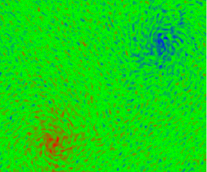
 where  $\boldsymbol{u}=(u_{x}(x,y),u_{y}(x,y),0)$ is the velocity field per unit mass, $\unicode[STIX]{x1D714}$ the non-vanishing component of its vorticity $\unicode[STIX]{x1D735}\times \boldsymbol{u}=(0,0,\unicode[STIX]{x1D714})$, $\unicode[STIX]{x1D708}$ the kinematic viscosity, $\unicode[STIX]{x1D6FC}\geqslant 0$ the Rayleigh damping coefficient and $\boldsymbol{f}$ a solenoidal body force. The subscripts $x$,
$x$,  $y$ and $z$ denote the respective components of a 3-D vector field.
We carry out direct numerical simulations of (2.1) on  $V=[0,2\unicode[STIX]{x03C0}]^{2}$ using the standard pseudospectral method (Orszag Reference Orszag1969) for spatial discretisation in conjunction with full dealiasing by truncation following the $2/3$rds rule (Orszag Reference Orszag1971). The initial data consist of random, Gaussian distributed vorticity fields. Owing to the focus on condensate formation and its dependence on large-scale friction, the friction coefficient $\unicode[STIX]{x1D6FC}$ was small or set to zero in some of the simulations. In the latter case the condensate saturates on a viscous time scale (Chan et al. Reference Chan, Mitra and Brandenburg2012; Linkmann et al. Reference Linkmann, Marchetti, Boffetta and Eckhardt2020) with the consequence that the simulations need to be evolved for a long time in order to obtain statistically stationary states. Similarly long transients occur for low values of $\unicode[STIX]{x1D6FC}$. As such, it was necessary to compromise on resolution, and the simulations were run using $256^{2}{-}512^{2}$ grid points.
In order to study the transitions, we conduct a parameter study for a stochastic, Gaussian distributed and  $\unicode[STIX]{x1D6FF}$-in-time correlated force $\boldsymbol{f}_{s}$ that is applied at scales corresponding to a wavenumber interval $[k_{min},k_{max}]$, and compare the results with those obtained with a forcing that is linear in the velocity field (Linkmann et al. Reference Linkmann, Boffetta, Marchetti and Eckhardt2019, Reference Linkmann, Marchetti, Boffetta and Eckhardt2020), i.e.
 $$\begin{eqnarray}\hat{\boldsymbol{f}}_{l}(\boldsymbol{k})=\unicode[STIX]{x1D708}_{IN}k^{2}\unicode[STIX]{x1D6FE}_{k}\hat{\boldsymbol{u}}(\boldsymbol{k}),\end{eqnarray}$$
 where  $\unicode[STIX]{x1D6FE}_{k}$ is a spherically symmetric Galerkin projector
 $$\begin{eqnarray}\unicode[STIX]{x1D6FE}_{k}=\left\{\begin{array}{@{}ll@{}}1\quad & \text{for }k\in [k_{min},k_{max}],\\ 0\quad & \text{otherwise}.\end{array}\right.\end{eqnarray}$$
 Here,  $k=|\boldsymbol{k}|$, while $\hat{\cdot }$ denotes the Fourier transform and $\unicode[STIX]{x1D708}_{IN}>0$ an amplification factor, such that the driving occurs through a linear instability in the wavenumber interval $[k_{min},k_{max}]$. The linear forcing is inspired by single-equation models describing dense bacterial suspensions (Wensink et al. Reference Wensink, Dunkel, Heidenreich, Drescher, Goldstein, Löwen and Yeomans2012; Słomka & Dunkel Reference Słomka and Dunkel2015; Linkmann et al. Reference Linkmann, Boffetta, Marchetti and Eckhardt2019, Reference Linkmann, Marchetti, Boffetta and Eckhardt2020), where active turbulence occurs. The latter is a spatio-temporally chaotic state characterised by the formation of mesoscale vortices owing to the collective effects of the microswimmers. These vortices occur in a narrow band of length scales, and can be described through a linear instability in the wavenumber interval $[k_{min},k_{max}]$ (Wensink et al. Reference Wensink, Dunkel, Heidenreich, Drescher, Goldstein, Löwen and Yeomans2012; Słomka & Dunkel Reference Słomka and Dunkel2015; Linkmann et al. Reference Linkmann, Marchetti, Boffetta and Eckhardt2020). Our previous studies (Linkmann et al. Reference Linkmann, Boffetta, Marchetti and Eckhardt2019, Reference Linkmann, Marchetti, Boffetta and Eckhardt2020), where linear forcing through a piecewise constant function as in (2.3) was introduced, were carried out in that context. In order to mimic the functional form of previously proposed single-equation models (Wensink et al. Reference Wensink, Dunkel, Heidenreich, Drescher, Goldstein, Löwen and Yeomans2012; Słomka & Dunkel Reference Słomka and Dunkel2015), which feature a hyperviscous term, an additional dissipation term $\unicode[STIX]{x1D708}_{2}\unicode[STIX]{x0394}\unicode[STIX]{x1D714}$ had been used at small scales, i.e. at $k>k_{min}$, resulting in the following equation
 $$\begin{eqnarray}\unicode[STIX]{x2202}_{t}\unicode[STIX]{x1D714}+(\unicode[STIX]{x1D714}\boldsymbol{\cdot }\unicode[STIX]{x1D735})\boldsymbol{u}=-\unicode[STIX]{x1D6FC}\unicode[STIX]{x1D714}+(\unicode[STIX]{x1D708}+\unicode[STIX]{x1D708}_{2})\unicode[STIX]{x0394}\unicode[STIX]{x1D714}+(\unicode[STIX]{x1D735}\times \boldsymbol{f}_{l})_{z},\end{eqnarray}$$
 where  $\unicode[STIX]{x1D708}_{2}>\unicode[STIX]{x1D708}$ for $k>k_{min}$ and zero otherwise.
For both  $\boldsymbol{f}_{s}$ and $\boldsymbol{f}_{l}$, statistically stationary states are eventually reached, where the spatio-temporally averaged energy dissipation, $\unicode[STIX]{x1D700}$, balances the spatio-temporally averaged energy input, $\unicode[STIX]{x1D700}_{IN}$,
 $$\begin{eqnarray}\unicode[STIX]{x1D700}:=\langle \unicode[STIX]{x1D700}(t)\rangle _{t}=\unicode[STIX]{x1D708}\langle \unicode[STIX]{x1D714}^{2}\rangle _{V,t}+\unicode[STIX]{x1D6FC}\langle |\boldsymbol{u}|^{2}\rangle _{V,t}=\langle \,\boldsymbol{f}\boldsymbol{\cdot }\boldsymbol{u}\rangle _{V,t}=\langle \unicode[STIX]{x1D700}_{IN}(t)\rangle _{t}=:\unicode[STIX]{x1D700}_{IN},\end{eqnarray}$$
 with  $\langle \cdot \rangle _{V,t}=\langle \langle \cdot \rangle _{V}\rangle _{t}$ denoting the combined spatial and temporal average. For Gaussian-distributed and $\unicode[STIX]{x1D6FF}(t)$-correlated random forcing, $\unicode[STIX]{x1D700}_{IN}$ is known a priori (Novikov Reference Novikov1965)
 $$\begin{eqnarray}{\unicode[STIX]{x1D700}_{IN}}_{s}=\langle \,\boldsymbol{f}_{s}\boldsymbol{\cdot }\boldsymbol{u}\rangle _{V,t}=\frac{F^{2}}{2},\end{eqnarray}$$
 where  $F=(\langle |\,\boldsymbol{f}_{\boldsymbol{s}}|^{2}\rangle _{V,t})^{1/2}$. That is, the energy input is a control parameter rather than an observable in simulations using $\boldsymbol{f}_{s}$. Details of the simulations are summarised in table 1.
For the linear forcing, the energy input is
 $$\begin{eqnarray}{\unicode[STIX]{x1D700}_{IN}}_{l}(t)=2(\unicode[STIX]{x1D708}_{IN}-\unicode[STIX]{x1D708})\int _{k_{min}}^{k_{max}}\,\text{d}k\,k^{2}E(k,t),\end{eqnarray}$$
where
 $$\begin{eqnarray}E(k,t)={\textstyle \frac{1}{2}}\int _{|\boldsymbol{k}|=k}\,\text{d}\boldsymbol{k}\,|\hat{\boldsymbol{u}}(\boldsymbol{k},t)|^{2},\end{eqnarray}$$
 is the energy spectrum. Equation (2.1) with  $\boldsymbol{f}=\boldsymbol{f}_{l}$ and the aforementioned enhanced small-scale damping has been solved numerically by Linkmann et al. (Reference Linkmann, Boffetta, Marchetti and Eckhardt2019, Reference Linkmann, Marchetti, Boffetta and Eckhardt2020) in the context of transitions to large-scale pattern formation in dense suspensions of active matter. Here, we compare our simulations listed in table 1 against the data of Linkmann et al. (Reference Linkmann, Boffetta, Marchetti and Eckhardt2019, Reference Linkmann, Marchetti, Boffetta and Eckhardt2020), as summarised in table 2. All simulations are evolved for several thousand large-eddy turnover times $\unicode[STIX]{x1D70F}=L/U$, where $U$ is the root-mean-square velocity and $L=2/U^{2}\int _{0}^{\infty }\text{d}kE(k)/k$ the integral length scale, with $E(k)=\langle E(k,t)\rangle _{t}$.
Table 1. Simulation details, where  $N$ is the number of grid points in each coordinate, $F$ the magnitude of the force acting in the interval $[k_{min},k_{max}]$ with $k_{min}=33$ and $k_{max}=40$ for all simulations, $\unicode[STIX]{x1D6FC}$ the large-scale friction parameter, $Re=UL/\unicode[STIX]{x1D708}$ the Reynolds number with respect to the root-mean-square velocity $U$, the integral length scale $L=2/U^{2}\int _{0}^{\infty }\text{d}kE(k)/k$ and the kinematic viscosity $\unicode[STIX]{x1D708}$. The latter was set to $\unicode[STIX]{x1D708}=0.0005$ for all simulations. The Reynolds number at the driven scales is $Re_{f}=U_{f}L_{f}/\unicode[STIX]{x1D708}$, with $U_{f}=(\int _{k_{min}}^{k_{max}}\text{d}kE(k))^{1/2}$ denoting the velocity at the driven scales and $L_{f}=2\unicode[STIX]{x03C0}/(k_{min}+k_{max})$. The large-eddy turnover time is denoted by $\unicode[STIX]{x1D70F}=L/U$.
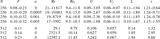
Table 2. Parameters used in DNSs using linear forcing and resulting observables (Linkmann et al. Reference Linkmann, Boffetta, Marchetti and Eckhardt2019, Reference Linkmann, Marchetti, Boffetta and Eckhardt2020). The number of grid points in each coordinate is denoted by  $N$, the viscosity by $\unicode[STIX]{x1D708}$, and $\unicode[STIX]{x1D708}_{IN}$, $k_{min}$, $k_{max}$ and $\unicode[STIX]{x1D708}_{2}$ are the parameters in (2.2)–(2.4). The Reynolds number $Re=UL/\unicode[STIX]{x1D708}$ is based on $\unicode[STIX]{x1D708}$, the root-mean-square velocity $U$ and the integral length scale $L=2/U^{2}\int _{0}^{\infty }\text{d}kE(k)/k$, with $\unicode[STIX]{x1D708}=1.1\times 10^{-3}$ for $N=256$ and $\unicode[STIX]{x1D708}=1.7\times 10^{-5}$ for $N=1024$. The Reynolds number at the driven scales is $Re_{f}=U_{f}L_{f}/\unicode[STIX]{x1D708}$, with $U_{f}=(\int _{k_{min}}^{k_{max}}\text{d}kE(k))^{1/2}$ denoting the velocity at the driven scales and $L_{f}=2\unicode[STIX]{x03C0}/(k_{min}+k_{max})$. The large-scale friction parameter $\unicode[STIX]{x1D6FC}=0$ and $(\unicode[STIX]{x1D708}+\unicode[STIX]{x1D708}_{2})/\unicode[STIX]{x1D708}=10$ for all simulations. Averages in the statistically stationary state are computed from at least 1800 snapshots separated by one large-eddy turnover time $\unicode[STIX]{x1D70F}=L/U$.

3 Random forcing
Before reporting on the results from the parameter study varying  $F$, we briefly discuss dynamical and statistical properties of the simulated flows using three example cases with $F=0.11$, $F=0.14$ and $F=0.23$. In order to facilitate the direct comparison with our previously published results using linear driving, the following presentation and discussion of the example cases is structured similarly to those discussed in Linkmann et al. (Reference Linkmann, Boffetta, Marchetti and Eckhardt2019, Reference Linkmann, Marchetti, Boffetta and Eckhardt2020).
Time series of the kinetic energy  $E(t)=\langle |\boldsymbol{u}|^{2}\rangle _{V}/2$ and visualisations of vorticity field samples taken during statistically steady evolution corresponding to the three example cases are shown in figure 1. For $F=0.23$ a condensate consisting of two counter-rotating vortices has formed. The remaining cases do not show large-scale structure formation. The time evolution of $E(t)$ and the representative vorticity fields of the three example cases are qualitatively similar to those obtained with linear forcing discussed in our previous work. Quantitative differences between the mean energy levels reported here and in Linkmann et al. (Reference Linkmann, Marchetti, Boffetta and Eckhardt2020) are due to the choice of parameter values. Please note that the example cases only serve to provide a qualitative overview of the data, which are discussed quantitatively in § 4.

Figure 1. (a) Time series for  $\unicode[STIX]{x1D6FC}=0$ and $F=0.11$ (blue), $F=0.14$ (purple) and $F=0.23$ (red). The data have been normalised with respect to the time-averaged energy for $F=0.11$, $E_{0}$, and the data for $F=0.23$ have been further divided by a factor 40 for presentational purposes. Time is given in units of large-eddy turnover time $\unicode[STIX]{x1D70F}$. (b) Corresponding visualisations of the respective vorticity fields during statistically stationary evolution.
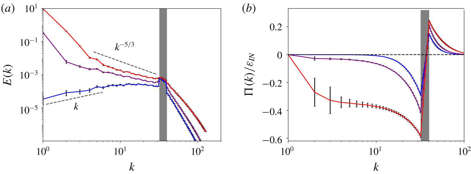
Figure 2. Energy spectra (a) and normalised fluxes (b) for  $\unicode[STIX]{x1D6FC}=0$ and $F=0.11$ (red), $F=0.14$ (purple) and $F=0.23$ (blue) for higher-resolved data in table 1. The grey-shaded area indicates the driving range. The error bars indicate the standard error calculated from statistically independent samples.
Figure 2 presents energy spectra (a) and normalised fluxes (b) for  $F=0.11$, $F=0.14$ and $F=0.23$. A scaling range characterised by a scaling exponent of the energy spectrum close to the Kolmogorov value $-5/3$ and a nearly wavenumber-independent flux only forms at the largest value of $F$. For smaller $F$ the flux tends to zero rapidly for $k<k_{min}$, hence dissipation cannot be negligible in this wavenumber range. In all cases the maximum and minimum values of the normalised flux do not add up to unity, which indicates that a substantial amount of energy is dissipated directly in the driving range. Interestingly, for intermediate values of $F$, the scaling exponent of the energy spectrum is still close but slightly larger than $-5/3$. For the smallest value of $F$ the energy spectrum scales linearly with $k$ for $k<7$, indicative of energy equipartition among Fourier modes in this wavenumber range. A similar transition in the energy spectra in statistically stationary 2-D turbulence occurs if the condensate is avoided through a strong drag term (Tsang & Young Reference Tsang and Young2009), in the sense that the extent of the $-5/3$ scaling range decreases with increasing large-scale friction and a power law with positive exponent appears at low wavenumbers. However, as a drag term alters the scale-by-scale energy balance, it breaks the zero-flux equilibrium condition that underlies linear scaling in two dimensions, the low-wavenumber scaling in the presence of drag is expected to differ from the absolute equilibrium scaling observed here for $\unicode[STIX]{x1D6FC}=0$. Indeed, in the former case the spectra are much steeper (Tsang & Young Reference Tsang and Young2009).
Condensates are known to affect inertial-range physics in terms of the properties of the third-order structure function (Xia et al. Reference Xia, Punzmann, Falkovich and Shats2008) and the scaling of the energy spectrum in the inertial range of scales (Chertkov et al. Reference Chertkov, Connaughton, Kolokolov and Lebedev2007). The spectral slopes observed here for the random forcing case and in the presence of a condensate are similar to those reported by Linkmann et al. (Reference Linkmann, Marchetti, Boffetta and Eckhardt2020) for the linearly forced case, hence the details of the small-scale forcing do not affect the spectral exponent. Deviations of the spectral exponent from the Kolmogorov value occur in a variety of turbulent systems. For a modified version of the Kuramoto–Sivashinski equation that allowed systematic deviations from inertial transfer, Bratanov et al. (Reference Bratanov, Jenko, Hatch and Wilczek2013) showed by semi-analytical and numerical means that non-universal power laws arise in spectral intervals where the ratio of linear and nonlinear time scales is wavenumber independent. As strong condensates result in a significant contribution of linear terms to the dynamics, a similar analysis could potentially lead to further insights on the non-universal scaling exponents in 2-D turbulence.
4 Non-universal transitions
The transition to 2-D turbulence as a function of the energy input has so far only been investigated for a single-equation model of active matter (Linkmann et al. Reference Linkmann, Boffetta, Marchetti and Eckhardt2019, Reference Linkmann, Marchetti, Boffetta and Eckhardt2020). Here, we now study the transition for a different kind of forcing and in the presence of large-scale friction, as condensates also occur in the presence of drag (Sommeria Reference Sommeria1986; Paret & Tabeling Reference Paret and Tabeling1998; Danilov & Gurarie Reference Danilov and Gurarie2001; Molenaar et al. Reference Molenaar, Clercx and van Heijst2004; van Heijst et al. Reference van Heijst, Clercx and Molenaar2006; Tsang & Young Reference Tsang and Young2009).
Figure 3(a) presents the shell-averaged amplitude of the lowest Fourier modes, i.e. the square root of the average energy at the largest scale,  $A_{1}=\sqrt{E(k)_{k=1}}$, as a function of $F$ from the parameter study for the random, Gaussian-distributed and $\unicode[STIX]{x1D6FF}(t)$-correlated forcing. Three main observations can be made from the figure 3(a). First, there is a clear transition point, below which $A_{1}\simeq 0$ and above which $A_{1}$ grows with increasing $F$, indicating the formation of a condensate and thus the onset of sustained inverse cascade, i.e. 2-D turbulence. Second, the data appear to be continuous at the critical point $F_{c}$ with a possibly discontinuous first derivative. The critical point is approached from above by a power law
 $$\begin{eqnarray}A_{1}\sim (F-F_{c})^{\unicode[STIX]{x1D6FE}},\end{eqnarray}$$
 where  $F_{c}=F_{c}(\unicode[STIX]{x1D6FC})$ and $\unicode[STIX]{x1D6FE}=\unicode[STIX]{x1D6FE}(\unicode[STIX]{x1D6FC})$ depend on the value of the large-scale friction coefficient. For $\unicode[STIX]{x1D6FC}=0$ the functional form $A_{1}(F)$ corresponds to the upper branch of the normal form of a supercritical pitchfork bifurcation, that is $\unicode[STIX]{x1D6FE}=1/2$. Third, for $F\gg F_{c}$ the amplitude $A_{1}$ grows linearly with $F$ in all cases. Equivalently, $E(k)_{k=1}$ grows linearly with $\unicode[STIX]{x1D700}_{IN}$, which is expected for a sizeable condensate as most of the dissipation should then take place at the largest scales
 $$\begin{eqnarray}\unicode[STIX]{x1D700}_{IN}=\unicode[STIX]{x1D700}=2\unicode[STIX]{x1D708}\int _{0}^{\infty }\text{d}k\,k^{2}E(k)+\unicode[STIX]{x1D6FC}\int _{0}^{\infty }\,\text{d}k\,E(k)\approx (2\unicode[STIX]{x1D708}+\unicode[STIX]{x1D6FC})E(k)_{|k=1}\unicode[STIX]{x1D6FF}k,\end{eqnarray}$$
 where  $\unicode[STIX]{x1D6FF}k$ is the grid spacing in Fourier space.
The dependence of  $F_{c}$ and $\unicode[STIX]{x1D6FE}$ on the large-scale friction coefficient $\unicode[STIX]{x1D6FC}$ is further quantified in figure 4. As can be seen in the figure, the approach to the critical point described by the exponent $\unicode[STIX]{x1D6FE}$, is strongly and nonlinearly dependent on the level of large-scale friction, while the location of the critical point varies little. A least-squares fit of $A_{1}$ against $F$ places the critical point at $F_{c}=0.135$ for $\unicode[STIX]{x1D6FC}=0$. For $\unicode[STIX]{x1D6FC}=0.0005$ we have $F_{c}=0.136$ and $\unicode[STIX]{x1D6FE}=0.72$, $\unicode[STIX]{x1D6FC}=0.001$ results in $F_{c}=0.138$ and $\unicode[STIX]{x1D6FE}=0.78$ and $\unicode[STIX]{x1D6FC}=0.005$ corresponds to $F_{c}=0.146$ and $\unicode[STIX]{x1D6FE}=1$. According to the discussion in the previous paragraph, $\unicode[STIX]{x1D6FE}=1$ is an asymptotic value in the sense that higher exponents are not expected.
The type of transition is very different if the driving occurs through a small-scale linear instability. Figure 3(b) presents the results of the parameter study carried out by Linkmann et al. (Reference Linkmann, Boffetta, Marchetti and Eckhardt2019, Reference Linkmann, Marchetti, Boffetta and Eckhardt2020) as a function of  $\unicode[STIX]{x1D708}_{IN}$ for the linear forcing specified in (2.2). In contrast to the randomly forced case, the transition is now subcritical (Linkmann et al. Reference Linkmann, Boffetta, Marchetti and Eckhardt2019, Reference Linkmann, Marchetti, Boffetta and Eckhardt2020) as evidenced by a discontinuity in the data and the clearly visible hysteresis loop. The latter is discussed by Linkmann et al. (Reference Linkmann, Marchetti, Boffetta and Eckhardt2020) in further detail, with figure 3 showing the same result as figure 5 of the aforementioned publication, using $A_{1}$ instead of $E(k)_{|k=1}$. As the hysteresis loop is small, one may expect that the transitions happen at comparable values of a forcing-scale Reynolds number $Re_{f}=U_{f}L_{f}/\unicode[STIX]{x1D708}$, where $L_{f}$ is a length scale that corresponds to the middle wavenumber in the driven range, $L_{f}=2\unicode[STIX]{x03C0}/(k_{min}+k_{max})$, and $U_{f}$ is the root-mean-square velocity in that range of scales
 $$\begin{eqnarray}U_{f}=\left(\int _{k_{min}}^{k_{min}}\text{d}k\,E(k)\right)^{1/2}.\end{eqnarray}$$
 This is indeed the case, the transition occurs at  $Re_{f}\approx 20$ in the subcritical case (Linkmann et al. Reference Linkmann, Boffetta, Marchetti and Eckhardt2019) and at $Re_{f}\approx 10$ in the supercritical case studied here.

Figure 3. Shell-averaged amplitude of the Fourier modes at the largest scale,  $A_{1}=\sqrt{E(k)_{k=1}}$, as a function of $F$ for random forcing (a) and $\unicode[STIX]{x1D708}_{IN}$ for linear forcing (b).

Figure 4. Dependence of the critical point  $F_{c}$ (a) and the exponent $\unicode[STIX]{x1D6FE}$ (b) on the large-scale damping coefficient $\unicode[STIX]{x1D6FC}$. The error bars show the error of the fit (one standard deviation).
Non-universality in the transition to condensate formation also occurs in the Gross–Pitaevsky model of wave turbulence: for small-scale driving by a local-in-scale linear instability, a series of symmetry-breaking sharp transitions occur as function of increasing wave action (Vladimirova et al. Reference Vladimirova, Derevyanko and Falkovich2012). The first statistical symmetry that breaks with increasing condensate growth is isotropy, followed by twofold, threefold and fourfold symmetries. Interestingly, such symmetry breaking does not occur if the driving is realised through a small-scale random process. That is, final turbulent states with different statistical symmetries are obtained for different types of small-scale energy input. In weak turbulence, differences between turbulent states originating from the type of driving arise in the context of information theory through different entropy extraction rates (Falkovich & Shavit Reference Falkovich and Shavit2019). As a non-equilibrium steady state, turbulence is a driven-dissipative system, that is, its phase-space measure will be non-uniform, detailed balance is broken and the information-theoretic entropy of that measure (here, the differential entropy of the phase-space measure with respect to the Lebesgue measure) becomes time dependent. Only driving and dissipation contribute to this time dependence, and Falkovich & Shavit (Reference Falkovich and Shavit2019) showed that the rate of change in (differential) entropy depends explicitly on the phase-space measure for random forcing while it is independent thereof if the driving is given by a local-in-scale linear instability. In other words, the information context of the system depends on the type of driving, which may be expected, especially concerning comparisons with random forcing. Here, we did not observe any difference in statistical symmetry between randomly forced 2-D turbulence and 2-D turbulence generated by a small-scale instability, however, this may well be because the condensates attained here and in our previous work are moderate in amplitude.
5 Conclusions
We here study the formation of the condensate and thereby the transition to 2-D turbulence as a function of the type and amplitude of the forcing. Direct numerical simulations show that the condensate does not appear gradually but in a phase transition. For prescribed energy dissipation the transition is second order, and both the critical point and the critical exponent depend on the value of the large-scale friction coefficient. In this context, we point out that  $\unicode[STIX]{x1D700}$ does not depend on $\unicode[STIX]{x1D6FC}$ for the random, $\unicode[STIX]{x1D6FF}(t)$-correlated forcing used here, as is the case for time-independent forcing such as Kolmogorov flow (Tsang & Young Reference Tsang and Young2009). However, a series of test simulations using time-independent forcing led to similar results (S. Musacchio & G. Boffetta, private communication). When the forcing is due to a small-scale instability as inspired by continuum models of active matter, the transition is first order (Linkmann et al. Reference Linkmann, Boffetta, Marchetti and Eckhardt2019, Reference Linkmann, Marchetti, Boffetta and Eckhardt2020). The phase transitions separate two markedly different types of 2-D dynamics: in 2-D turbulence, energy input is predominantly balanced by large-scale dissipation either in the condensate or through Rayleigh friction, and intermediate scales follow an inertial cascade; in spatio-temporally chaotic states where no condensation occurs, dissipation is spread over the intermediate scales and the properties of the energy transfer are noticeably different and non-universal.
In summary, the transition to 2-D turbulence is non-universal in the sense that (i) the type of transition depends on the type of forcing, and (ii) the details of the transition for a given type of forcing depend on other system parameters such as large-scale friction. The presence of these non-universalities naturally motivates questions concerning their origin. Results from rapidly rotating Rayleigh–Bénard convection (Favier et al. Reference Favier, Guervilly and Knobloch2019) suggest that the hysteretic transition in the linearly forced case may be related to persistent phase correlations between the driven scales and the condensate. Random forcing precludes such a scenario. Further questions concern the theoretical predictions on the dependence of the critical exponent  $\unicode[STIX]{x1D6FE}$ on the level of large-scale friction. The value $\unicode[STIX]{x1D6FE}=1$ is plausible for strong linear damping by the same argument that predicted a linear dependence of the energy in the condensate on the energy input. Finally, it remains to be seen if symmetry-breaking transitions between condensates as in the Gross–Pitaevsky equation (Vladimirova et al. Reference Vladimirova, Derevyanko and Falkovich2012) also occur for the 2-D Navier–Stokes equations.
Acknowledgements
B.E. sadly passed away before the manuscript was written. We hope to have summarised the collaborative work according to his standards, and any shortcomings should be attributed to M.L. We will remember him as an outstanding scientist, thoughtful supervisor and inspiring role model. M.L. thanks G. Boffetta and S. Musacchio for helpful discussions and the anonymous referees for their suggestions, which have significantly improved the quality of this manuscript.
Declaration of interests
The authors report no conflict of interest.


 Open access