


1. Introduction
In inviscid linear theory, waves propagating through stratified, horizontally directed and sheared flow encounter singularities at a novel type of critical level. These ‘baroclinic’ critical levels arise where the phase speed relative to the basic flow matches a characteristic gravity wavespeed (Olbers Reference Olbers1981; Basovich & Tsimring Reference Basovich and Tsimring1984; Badulin, Shrira & Tsimring Reference Badulin, Shrira and Tsimring1985; Staquet & Huerre Reference Staquet and Huerre2002; Boulanger, Meunier & Le Dizès Reference Boulanger, Meunier and Le Dizès2008; Wang & Balmforth Reference Wang and Balmforth2018, Reference Wang and Balmforth2020). Much like the classical critical level, the singularity must be resolved by weak viscosity, unsteadiness or nonlinearity. However, disturbances typically remain strong in the vicinity of the singular levels, the baroclinic critical layers, with potentially important implications for mixing and the transition to turbulence.
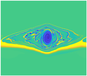
In previous work (Wang & Balmforth Reference Wang and Balmforth2020), we studied the nonlinear evolution of the baroclinic critical layers of a wave driven by a steady wavemaker into the rotating, uniformly stratified, Couette flow illustrated in figure 1. The initial, linear dynamics that arises is similar to that for internal gravity waves (Booker & Bretherton Reference Booker and Bretherton1967; Brown & Stewartson Reference Brown and Stewartson1980) or Rossby waves (Stewartson Reference Stewartson1978; Warn & Warn Reference Warn and Warn1978): disturbances grow secularly over a gradually narrowing critical layer. Modifications to the mean flow, with the form of a jet-like defect, then come into play to terminate the linear growth, whilst still allowing further sharpening of the density gradients within even thinner regions inside the critical layer. This later-time dynamics is very different to that occurring inside the critical layer of a forced Rossby wave, where the local vorticity field rolls up into a distinctive cat's eye pattern (Stewartson Reference Stewartson1978; Warn & Warn Reference Warn and Warn1978).

Figure 1. Sketch of the model. A wavemaker with wavenumbers  $k_x$ and $k_z$ is introduced at $y=0$, forcing the baroclinic critical levels at $y=\pm N/(\varLambda k_x)$ (corresponding to dimensionless locations $\pm \mathcal {N}$ with ${\mathcal {N}}=N\varLambda ^{-1}$) and leading to defects in the mean flow. Small perturbations in vertical vorticity near $y=N/(\varLambda k_x)$ then seed a secondary instability that induces the roll up of the defect there, creating a new wave with a different phase speed that forces a new set of of baroclinic critical levels.
In the current paper, we take our analysis of forced baroclinic critical layers in a different direction: jet-like defects embedded within linear shear are expected in general to modify the stability of a flow by introducing inflexion points into the mean velocity profile (Gill Reference Gill1965; Lerner & Knobloch Reference Lerner and Knobloch1988; Balmforth, Castillo-Negrete & Young Reference Balmforth, del Castillo-Negrete and Young1997). This leads one to suspect that the mean-flow modification incurred inside the baroclinic critical layer suffers secondary instabilities (see also Umurhan, Shariff & Cuzzi Reference Umurhan, Shariff and Cuzzi2016). Indeed, Killworth & McIntyre (Reference Killworth and McIntyre1985) and Haynes (Reference Haynes1985, Reference Haynes1989) have shown that the cat's eye in the Rossby-wave critical layer is susceptible to secondary instabilities, owing to the introduction of local reversals of the mean vorticity gradient. Similarly, Boulanger et al. (Reference Boulanger, Meunier and Le Dizès2008) have argued that secondary instabilities in viscous, baroclinic critical layers rationalize the emergence of strong vertical motions in tilted stratified vortices.
To delve more deeply into this question, we draw a parallel with our previous study and exploit a matched asymptotic expansion to derive a reduced model that captures the secondary instability of the forced baroclinic critical layer. The key difference with our earlier exploration is that vorticity gradient associated with the mean defect becomes order one at an earlier time than the mean-flow modification feeds back upon the secularly growing critical-layer disturbance. In other words, secondary instabilities may become possible before nonlinearity arrests the linear growth. Such relatively fast instabilities are filtered over the longer-time dynamics of our original asymptotic expansion. A different critical-layer theory is therefore required, one that turns out to be more like conventional analyses of classical critical layers (Stewartson Reference Stewartson1978; Warn & Warn Reference Warn and Warn1978). The reduced model provides us with a compact formalism to detect secondary instability and explore the consequences. In particular, we provide a linear stability theory for the defect, taking into account the time dependence of the basic state explicitly by solving the corresponding initial-value problem (which also provides a gauge for the accuracy of a frozen-time normal-mode approximation). We then solve the reduced model numerically to explore the nonlinear dynamics of the secondary instability.
A main issue is whether the dynamics of the forced baroclinic critical layer and its secondary instability bears upon the self-replication of vortices observed in numerical simulations by Marcus et al. (Reference Marcus, Pei, Jiang and Hassanzadeh2013, Reference Marcus, Pei, Jiang and Barranco2015, Reference Marcus, Pei, Jiang and Barranco2016). In particular, imagining our original wavemaker to represent a localized vortex seeded in the shear flow, the issue is whether secondary instability can induce a roll up of the defects inside the baroclinic critical layers to create new vortices that can in turn act as new wavemakers. Provided the new vortices are sufficiently strong to initiate a self-perpetuating cycle, we may provide a theoretical underpinning for the numerical observations. We return to this particular motivating issue in our concluding discussion.
The organization of the paper is as follows. In § 2, we give the mathematical model and briefly review our previous paper: we show the secular growth of linear waves in the critical layer, which then forces a mean-flow defect. Then we diverge from our previous paper in studying the mean flow's nonlinear feedback to the fundamental wave, and instead, we embark on a new route of exploring the secondary instability induced by the mean-flow defect. In § 3, we use the method of matched asymptotic expansions to build a reduced model which compactly describes the leading-order dynamics of the secondary instability. We solve the linear instability problem analytically in § 4, emphasizing its unusual properties endowed by the unsteadiness of the mean-flow defect. The subsequent nonlinear evolution is solved numerically in § 5, showing the defect rolling up into vortices, and we also give a comment on how the secondary instability could enable the replication of zombie vortices. Discussion and concluding remarks are given in § 6.
2. Mathematical formulation and background
2.1. Model and governing equations
As sketched in figure 1, the basic flow has a horizontal velocity  $U=\varLambda y$ pointing in the $x$-direction, with a shear rate $\varLambda$ in the $y$-direction. The fluid has reference density $\rho _0$ and is uniformly stratified with buoyancy frequency $N$. The domain rotates around the vertical $z$-axis at rate $\varOmega$. A steady wavemaker with horizontal and vertical wavenumbers $k_x$ and $k_z$ is imposed at $y=0$. We define the dimensionless parameters $\mathcal {N}=N/\varLambda$ and $f=2\varOmega /\varLambda$, and non-dimensionalize the length, time, velocity, pressure and density by $k_x^{-1}$, $\varLambda ^{-1}$, $\varLambda k_x^{-1}$, $\rho _0\varLambda ^2/(k_xg)$ and $\rho _0\varLambda ^2/(k_xg)$, respectively, where g is the gravitational acceleration. If ( $u,v,w,\rho,p$) represent the perturbations to the three velocity components, density and pressure imposed on the basic state, the governing equations are
 \begin{gather} u_t+yu_x+(1-f)v+uu_x+vu_y+wu_z={-}p_x+{\tilde\nu} \nabla^2u, \end{gather}
 \begin{gather}v_t+yv_x+fu+uv_x+vv_y+wv_z={-}p_y+{\tilde\nu} \nabla^2v, \end{gather}
 \begin{gather}w_t+yw_x+uw_x+vw_y+ww_z={-}p_z-\rho+{\tilde\nu} \nabla^2w, \end{gather}
 \begin{gather}\rho_t+y\rho_x-{\mathcal{N}}^2 w+u\rho_x+v\rho_y+w\rho_z={\tilde\chi} \nabla^2\rho-{\tilde\lambda}\rho, \end{gather}
 \begin{gather}u_x+v_y+w_z=0, \end{gather}
where the  $(x,y,z,t)$ subscripts represent partial derivatives, and viscosity and diffusion of density perturbations (i.e. temperature) are included, with dimensionless strengths of ${\tilde \nu }$ and ${\tilde \chi }$ (the dimensional kinematic viscosity and diffusivity scaled by $\varLambda /k_x^2$). In view of astrophysical applications, we focus on the limit where ${\tilde \nu }$ and ${\tilde \chi }$ are small, and also include a term representing Newton cooling in (2.4), with parameter ${\tilde \lambda }$. An equation for the vertical component of vorticity follows from (2.1) and (2.2):
 \begin{align} \left[\frac{\partial}{\partial t}+(y+u)\frac{\partial}{\partial x} +v\frac{\partial}{\partial y}+w\frac{\partial}{\partial z} - w_z - {\tilde\nu} \nabla^2 \right](v_x-u_y+f-1)+w_xv_z-w_yu_z= 0. \end{align}
 To continuously force waves into the system, we introduce an idealized wavemaker at  $y=0$. Booker & Bretherton (Reference Booker and Bretherton1967), Stewartson (Reference Stewartson1978) and Warn & Warn (Reference Warn and Warn1978) all adopted a wavy boundary for this task. Here, however, we adopt a different forcing more equivalent to the initialization of the simulations by Marcus et al. In particular, we place a localized strip of vorticity at $y=0$ that introduces a jump in the tangential velocity but leaves the normal velocity continuous:
 \begin{equation} u|_{y=0+}- u|_{y=0-} =\varepsilon_0\exp(\mathrm{i}x+\mathrm{i}mz)+\mathrm{c.c.},\quad v|_{y=0+}=v|_{y=0-}, \end{equation}
where  $\varepsilon_0$ is a small number representing the strength of the forcing, m is the ratio of vertical to horizontal wavenumbers, and c.c. represents the complex conjugate.
The forcing is switched on at
$\varepsilon_0$ is a small number representing the strength of the forcing, m is the ratio of vertical to horizontal wavenumbers, and c.c. represents the complex conjugate.
The forcing is switched on at  $t=0$, and remains fixed throughout, with our main objective being to study the evolution of the baroclinic critical layers that are thereby forced. Consequently, we ignore any structure and the evolution of the forcing itself; we return to this limitation and its possible impacts in our conclusions.
The disturbances are assumed to decay for  $|y|\gg 1$ and satisfy periodic boundary conditions in $x$ and $z$; in practice, we assume the same periodicity as the forcing. As in Wang & Balmforth (Reference Wang and Balmforth2020), we assume that the flow is linearly stable: we take $f(f-1)>0$ to eliminate the centrifugal instability (Emanuel Reference Emanuel1994); the lack of any reflective boundaries removes the possibility of the strato-rotational instability (Vanneste & Yavneh Reference Vanneste and Yavneh2007; Wang & Balmforth Reference Wang and Balmforth2018).
2.2. The linear non-dissipative baroclinic critical layer
In inviscid, non-diffusive linear theory, we neglect all the nonlinear and dissipative terms in (2.1)–(2.5). Outside the baroclinic critical layers surrounding  $y=\pm \mathcal {N}$, the flow is characterized by a steady wave solution of the form,
 \begin{equation} (u,v,w,p,\rho)=\varepsilon[\hat{u}_\mathrm{I}(y),\hat{v}_\mathrm{I}(y), \hat{w}_\mathrm{I}(y),\hat{p}_\mathrm{I}(y),\hat{\rho}_\mathrm{I}(y)] \exp({\mathrm{i}x+\mathrm{i}mz}) +\mathrm{c.c.}, \end{equation}
where the amplitudes, identified by the subscript ‘I’, satisfy a second-order differential equation (Wang & Balmforth Reference Wang and Balmforth2020). However, the solution remains time dependent near the critical levels. Focusing on the level at  $y={\mathcal {N}}$, one finds
 \begin{equation} p\rightarrow \varepsilon A\exp({\mathrm{i}x+\mathrm{i}mz})+\mathrm{c.c.}, \quad \textrm{for}\ y\rightarrow \mathcal{N}, \end{equation}
where  $\varepsilon$, related to $\varepsilon _0$, gauges the strength of the forcing at the baroclinic critical layer, so that $|A|=1$ and $A$ encodes a complex phase dictated by $\hat {p}_\mathrm {I}(y)$ (Wang & Balmforth Reference Wang and Balmforth2020). The remainder of the time-dependent solution near this particular critical level depends on the rescaled variables,
 \begin{equation} Y=\frac{y-\mathcal{N}}{\delta},\quad T=\delta t \end{equation}
where  $\delta$ is a small parameter measuring the length scale of the critical layer, such that
 \begin{align} \left(u,v,w,\rho
\right)=\varepsilon[u_\mathrm{I}(Y,T),v_\mathrm{I}(Y,T),
\delta^{{-}1}
w_\mathrm{I}(Y,T),\delta^{{-}1}\rho_\mathrm{I}(Y,T)]
\exp({\mathrm{i}x+\mathrm{i}mz})+\mathrm{c.c.}
\end{align}
\begin{align} \left(u,v,w,\rho
\right)=\varepsilon[u_\mathrm{I}(Y,T),v_\mathrm{I}(Y,T),
\delta^{{-}1}
w_\mathrm{I}(Y,T),\delta^{{-}1}\rho_\mathrm{I}(Y,T)]
\exp({\mathrm{i}x+\mathrm{i}mz})+\mathrm{c.c.}
\end{align}
Substituting into the linear, non-dissipative versions of (2.3) and (2.4), we obtain, to leading order
 \begin{equation} \left(\frac{\partial}{\partial T}+\mathrm{i}Y\right)\rho_\mathrm{I} ={-}\frac{1}{2}m{\mathcal{N}} A,\quad w_1=\frac{\mathrm{i}}{\mathcal{N}} \rho_\mathrm{I}. \end{equation}
With the initial condition,  $\rho _\mathrm {I}\rightarrow 0$ as $T\rightarrow 0$, we solve (2.12a,b) to obtain
 \begin{equation} \rho_\mathrm{I} = \frac{1}{2} \textrm{i} m {\mathcal{N}} A \frac{1-\textrm{e}^{-\mathrm{i}YT}}{Y} . \end{equation}
This solution illustrates the linear growth of the density and vertical velocity perturbations over an increasingly narrow critical layer with  $Y=O( T^{-1})$ or $y={\mathcal {N}}+O(t^{-1})$. From the leading order of (2.5) and (2.1), we further derive
 \begin{equation} v_{\mathrm{I}Y}={-}\mathrm{i}mw_\mathrm{I},\quad u_\mathrm{I}= \frac{\mathrm{i}(1-f)v_\mathrm{I}-A}{\mathcal{N}}. \end{equation}
The second critical layer at  $y=-{\mathcal {N}}$ is treated similarly, with the spatial symmetry of the problem ensuring that no separate considerations are required (Wang & Balmforth Reference Wang and Balmforth2020). Note that $\delta$ is not prescribed for this derivation (and, indeed, (2.11) is independent of $\delta$ when expressed in terms of $t$ and $y$); this scale becomes selected, however, in the developments of § 3. Also, in (2.14a,b) and below, we extend our shorthand subscript notation for derivatives to $Y$,
$Y$,  $T$, a rescaled coordinate $\xi$ and a phase variable $\theta$.
2.3. The mean-flow response in a non-dissipative critical layer
To find the mean-flow response within the critical layer at  $y={\mathcal {N}}$, we set
 \begin{align} (u,v,w,\rho,p) &= \varepsilon [u_\mathrm{I}(Y,T),v_\mathrm{I}(Y,T),\delta^{{-}1}w_\mathrm{I}(Y,T), \delta^{{-}1}\rho_\mathrm{I}(Y,T),p_\mathrm{I}(Y,T)] \nonumber\\ &\quad \times \exp({\mathrm{i}x+\mathrm{i}mz})+\mathrm{c.c.} \nonumber\\ &\quad +\varepsilon^2[\delta^{{-}2}u_0(Y,T),0,\delta^{{-}2}w_0(Y,T),\delta^{{-}2}\rho_0(Y,T),p_0(Y,T)]+\cdots, \end{align}
where spatial periodicity in  $x$ and $z$ and the decay for $|y|\gg 1$ removes any mean-flow component to $v$, and the omitted terms include an $O({\varepsilon }^2)$ first harmonic and higher-order corrections (cf. Wang & Balmforth Reference Wang and Balmforth2020). Substituting (2.15) into (2.1)–(2.5) and extracting the mean-flow components, we find
 \begin{equation} \left.\begin{gathered} u_{0T} = \textrm{i}mw_\mathrm{I}u_\mathrm{I}^*-v_\mathrm{I}^*u_{\mathrm{I}Y} +\mathrm{c.c.},\quad p_{0Y} = \textrm{i}mw_\mathrm{I}v_\mathrm{I}^* - v_\mathrm{I}^* v_{\mathrm{I}Y}+\mathrm{c.c.},\\ \rho_0 ={-} v_\mathrm{I}^*w_{\mathrm{I}Y}+\mathrm{c.c.},\quad - {\mathcal{N}}^2 w_0 ={-} v_\mathrm{I}^*\rho_{\mathrm{I}Y}+\textrm{i}mw_\mathrm{I}^*\rho_\mathrm{I}+\mathrm{c.c.} \end{gathered}\right\} \end{equation}
Substituting (2.13) and (2.14a,b) into (2.16a) and then integrating now yields
 \begin{equation} u_0= \frac{m^2}{\mathcal{N}}\frac{\cos YT-1}{Y^2}. \end{equation}
Wang & Balmforth (Reference Wang and Balmforth2020) show that when  $t=O(\varepsilon ^{-{2}/{3}})$ and $\delta =\varepsilon ^{2/3}$, the mean flow feeds back on to the linear solution (2.13), halting the secular growth. However, in the next section, we will see that a secondary instability can arise for earlier times, and, in particular, when the mean vorticity gradient becomes order one. From (2.17), we see that this demands that ${\varepsilon }^2\delta ^{-2} u_{0yy} = O({\varepsilon }^2 \delta ^{-4}) = O(1)$, or $\delta = {\varepsilon }^{1/2}$, which sets the stage for our matched asymptotic analysis.
3. The reduced model
As indicated above, the structure of the solution consists of an outer region, in which the  $O({\varepsilon })$ disturbance forced by the wavemaker is quasi-steady, that is coupled to inner regions of thickness $O({\varepsilon }^{1/2})$ surrounding the baroclinic critical levels where evolution takes place over an $O({\varepsilon }^{-1/2})$ time scale. We further take the distinguished limit in which the dissipative terms only enter the problem within the critical layers where the fine length scale and slower time promote their importance, leading us to the rescalings
 \begin{equation} {\tilde\nu} = {\varepsilon}^{{3}/{2}} {\nu},\quad {\tilde\chi} = {\varepsilon}^{{3}/{2}} {\chi} \quad \textrm{and} \quad {\tilde\lambda} = 2{\varepsilon}^{1/2} {\lambda}. \end{equation}
 As in Wang & Balmforth (Reference Wang and Balmforth2020), the problem possesses an important symmetry about  $y=0$. For the forced wave, with its two baroclinic critical levels at $y=\pm {\mathcal {N}}$, the symmetry allows us to consider the spatial half of the problem in $y>0$ and thereby focus on only one of the critical layers. In the secondary instability problem, however, each of the defects generated at these levels can act as the seed of secondary instability. The problem is conveniently simplified by focusing on only one of the defects and considering the disturbances that amplify in its vicinity as a result of a suitable initial perturbation (cf. figure 1). In this situation, the secondary instability is purely driven by the defect at $y=+{\mathcal {N}}$ and develops no fine structure near $y=-{\mathcal {N}}$. In other words, there is only one effective defect for the secondary instability. Moreover, because the basic flow velocity is $\mathcal {N}$ at the defect, the associated phase velocity of the secondary instability must be $\mathcal {N}$ to leading order, a detail that also follows from the leading-order balances in the critical layer, and is standard for instability induced by localized defects (Gill Reference Gill1965; Balmforth et al. Reference Balmforth, del Castillo-Negrete and Young1997).
3.1. Outer solution
We first consider the evolution of secondary instability in the outer region, i.e. away from the critical level  $y=\mathcal {N}$. Since the instability is primarily generated by the localized defect, the outer solution features linear quasi-steady waves with phase velocity $\mathcal {N}$ and slowly evolving amplitudes driven by the critical-layer disturbances. The nonlinearity within the critical layer also generates a broad spectrum of linear waves for the outer flow. We therefore set
 \begin{align} (u,v,w,\rho,p) &= \varepsilon[\hat{u}_\mathrm{I}(y),\hat{v}_\mathrm{I}(y), \hat{w}_\mathrm{I}(y),\hat{p}_\mathrm{I}(y), \hat{\rho}_\mathrm{I}(y)]\exp({\mathrm{i}x+\mathrm{i}mz}) \nonumber\\ &\quad +\varepsilon\sum_{n=1}^{\infty}\varPhi_{n}(T) [\hat{u}_n(y),\hat{v}_n(y),\hat{w}_n(y),\hat{\rho}_n(y),\hat{p}_n(y)] \exp({\mathrm{i}n{\scriptscriptstyle K}\theta})+\mathrm{c.c.}, \end{align}
where the second instability is characterized by the phase,
 \begin{equation} \theta=x+mz-\mathcal{N}t, \end{equation}
and the amplitude  $\varPhi _n$ of the $n$th wave component. The wavenumber factor ${\scriptstyle K}$ allows the secondary instability to have a different fundamental wavelength ( $2{\rm \pi} /{\scriptstyle K}$) than the forcing, although, for simplicity, we restrict the vertical wavenumber to be the same multiple $m$ of the horizontal wavenumber as the forcing. Given the instability is mainly caused by horizontal shear, this restriction does not seem particularly limiting and we expect similar results had we considered other vertical wavenumbers.
The spatial dependence of the outer solution is given by the linear steady wave equation
 \begin{equation} {P}_{\xi\xi}-\frac{2\xi{P}_\xi }{\xi^2-f(f-1)}- \left[\frac{\xi^2-f(f+1)}{\xi^2-f(f-1)}+ m^2\frac{\xi^2-f(f-1)}{\xi^2-\mathcal{N}^2}\right]{P}=0, \end{equation}
with  $\hat {p}_n(y)={P}(\xi )$,
 \begin{equation} \xi = n{\scriptstyle K}(y-{\mathcal{N}}) \end{equation}
and
 \begin{equation} \left.\begin{gathered} \hat{u}_n=\frac{n{\scriptstyle K}[(f-1){P}_\xi-\xi{P}]}{\xi^2-f(f-1)},\quad \hat{v}_n=\frac{\mathrm{i}n{\scriptstyle K}[\xi{P}_\xi-f{P}]}{\xi^2-f(f-1)},\\ \hat{w}_n={-}\frac{nm{\scriptstyle K}\xi{P}}{\xi^2-\mathcal{N}^2},\quad \hat{\rho}_n=\frac{\mathrm{i}nm{\scriptstyle K}\mathcal{N}^2{P}}{\xi^2-\mathcal{N}^2}. \end{gathered}\right\} \end{equation}
But for the replacement of  $y$ by $\xi$, (3.4) is identical to the equation that must be solved to determine the outer solution $\hat {p}_\mathrm {I}(y)$ for the original, quasi-steady forced wave (Wang & Balmforth Reference Wang and Balmforth2020). Here, however, we solve this equation with conditions specific to the secondary instability imposed at $y={\mathcal {N}}$ ( $\xi =0$; the distinguished defect) and the singular points of (3.4). The latter are located at the positions where the coefficients in (3.4) diverge, namely $\xi ^2=f(f-1)$ and $\xi ^2={\mathcal {N}}^2$. The divergences at $\xi =\pm \sqrt {f(f-1)}$ (which are real, given our assumption that $f(f-1)>0$) correspond to removable singular points (cf. Vanneste & Yavneh Reference Vanneste and Yavneh2007; Wang & Balmforth Reference Wang and Balmforth2020) and require no special attention. The singular points at $\xi =\pm {\mathcal {N}}$ are genuine and correspond to $y = {\mathcal {N}} [1 \pm (n{\scriptstyle K})^{-1}]$; these are the new baroclinic critical levels of the outer (quasi-steady) wave characterizing the secondary instability, which are displaced from the original baroclinic critical level and defect at $\xi =0$ ( $y={\mathcal {N}}$) owing to the different phase speed (see figure 1 and (3.2)).
More specifically, we solve (3.4) subject to the far-field conditions  ${P}(\xi )\to 0$ for $\xi \to \pm \infty$, together with matching conditions at both the defect ( $\xi =0$) and the new baroclinic critical levels $\xi =\pm {\mathcal {N}}$. Importantly, the dynamics at the new baroclinic levels follows the same pattern as the forced wave at the original baroclinic levels. In particular, for the time scale and amplitude on which the secondary instability develops, that dynamics remains linear and can be understood by a similar analysis to that in § 2.2, or its dissipative generalization. This consideration leads us to demand that ${P}(\xi )$ be continuous at $\xi =\xi _B=\pm {\mathcal {N}}$, but suffers a jump in derivative given by
 \begin{equation} \textrm{Lim}_{\epsilon\to0}[{P}_\xi]_{\xi_B-\epsilon}^{\xi_B+\epsilon} = \frac{\mathrm{i}{\rm \pi} m^2[{\mathcal{N}}^2-f(f-1)]}{2\xi_B} {P}(\xi_B),\end{equation}
in the manner of the Lin rule commonly employed for classical critical levels (Lin Reference Lin1945) and irrespective of whether there is dissipation or not. Salient details of the calculation are provided in Appendix A. Note that this condition ensures that  ${P}(\xi )$ is independent of $n$, other than through the rescaled coordinate $\xi \equiv n{\scriptstyle K}(y-{\mathcal {N}})$.
By contrast, we must deal with a fully nonlinear critical layer at the defect once the secondary instability emerges, which translates to a non-trivial matching condition. To pave the way for this matching, we observe the limits,
 \begin{equation} \hat{p}_n= {P} \to
\left\{ \begin{array}{@{}ll@{}} (f-1)[1+\alpha_{+}\xi+\cdots],
& \xi>0 \ \textrm{or} \ y>\mathcal{N},
\\ (f-1)[1+\alpha_{-}\xi+\cdots], &
\xi<0 \ \textrm{or} \ y<\mathcal{N},
\end{array}\right. \end{equation}
\begin{equation} \hat{p}_n= {P} \to
\left\{ \begin{array}{@{}ll@{}} (f-1)[1+\alpha_{+}\xi+\cdots],
& \xi>0 \ \textrm{or} \ y>\mathcal{N},
\\ (f-1)[1+\alpha_{-}\xi+\cdots], &
\xi<0 \ \textrm{or} \ y<\mathcal{N},
\end{array}\right. \end{equation}
and
 \begin{align} v \to \varepsilon\sum_{n=1}^\infty\mathrm{i}n{\scriptstyle K}\varPhi_n\exp({\mathrm{i}n{\scriptscriptstyle K}\theta})+\mathrm{c.c.},\quad u\rightarrow \varepsilon\sum_{n=1}^\infty n{\scriptstyle K}\varPhi_n\frac{1-f}{f} \alpha_{{\pm}}\exp({\mathrm{i}n{\scriptscriptstyle K}\theta})+\mathrm{c.c}. \end{align}
The coefficients  $\alpha _\pm$ follow from the solution of (3.4) with the far-field conditions and (3.7). A sample solution for $P(\xi )$ is shown in figure 2.

Figure 2. The outer quasi-steady wave solution  $P(\xi )$ of the secondary instability, $m=1/2$, $\mathcal {N}=4/3$, $f=4/3$.
3.2. Inner region
The inner region has a length scale  $O(\varepsilon ^{{1}/{2}})$ surrounding the critical level $y=\mathcal {N}$, and evolves in a slow time scale of $O(\varepsilon^{-1/2})$. Therefore, we introduce the rescalings
 \begin{equation} T=\varepsilon^{{1}/{2}}t,\quad Y=\frac{(y-\mathcal{N})}{\varepsilon^{{1}/{2}}} \end{equation}
to resolve the dynamics in the critical layer. Because the secondary instability is essentially a horizontal shear instability driven by the mean-flow defect, the leading-order dynamics is described by a single evolution equation for the vertical component of vorticity, as we elaborate below.
We search for a local solution given by
 \begin{align} (u,v,w,\rho,p) &= \varepsilon [u_\mathrm{I}(Y,T),v_\mathrm{I}(Y,T),\varepsilon^{-{1}/{2}}w_\mathrm{I}(Y,T), \varepsilon^{-{1}/{2}}\rho_\mathrm{I}(Y,T), A(T)] \nonumber\\ &\quad\times \exp({\mathrm{i}x+\mathrm{i}mz})+\mathrm{c.c.} \nonumber\\ &\quad +{\varepsilon}[ {\mathcal{U}}(Y,T) , 0 , {\mathcal{W}}(Y,T) , {\mathcal{G}}(Y,T),0] \cdots \nonumber\\ &\quad +\varepsilon [{u}_\mathrm{II}(\theta,Y,T), {v}_\mathrm{II}(\theta,T), {w}_\mathrm{II}(\theta,Y,T),{\rho}_\mathrm{II}(\theta,Y,T), {p}_\mathrm{II}(\theta,T)], \end{align}
which combines the primary forced wave, the mean-flow response (promoted to  $O(\varepsilon )$ by the choice $\delta =\varepsilon ^{1/2}$) and the secondary instability, identified by the subscript ‘II’. The amplitude of the secondary instability is taken to be $O(\varepsilon )$, which corresponds to the magnitude for which its nonlinear effect becomes felt within the inner region, as will become apparent shortly. Both the primary forced wave and the secondary instability have zero average over the phases $x+mz$ and $\theta =x+mz-{\mathcal {N}} t$ (by definition for the latter). In (3.11), we have used the fact that the $y$-component of the momentum equation (2.2) demands that pressure fields associated with the primary wave and the secondary instability are independent of $Y$ to leading order. Similarly, the continuity equation (2.5) demands that the leading order ${v}_\mathrm {II}$ is also independent of $Y$ (given $v_{\mathrm {II}Y}=-\varepsilon ^{{1}/{2}}(u_{\mathrm {II}\theta }+mw_{\mathrm {II}\theta })$).
We now substitute this local solution into (2.1)–(2.5). In view of the breakdown of the solution and the manner in which its components scale with  ${\varepsilon }$, some book-keeping is required to develop the equations and derive the reduced model. In particular, we must keep track of some of the higher-order terms in these equations in order to extract equations for the mean flow and secondary instability beyond the leading-order relations satisfied predominantly by the forced wave. Nevertheless, much of the detail can be avoided by exploiting the vertical vorticity equation in (2.6), after noting an important property of the secondary instability. In particular, at $O({\varepsilon }^{1/2})$, the density equation (2.4) recovers the forced-wave relation between $w_\mathrm {I}$ and $\rho _\mathrm {I}$ in (2.12a,b). But the $O({\varepsilon })$ terms that follow can be split up into the corrections to this forced-wave relation, a mean-flow equation and a condition on the secondary instability that demands that ${{w}_\textrm {II}}=0$. That is, the vertical velocity component of the secondary instability is relatively small, highlighting how it corresponds closely to a two-dimensional horizontal shear instability.
Advancing to the vertical vorticity equation in (2.6), at leading order  $O({\varepsilon }^{1/2})$ we recover only a known forced-wave relation between $u_{\mathrm {I}Y}$ and $w_\mathrm {I}$ equivalent to (2.14a,b). The $O({\varepsilon })$ terms, however, involve the interaction between various components. As elaborated by Wang & Balmforth (Reference Wang and Balmforth2020) and in § 2.3, the forced wave nonlinearly generates the mean-flow defect and first harmonic. The dynamics that we focus on here, however, is the interaction between the secondary instability and the mean flow: collecting the components with phase $\theta =x+mz-\mathcal {N}t$ at order $O(\varepsilon )$ yields the vorticity equation
 \begin{equation} {\mathcal{Z}}_T + Y {\mathcal{Z}}_\theta + \varPhi_\theta {\mathcal{Z}}_Y - \varPhi_\theta {\mathcal{U}}_{YY} = {\nu} {\mathcal{Z}}_{YY}, \end{equation}
where we have introduced the local vorticity  ${\mathcal {Z}}$ and stream function $\varPhi$, satisfying
 \begin{equation} \mathcal{Z}={-}u_{\mathrm{II}Y}\quad \textrm{and}\quad {{v}_\textrm{II}} = \varPhi_x = \varPhi_\theta. \end{equation}
Once (3.12) is satisfied, the remaining  $O({\varepsilon })$ terms in (2.14a,b) are generated by the interaction between the forced wave and the secondary instability, with phase other than $x+mz$ and $x+mz-\mathcal {N}t$. But because $y=\mathcal {N}$ is neither a baroclinic critical level nor a classical critical level for waves with such phases, these forcing terms must be countered by solution components that appear as part of the $O(\varepsilon ^{{3}/{2}})$ corrections to (3.11) and can therefore be ignored.
To determine the mean-flow vorticity gradient  ${\mathcal {U}}_{YY}$ in (3.12), we return to (2.3), (2.4) and the phase-average of (2.1), which imply
 \begin{equation} \rho_{\mathrm{I}T} + \textrm{i}Y\rho_\mathrm{I} + \frac{1}{2} m{\mathcal{N}} A=\frac{1}{2}({\chi}+{\nu}) \rho_{\mathrm{I}YY} - {\lambda}\rho_\mathrm{I} \quad \textrm{and}\quad {\mathcal{U}}_T = \frac{m}{\mathcal{N}^2}(A^*\rho_\mathrm{I}+A\rho_\mathrm{I}^*) +{\nu} {\mathcal{U}}_{YY}. \end{equation}
Without dissipation, these last relations may be solved to recover (2.17).
3.3. Matching
The inner and outer solutions are connected together by matching the cross-stream velocity  $v$ and the jump of the tangential streamwise velocity $u$. We first represent the stream function $\varPhi$ of the inner solution by its Fourier components:
 \begin{equation} \varPhi=\sum_{n=1}^\infty \varPhi_n\exp({\mathrm{i}n{\scriptscriptstyle K}\theta})+\mathrm{c.c.} \end{equation}
Hence, because  ${{v}_\textrm {II}}\equiv \varPhi _\theta$ is independent of $Y$ (and the solutions are scaled in the same way), this velocity component immediately matches to the outer solution for $v$ given by (3.9a). Next, we match
 \begin{equation} \left[{{u}_\textrm{II}}\right]_{Y={-}\infty}^\infty \equiv{-}\int_{-\infty}^\infty {\mathcal{Z}}(\theta,Y,T)\,\mathrm{d}Y \end{equation}
with the jump condition implied by (3.9b), which gives
 \begin{equation} \varPhi_n=\frac{f}{2{\rm \pi}(f-1)n\alpha}\int_0^{{2{\rm \pi}}/{{\scriptscriptstyle K}}} \int_{-\infty}^\infty\mathcal{Z} \exp({-\mathrm{i}n{\scriptscriptstyle K}\theta})\,\mathrm{d}Y\,\mathrm{d}\theta,\end{equation}
where  $\alpha _{+}-\alpha _{-}=\alpha$.
The matching of the forced wave is accomplished by Wang & Balmforth (Reference Wang and Balmforth2020); the analogous result to (3.17) is the integral relation
 \begin{equation} A_r = c_0 - \frac{2 c_2}{{\rm \pi} m{\mathcal{N}}} \int_{-\infty}^\infty \rho_{\mathrm{I}i} \,\textrm{d} Y \quad \textrm{and} \quad A_i = \frac{2 c_1}{{\rm \pi} m{\mathcal{N}}} \int_{-\infty}^\infty \rho_{\mathrm{I}r} \,\textrm{d} Y, \end{equation}
where the subscripts  $r$ and $i$ refer to the real and imaginary parts, and $c_0$, $c_1$ and $c_2$ are constants determined by the outer steady wave solution. Alternatively, given the solution for $\rho _\mathrm {I}(Y,T)$ (as given below in § 4.1),
 \begin{equation} A = A_r + \textrm{i} A_i = \frac{c_0(1-\textrm{i} c_1)}{1+c_1c_2}. \end{equation}
Note that  $|c_0| \equiv |1+c_1c_2| / \sqrt {1+c_1^2}$, ensuring $|A|=1$.
3.4. The reduced model and the conservation laws
In summary, our model for the secondary instability takes the form,
 \begin{equation} {\mathcal{Z}}_T + Y {\mathcal{Z}}_\theta + \varPhi_\theta {\mathcal{Z}}_Y - \varPhi_\theta {\mathcal{U}}_{YY} = {\nu} {\mathcal{Z}}_{YY}, \end{equation}
 \begin{equation}\varPhi=\sum_{n=1}^\infty \varPhi_n\exp({\mathrm{i}n{\scriptscriptstyle K}\theta})+\mathrm{c.c.},\quad \varPhi_n=\frac{f}{2{\rm \pi}(f-1)n\alpha} \int_0^{{2{\rm \pi}}/{{\scriptscriptstyle K}}}\int_{-\infty}^\infty\mathcal{Z} \exp({-\mathrm{i}n{\scriptscriptstyle K}\theta})\,\mathrm{d}Y\,\mathrm{d}\theta. \end{equation}
Given that  $|A|=1$, we further set $\rho _\mathrm {I}=A\mathcal {R}$, to find
 \begin{equation} \mathcal{R}_{T} + \textrm{i}Y\mathcal{R} + \frac{1}{2} m{\mathcal{N}}=\frac{1}{2}({\chi}+{\nu}) \mathcal{R}_{YY}- {\lambda} \mathcal{R} \quad \textrm{and}\quad {\mathcal{U}}_T = \frac{m}{\mathcal{N}^2}(\mathcal{R}+\mathcal{R}^*) +{\nu} {\mathcal{U}}_{YY}, \end{equation}
which governs the evolution of the mean-flow defect.
Equations (3.20), (3.21a,b) and (3.22a,b) constitute the reduced model for the nonlinear evolution of the secondary instability. For the boundary conditions, we observe that the vertical vorticity, mean flow and density perturbation must all become smaller by  $O({\varepsilon }^{1/2})$ outside the inner region, and so $({\mathcal {Z}},{\mathcal {U}},\rho _\mathrm {I})\to 0$ for $Y\to \pm \infty$. The initial conditions are ${\mathcal {Z}}(\theta ,Y,0)={\mathcal {Z}}_0(\theta ,Y)$ and ${\mathcal {U}}(Y,0)=\mathcal {R}(Y,0)=0$, where we prescribe the kick that brings the secondary instability into action in terms of a small initial vertical vorticity distribution $\mathcal {Z}_0$ localized at the defect surrounding $y={\mathcal {N}}$.
The system has a number of conservation laws: let
 \begin{equation} \langle\cdots\rangle=\int_{-\infty}^\infty\int_0^{{2{\rm \pi}}/{{\scriptscriptstyle K}}} \cdots\mathrm{d}\theta \,\mathrm{d}Y, \end{equation}
then from (3.20) and (3.21a,b), the secondary instability satisfies
 \begin{equation} \langle\mathcal{Z}\rangle_T=0, \quad \textrm{or}\quad \langle\mathcal{Z}\rangle=0, \end{equation}
and
 \begin{equation} \langle Y\mathcal{Z}\rangle_T=0,\quad \left[\left\langle\frac{1}{2} Y^2\mathcal{Z}\right\rangle -\sum_{n=1}^\infty \frac{2{\rm \pi}(f-1)n\alpha}{f}|\varPhi_n|^2\right]_T=0, \end{equation}
which correspond to the conservation of vorticity, momentum and energy within the critical layer. Independently of these, when the flow is non-dissipative, the forced wave satisfies the conservation laws
 \begin{equation} \left(\mathcal{U} + \frac{2}{{\mathcal{N}}^3} |\mathcal{R}|^2 \right)_T = 0 \quad \textrm{and} \quad \frac{\mathrm{d}}{\mathrm{d} T}\int_{-\infty}^\infty\frac{1}{2} Y |\mathcal{R}|^2 \,\mathrm{d} Y= 0. \end{equation}
The first of these relates the mean-flow defect to the pseudo-momentum of the forced wave; the second corresponds to energy conservation for the linear theory and is the simplification of a more complicated conservation law applying in the nonlinear critical-layer theory presented by Wang & Balmforth (Reference Wang and Balmforth2020).
The conservations laws in (3.25a,b) and (3.26a,b) emphasize how the energetics of the secondary instability is decoupled from that of the forced wave. Any growth of  $\varPhi (\theta ,T)$ must therefore be accounted for by the rearrangement of the background linear shear. In other words, the secondary instability does not draw energy from the forced wave, which instead acts as the catalyst to release the kinetic energy of the underlying base flow. Note that (3.25a) also implies that there is no net momentum transport by the secondary instability; the mean defect, however, does transport momentum to the baroclinic critical layer, as we expose more clearly in § 4.1.
4. Linear secondary instability
We first study the linear instability of the reduced model, and then address the later nonlinear evolution in § 5. For small initial disturbances, we neglect the nonlinear term  $\varPhi _\theta \mathcal {Z}_Y$ in (3.20) and analyse the single Fourier component:
 \begin{equation} \varPhi = \varPhi_1(T)\,\textrm{e}^{\mathrm{i}{\scriptscriptstyle K}\theta} + \mathrm{c.c.} \quad \textrm{and} \quad {\mathcal{Z}} = {\mathcal{Z}}_1(Y,T) \,\textrm{e}^{\mathrm{i}{\scriptscriptstyle K}\theta} + \mathrm{c.c.} \end{equation}
The linear instability problem then becomes
 \begin{gather} {\mathcal{Z}}_{1T}+\mathrm{i}{\scriptstyle K} Y {\mathcal{Z}}_1 = \mathrm{i}{\scriptstyle K}\varPhi_1{\mathcal{U}}_{YY}+{\nu}{\mathcal{Z}}_{1YY}, \end{gather}
 \begin{gather}\varPhi_1=\frac{f}{(f-1){\scriptstyle K}\alpha}\int_{-\infty}^\infty{\mathcal{Z}}_1 \,\mathrm{d}Y, \end{gather}
along with (3.22a,b) for the mean defect.
4.1. Mean defect
To solve the equations for mean dissipative defects, we employ a Fourier transform in  $Y$: denoting the transform variable as $q$ and adding a hat decoration to identify transformed quantities, we have
 \begin{gather} \hat{\mathcal{R}}_{T} - \hat{\mathcal{R}}_{q} + \tfrac{1}{2}({\chi}+{\nu}) q^2 \hat{\mathcal{R}}+ {\lambda} \hat{\mathcal{R}} ={-} {\rm \pi}m {\mathcal{N}} \delta(q), \end{gather}
 \begin{gather}{\hat{\mathcal{U}}}_T + {\nu} q^2 {\hat{\mathcal{U}}} = \frac{m}{{\mathcal{N}}^2}[ \hat{\mathcal{R}}(q,T)+ \hat{\mathcal{R}}^*({-}q,T)] . \end{gather}
We may use the method of characteristics to integrate these equations. For the first equation we find
 \begin{equation} \hat{\mathcal{R}}(q,T) ={-} {\rm \pi}m {\mathcal{N}} \exp\left[{\tfrac{1}{6}({\chi}+{\nu})q^3+{\lambda} q}\right] H(q+T) H({-}q), \end{equation}
or
 \begin{equation} \mathcal{R} ={-} \tfrac{1}{2} m {\mathcal{N}} \int_{{-}T}^0 \exp\left[{\tfrac{1}{6}({\chi}+{\nu})q^3+{\lambda} q+\textrm{i} qY}\right] \textrm{d} q, \end{equation}
where  $H(x)$ is the step function. Introducing this result into the second equation furnishes
 \begin{equation} {\hat{\mathcal{U}}}(q,T) = \frac{{\rm \pi} m^2}{{\mathcal{N}}}\frac{\exp({{\nu} |q|^3 - {\nu} q^2 T})-1}{{\nu} q^2} \exp\left[{-\frac{1}{6}({\chi}+{\nu})|q|^3 -{\lambda} |q|}\right] H(T-|q|), \end{equation}
or
 \begin{equation} \mathcal{U}=\frac{m^2}{2\mathcal{N}} \int_{{-}T}^{T}\frac{\exp({{\nu}|q|^3-{\nu} q^2T})-1}{{\nu} q^2} \exp\left[{-\frac{1}{6}({\chi}+{\nu})|q|^3-{\lambda} |q|+\mathrm{i}qY}\right]\,\mathrm{d}q. \end{equation}
The defect is illustrated in figure 3 for  ${\lambda }=0$ and three choices for the other dissipative parameters, ${\chi }$ and ${\nu }$. Figure 3(a) shows the sharpening defect of the inviscid problem; the peak speed increases quadratically with time. With diffusion of density but no viscosity ( ${\chi }>0$ and ${\nu }=0$; figure 3b), the sharpening of the defect is halted, leaving a peak speed that increases only linearly with time with $\mathcal {U}(0,T)\sim -2^{1/6} {\rm \pi}m^2 T / [3^{4/3}{\chi }^{1/3}\varGamma (\frac {2}{3}){\mathcal {N}}]$ (where $\varGamma (x)$ is the Gamma-function); simultaneously, the density perturbation $\rho _\mathrm {I}$ reaches steady state (see Wang & Balmforth Reference Wang and Balmforth2020). Finally, the defect stops narrowing and begins to spread viscously for ${\nu }>0$, leading to a peak speed ${\mathcal {U}}(0,T)\sim -(m^2/{\mathcal {N}})\sqrt {{\rm \pi} T/{\nu }}$ (figure 3c). Defects with ${\lambda }>0$ and ${\chi }={\nu }=0$ behave much like those with thermal diffusion alone, Newton cooling allowing the density to again reach steady state.

Figure 3. Solutions for the mean-flow defect (plotting  $-2{\mathcal {N}} \mathcal {U}/m^2$ against $Y$ and $T$) for (a) $({\chi },{\nu })=(0,0)$, (b) $({\chi },{\nu })=(1/4,0)$ and (c) $({\chi },{\nu })=(0,1/4)$.
The explicit solution in (4.8) permits one to construct the momentum transport into the baroclinic critical layer by the forced wave: in terms of the original variables, the net transfer of momentum is given by
 \begin{equation} \varepsilon^{3/2} \int_{-\infty}^\infty\mathcal{U}\,\mathrm{d}Y = \varepsilon^{3/2} \hat{\mathcal{U}}(0,\varepsilon^{1/2} t) ={-}\frac{{\rm \pi} m^2}{\mathcal{N}}\varepsilon^2t. \end{equation}
This relatively weak transfer by the forced wave constitutes the only such transport in our model (the net momentum of the secondary instability being conserved; see § 3.4), which may have some relevance to accretion disks or geophysical flows.
4.2. Non-dissipative normal-mode instability
Although the mean-flow defect  $\mathcal {U}$ is unsteady, one is tempted to solve (4.2) and (4.3) as a standard linear stability problem by freezing the base flow at each moment in time, which is a common, if opaque, approximation. Before providing a true solution of the full linear initial-value problem in § 4.3 below, we first consider this approximation for the non-dissipative problem ( ${\chi }={\nu }={\lambda } =0$), in order to gauge its fidelity and gain some first insights. We therefore ignore the time dependence of $\mathcal {U}$ for the time being and set $({\mathcal {Z}}_1, \varPhi _1)=(\check {{\mathcal {Z}}}_1,\check {\varPhi }_1)\exp ({-\mathrm {i}{\scriptscriptstyle K} CT})$, where $C=C_r+iC_i$ is the rescaled phase speed of the normal-mode disturbance to arrive at
 \begin{equation} \check{{\mathcal{Z}}}_1 = \frac{\check{\varPhi}_1{\mathcal{U}}_{YY}}{Y-C}\quad \textrm{and} \quad \int_{-\infty}^\infty \frac{{\mathcal{U}}_{YY}\mathrm{d}Y}{Y-C} = \frac{{\scriptstyle K} \alpha(f-1)}{f}, \end{equation}
where, as in (2.17), the mean-flow defect is given by  ${\mathcal {U}}\equiv m^2{\mathcal {N}}^{-1}Y^{-2}(\cos YT-1)$. We may therefore set $\eta =YT$ and rewrite the dispersion relation as
 \begin{equation} \int_{-\infty}^\infty \frac{[\eta^{{-}2} (\cos \eta-1)]''\,\textrm{d}\eta}{\eta-CT} = \int_{-\infty}^\infty \frac{2(\cos \eta-1)\,\textrm{d}\eta}{\eta^2(\eta-CT)^3} = \frac{{\scriptstyle K}\alpha{\mathcal{N}}(f-1)}{m^2fT^4} \equiv \frac{J}{T^4}. \end{equation}
 The unstable modes, which arise in complex conjugate pairings, appear at bifurcation points with  $TC_r = \pm \eta _j$, where $\eta _j>0$ denote the positive zeros of $[\eta ^{-2}(\cos \eta -1)]''$ (i.e. the inflexion points of ${\mathcal {U}}$), of which there are infinitely many, which we order so that $\eta _1<\eta _2<..$. Only those zeros for which $J[\eta ^{-2}(\cos \eta -1)]'''<0$ act as bifurcation points (a Fjortoft-type result), implying $TC_r = \eta _j(-1)^j$sgn $(J)$.
Sample roots of the dispersion relation are shown in figure 4. Considering the plots of  $CT$ against $|J|/T^4$ in figure 4(a), we see that each mode becomes unstable for $|J|/T^4$ less than a critical value (indicated by the stars). For $|J|/T^4\to 0$, the eigenvalues of all but the first mode approach constant values (implying $C=O(T^{-1})$); the first mode has the limit
 \begin{align} \frac{2}{C^3T^3}\int_{-\infty}^\infty (1-\cos \eta)\frac{\textrm{d}\eta}{\eta^2} \equiv \frac{2{\rm \pi}}{C^3T^3 }\sim\frac{J}{T^4}\quad \textrm{or} \quad C \sim \left(\frac{{\rm \pi} T}{4|J|}\right)^{1/3}[-\textrm{sgn}(J) +\mathrm{ i} {\sqrt3}]. \end{align}
Given that the first, most unstable, mode has time dependence  $\exp ({-\mathrm {i}{\scriptscriptstyle K} CT})$, we find an exponent
 \begin{equation} -\textrm{i} {\scriptstyle K} CT \sim \frac{1}{2} |\sigma_{\scriptscriptstyle K}|^{1/3} T^{4/3} \left[{\sqrt3} - \textrm{i}\,\textrm{sgn}(\sigma_{\scriptscriptstyle K}) \right]\quad \mathrm{with}\ \sigma_{\scriptscriptstyle K}={-}\frac{2{\rm \pi} m^2 {\scriptstyle K}^2f}{\mathcal{N}(f-1)\alpha}, \end{equation}
which acquires a  $T^{4/3}$ factor due to the increase of the growth rate with time. This exponent increases with ${\scriptstyle K}$, implying that the problem may become ill-posed at late times. However, the power-law growth of the exponent suggests that the frozen-base-state approximation may not be accurate. We confirm this subsequently by solving the linear initial-value problem instead.

Figure 4. Solutions of the dispersion relation. (a) The lowest five solutions for the real and imaginary parts of  $CT$ against $|J|/T^4$; the dotted lines and stars indicate $\eta _j$ and the bifurcation points. Red (blue) lines show the modes with $JC_r<0$ ( $JC_r>0$). In panel (b), we take $J=-1$ and plot $C$ against $T$; the limiting $T^{-1}$-dependence of the higher modes with $j>1$ is indicated by the dotted lines. The (black) dashed lines in panels (a,b) show the asymptotic limit in (4.13) for $j=1$.
Note that the phase speed of the most unstable normal mode is dictated by  $-$sgn $(J)$, or equivalently $-$sgn $(\alpha )$, which is positive for all the conditions we have explored. The strongest instability therefore has positive phase speed, implying that the associated classical critical level $Y=C_r>0$ is located where the defect vorticity $-\mathcal {U}_Y$ is negative (see figure 3). Although the normal-mode analysis is crude in view of the time-dependent base state, we see in § 4.4 that the same critical-level structure also develops for the solution of the non-dissipative linear initial-value problem. This suggests that the main effect of the secondary instability will be to roll up that side of the defect, a feature that we observe in the numerical computations of § 5.
4.3. The linear initial-value problem
To solve directly the linear initial-value problem for the secondary instability induced by an unsteady defect, we again apply a Fourier transforms in  $Y$: the transform of (4.2) gives
 \begin{equation} {\hat{\mathcal{Z}}}_{1T} - {\scriptstyle K} {\hat{\mathcal{Z}}}_{1q} + {\nu} q^2 {\hat{\mathcal{Z}}}_1 ={-} \textrm{i} {\scriptstyle K} q^2 \varPhi_1 {\hat{\mathcal{U}}}, \end{equation}
which can again be integrated to find
 \begin{align} {\hat{\mathcal{Z}}}_1(q,T) &= \exp\{{{\nu}[q^3-(q+{\scriptscriptstyle K} T)^3]/(3{\scriptscriptstyle K})}\}{\hat{\mathcal{Z}}}_{10}({\scriptstyle K} T+q) \nonumber\\ &\quad -\mathrm{i}{\scriptstyle K} \int_{0}^{T}(q+{\scriptstyle K} T-{\scriptstyle K} {\tilde{T}})^2 \varPhi_1({\tilde{T}}){\hat{\mathcal{U}}}(q-{\scriptstyle K} {\tilde{T}}+{\scriptstyle K} T,{\tilde{T}}) \nonumber\\ &\quad \times{\exp\{{{\nu}[q^3-({\scriptscriptstyle K} T-{\scriptscriptstyle K} {\tilde{T}}+q)^3]/(3{\scriptscriptstyle K})}\}}\,\mathrm{d}{\tilde{T}}, \end{align}
where  ${\mathcal {Z}}_1(Y,0)={\mathcal {Z}}_{10}(Y)$ or ${\hat {\mathcal {Z}}}_1(q,0)={\hat {\mathcal {Z}}}_{10}(q)$. But, in view of (4.3),
 \begin{equation} \varPhi_1(T) = \frac{f}{\alpha{\scriptstyle K}(f-1)}\int_{-\infty}^\infty {\mathcal{Z}}_1(Y,T) \,\textrm{d} Y \equiv \frac{f {\hat{\mathcal{Z}}}_1(0,T)}{\alpha{\scriptstyle K}(f-1)}, \end{equation}
and so
 \begin{equation} \varPhi_1(T) = S(T) -\tfrac{1}{2}\mathrm{i}\sigma_{\scriptscriptstyle K} \int^{{T}}_{{{\scriptscriptstyle K} T}/{({\scriptscriptstyle K}+1)}}I(T,{\tilde{T}}) \varPhi_1({\tilde{T}})\,\mathrm{d}{\tilde{T}}, \end{equation}
where
 \begin{align} I(T,{\tilde{T}}) &= \frac{1-\exp[{{\nu} {\scriptscriptstyle K}^2(T-{\tilde{T}})^2({\scriptscriptstyle K} T-{\scriptscriptstyle K} {\tilde{T}}-{\tilde{T}})}]}{{\nu} {\scriptstyle K}^2} \nonumber\\ &\quad \times\exp\left\{{-\frac16[{\scriptscriptstyle K}{\chi} +({\scriptscriptstyle K}+2){\nu}]{\scriptscriptstyle K}^2(T-{\tilde{T}})^3 -{\lambda}{\scriptscriptstyle K}(T-{\tilde{T}})}\right\}, \end{align}
 \begin{equation} S(T) = \frac{f {\hat{\mathcal{Z}}}_{10}({\scriptstyle K} T)}{(f-1){\scriptstyle K} \alpha} \exp\left({-\frac13 {\nu} {\scriptscriptstyle K}^2T^3}\right) = \varPhi_1(0) \frac{{\hat{\mathcal{Z}}}_{10}({\scriptstyle K} T)}{{\hat{\mathcal{Z}}}_{10}(0)} \exp\left({-\frac13 {\nu} {\scriptscriptstyle K}^2T^3}\right), \end{equation}
and  $\sigma _{\scriptstyle K}$ is given in (4.14). Equation (4.18) constitutes an integral equation for the amplitude of the secondary instability; the term denoted by $S(T)$ represents a viscously damped shear-tilting contribution from the initial condition (the first term on the right of (4.16)).
By way of illustration, we consider the simple example in which  $\varPhi _1(0)=1$ and ${\hat {\mathcal {Z}}}_{10}({\scriptstyle K} T)={\hat {\mathcal {Z}}}_{10}(0)$ (or ${\mathcal {Z}}_1(Y,0)\propto \delta (Y)$), implying $S(T)\equiv \exp ({-\frac 13 {\nu } {\scriptscriptstyle K}^2T^3})$. In this case, a small-time solution to (4.18) is obtained by treating $\varPhi _1({\tilde {T}})$ as constant inside the integral, to furnish
 \begin{gather} \varPhi_1(T) \sim \exp\left({-\frac13 {\nu} {\scriptscriptstyle K}^2T^3}\right)\left[1 + \frac{1}{2}\mathrm{i}\sigma_{\scriptscriptstyle K} \int^{{T}}_{{{\scriptscriptstyle K} T}/{({\scriptscriptstyle K}+1)}}I(T,{\tilde{T}})\,\mathrm{d}{\tilde{T}}\right]^{{-}1} \end{gather}
 \begin{gather}\sim 1 - \frac{1}{3}{\nu} {\scriptstyle K}^2 T^3 - \frac{\textrm{i} \sigma_{\scriptscriptstyle K} T^4}{24({\scriptstyle K}+1)^3} + \cdots \end{gather}
4.4. Non-dissipative limit
For non-dissipative flow, further simplifications are possible, and one can extract explicitly the large-time behaviour of the secondary instability. For  $({\chi },{\nu },{\lambda })\rightarrow 0$, the integral equation (4.18) reduces to
 \begin{equation} \varPhi_1(T)=1 - \tfrac{1}{2}\mathrm{i}\sigma_{\scriptscriptstyle K}\int^{T}_{{{\scriptscriptstyle K} T}/({\scriptscriptstyle K}+1)} \varPhi_1({\tilde{T}})({\tilde{T}}-T)^2[({\scriptstyle K} +1){\tilde{T}}-{\scriptstyle K} T]\,\mathrm{d}{\tilde{T}} .\end{equation}
This equation is equivalent to a delay-differential equation of the form,
 \begin{equation} \varPhi_{1TTTT}+\mathrm{i}\sigma_{\scriptscriptstyle K}[(T\varPhi_1)_T-3{\scriptstyle K}\varPhi_1]= \mathrm{delay} \end{equation}
where the terms on the right-hand side denoted ‘delay’ involve the function  $\varPhi _1({{\scriptscriptstyle K} T}/{({\scriptscriptstyle K}+1)})$, which are small in comparison with those on the left-hand side when the solution grows exponentially with time (as will become apparent below). We therefore neglect the right-hand side for large times and find the Wentzel-Kramers-Brillouin (WKB) solution:
 \begin{equation} \varPhi_1\sim
\frac{a}{T^{{\scriptscriptstyle K}+{1}/{3}}}
\exp\left\{\frac{3}{8}[\sqrt3-\textrm{i}\,\textrm{sgn}(\sigma_{\scriptscriptstyle
K})]|\sigma_{\scriptscriptstyle
K}|^{{1}/{3}}T^{{4}/{3}}\right\},
\end{equation}
\begin{equation} \varPhi_1\sim
\frac{a}{T^{{\scriptscriptstyle K}+{1}/{3}}}
\exp\left\{\frac{3}{8}[\sqrt3-\textrm{i}\,\textrm{sgn}(\sigma_{\scriptscriptstyle
K})]|\sigma_{\scriptscriptstyle
K}|^{{1}/{3}}T^{{4}/{3}}\right\},
\end{equation}
where  $a$ is a constant.
This large-time solution can be determined more directly from (4.23) by noting that the integral is dominated by a small interval near the upper limit when  $\varPhi _1(T)$ grows exponentially. Setting $\varPhi _1\sim \textrm {e}^{\varTheta (T)}$ and Taylor expanding the integrand about ${\tilde {T}}=T$ then furnishes $1 \sim -\textrm {i}\sigma _{\scriptscriptstyle K} T(\varTheta ')^{-3}$, which gives a result equivalent to (4.25). A similar strategy may be used to find an approximation for ${\mathcal {Z}}_1(Y,T)$, which in the non-dissipative limit is given by
 \begin{align} \mathcal{Z}_1&=\mathcal{Z}_{10}(Y)\exp({-\mathrm{i}{\scriptscriptstyle K} YT})+\textrm{i} {\scriptstyle K} \int_{0}^{{T}} \varPhi_1({\tilde{T}})\mathcal{U}_{YY}(Y,{\tilde{T}})\exp[{\mathrm{i}{\scriptscriptstyle K} Y({\tilde{T}}-T)}]\,\mathrm{d}{\tilde{T}} \nonumber\\ &\sim \frac{\varPhi_1(T)\mathcal{U}_{YY}(Y,T)}{Y-\textrm{i}\varTheta'/{\scriptstyle K}}, \end{align}
for large times.
Comparing (4.25) to the normal-mode solution in (4.14), we see that the latter misses the algebraic factor of  $T^{-1/3-{\scriptscriptstyle K}}$ and provides an incorrect constant in the exponent, but otherwise predicts the correct exponential dependence on time $T$ and wavenumber ${\scriptstyle K}$. Thus, the frozen-base-state approximation is quantitatively incorrect, but does correctly establish the existence of secondary instability at late times. Despite this, the asymptotic solution for ${\mathcal {Z}}_1(Y,T)$ in (4.26) matches the normal-mode form in (4.11a) (with a suitably chosen instantaneous phase speed). In particular, the solution in (4.26) possesses an analogue of the classical critical level of the most unstable normal mode of § 4.2.
Figure 5 displays a numerical solution to the integral equation in (4.23) for a secondary instability with the wavenumber of the forcing ( ${\scriptstyle K}=1$), and illustrates its convergence to the small and large time limits in (4.22) and (4.25), respectively. Much like the mean-flow defect, the scaled vorticity perturbation ${\mathcal {Z}}_1(Y,T)/\varPhi _1(T)$ narrows and strengthens with time (figure 5c), matching well with the prediction in (4.26).

Figure 5. Secondary instability of non-dissipative ( ${\chi }={\nu }=\lambda =0$) disturbances for ${\scriptstyle K}=1$, showing (a) Re $(\varPhi _1)$ and (b) Im $(\varPhi _1)$ for $\sigma _1=0.59$ ( $m=1/2$, $f=4/3$, $\mathcal {N}=4/3$). The dotted and dashed lines show the early and late-time solutions in (4.22) and (4.25), respectively. The amplitude of the large-time solution is fixed by the final value of the numerical solution. In panel (c), snapshots of ${\mathcal {Z}}_1(Y,T)/\varPhi _1(T)$ are plotted at the times $T=6, 7, \ldots , 20$; the dashed lines show the prediction in (4.26) at the final time.
Solutions for different wavenumbers are shown in figure 6. The subharmonics ( ${\scriptstyle K}<1$) grow more weakly than the forced wavnumber ( ${\scriptstyle K}=1$); the harmonics ( ${\scriptstyle K}>1$) also grow less quickly initially, but then amplify more strongly at late times. Evidently, as predicted by the normal-mode analysis and the WKB solution, the exponential amplification diverges with wavenumber at late times, a feature arising because of the continued growth of the mean-flow defect. In order to remove this divergence, dissipation must be included.

Figure 6. Secondary instability of non-dissipative ( ${\chi }={\nu }=\lambda =0$) disturbances with (a) ${\scriptstyle K}\leq 1$ and (b) ${\scriptstyle K}\geq 1$, for $\sigma _1=0.59$ ( $m=1/2$, $f=4/3$, $\mathcal {N}=4/3$). The dotted and dashed lines show the early and late-time solutions in (4.22) and (4.25), respectively. The amplitudes of the large-time solutions are fixed by the final value of the numerical solutions.
4.5. Effects of dissipation
With viscosity or density diffusion, the solution of the initial-value problem is less explicit, and we mostly resort to numerical strategies to solve the integral equation. As we will see, these two types of dissipation play very different roles in the secondary instability. On the other hand, as apparent in (4.18) and (4.19), Newton cooling parametrized by  ${\lambda }$ plays a similar role to density diffusion, so, hereon, we focus on the latter and set ${\lambda }=0$.
The impact of density diffusion ( ${\chi }>0$; ${\nu }=0$) on the secondary instability is illustrated in figure 7. The dissipative effect restricts growth at early to moderate times, with the solution following (4.22). However, beyond some ‘waiting’ time dependent on ${\chi }$, the secondary instability again kicks in, with $\varPhi _1(T)$ eventually converging to the long-time non-dissipative solution in (4.25). Thus, when viscosity is absent, density diffusion can only delay the secondary instability and its short-wavelength divergence (rationalization of this observation is provided in Appendix B, together with other details of the long-time asymptotics). Although the mode amplitude therefore grows eventually in the same manner as without diffusion, the scaled vorticity perturbation ${\mathcal {Z}}_1(Y,T)/\varPhi _1(T)$ is nevertheless modified, with diffusion halting any decrease in length scale, as for the mean defect (compare figure 7(c) with 3(b)).

Figure 7. (a) Secondary instability amplitudes  $|\varPhi _1(T)|$ and (b) instantaneous growth rates $(\log |\varPhi _1(T)|)_T$ for the values of ${\chi }$ indicated, with ${\scriptstyle K}=1$, ${\nu }=\lambda =0$ and $\sigma _1=0.59$. The dotted line shows the early-time solution in (4.21) for ${\chi }=6$. The dashed line in panel (b) shows (4.25). (c) Snapshots of ${\mathcal {Z}}_1(Y,T)/\varPhi _1(T)$ for ${\chi }=1$ at the times $T=20, 40, \ldots , 200$.
The addition of viscosity ( ${\nu }>0$) is more dramatic, as illustrated in figure 8 for ${\scriptstyle K}=1$. This second dissipative effect genuinely reduces the secondary instability and removes it entirely if ${\nu }$ is sufficiently large. Simultaneously, the vorticity perturbation develops a spatial structure closer to a normal-mode form (i.e. $\mathcal {Z}_1/\varPhi _1$ maintains nearly the same profile as the disturbance evolves; see figure 8c). Evidently, as highlighted by the plots of the instantaneous growth rate in figure 8(b), when perturbations become damped, they decay exponentially with time (cf. Appendix B). The situation is more complicated if viscosity is not sufficiently strong to remove the secondary instability; arguments provided in Appendix B suggest that the secondary instability ultimately grows exponentially with ${T^{1/2}}$. The emergence of this very late-time behaviour is visible in figure 8(b) for a subset of the solutions.

Figure 8. (a) Secondary instability amplitudes  $|\varPhi _1(T)|$ and (b) instantaneous growth rates $(\log |\varPhi _1(T)|)_T$ for the values of ${\nu }$ indicated, with ${\scriptstyle K}=1$, ${\chi }=\lambda =0$ and $\sigma _1=0.59$. The dotted and dashed lines in panel (b) show (4.22) and (4.25) or (B2). (c) Snapshots of ${\mathcal {Z}}_1(Y,T)/\varPhi _1(T)$ for ${\nu }=0.1$ at the times $T=20, 40, \ldots , 200$.
As illustrated in figure 9 for  ${\chi }=0$, the stabilization of the secondary instability when ${\nu }>0$ is more pronounced at higher wavenumber ${\scriptstyle K}$. Indeed, viscosity evidently suppresses the late-time, short-wavelength divergence of the inviscid problem. For example, for ${\nu }=0.1$, the instability becomes restricted to modes with ${\scriptstyle K}<6$ (as measured by the instantaneous growth rate $(\log |\varPhi _1(T)|)_T$ at $T=20$, which is plotted in figure 9(b) for modes with varying ${\scriptstyle K}$ and ${\nu }$), and all wavenumbers decay for ${\nu }>0.29$.

Figure 9. (a) Secondary instability amplitudes  $|\varPhi _1(T)|$ for ${\nu }=0.01$ (solid) and $0.1$ (dashed) at the values of ${\scriptstyle K}$ indicated, with ${\chi }=\lambda =0$ and $\sigma _1=0.59$. (b) Late-time (at $T=20$) instantaneous growth rate $(\log |\varPhi _1(T)|)_T$ against ${\scriptstyle K}$ for ${\nu }=0$, $0.004$, $0.01$ $0.02$, $0.04$, $0.08$, $0.16$ and $0.32$. The dashed line shows the prediction of the non-dissipative WKB solution (4.25), $\frac {1}{2}\sqrt 3(20{\scriptstyle K}^2\sigma _1)^{1/3}$.
When  ${\nu }$ and ${\chi }$ (or equivalently ${\lambda }$) are both finite, the effect on the secondary instability is somewhat equivalent to a combination of the trends seen in figures 7–9. Notably, the viscosity required to eliminate secondary instability becomes dependent on the degree of thermal dissipation. Thus, the instability threshold in ${\nu }$ (which we identify as a critical Reynolds number in § 6) depends on ${\chi }$ and $\lambda$, as well as the basic flow structure, which is represented through $\sigma _1$.
5. Nonlinear secondary instability
5.1. Computational details
To explore the fate of the secondary instability once it reaches the nonlinear stage, we solve numerically the reduced model in (3.20), (3.21a,b) and (3.22a,b). To deal with the vorticity equation, we use a split-step, semi-Lagrangian advection scheme based on the algorithm of Cheng & Knorr (Reference Cheng and Knorr1976), which can be supplemented with a third step to accommodate viscosity. The scheme advects and diffuses the combination  ${\mathcal {Z}}-{\mathcal {U}}_Y$; the main difference with the original algorithm is that the unsteadiness of the defect introduces an additional inhomogeneous forcing term, which is straightforwardly accommodated into one of split steps. The density perturbation $\rho _\mathrm {I}$ and the mean-flow defect $\mathcal {U}$ are obtained by quadrature from (4.7) and (4.9). As $|Y|\rightarrow \infty$, the vorticity has the far-field form, $\mathcal {Z}\sim Y^{-5}$, allowing us to truncate the spatial domain and impose the boundary condition $\mathcal {Z}=0$ at values of $|Y|$ around 10. For most of the computations, we use a resolution of $0.02\times 0.03$; in computations with lower values for ${\nu }$, where the flow develops very fine spatial scales, we reduced this to $6\times 10^{-3}$ in $\theta$ and $7\times 10^{-3}$ in $Y$.
$Y$.
For the most part, we set
 \begin{equation} \mathcal{Z}_0=0.01\exp\left(-\frac{Y^2}{0.1}\right)\cos\theta, \end{equation}
for the initial condition, which excites a single Fourier mode with  ${\scriptstyle K}=1$. We also ran simulations with an alternative initial condition given by the $2{\rm \pi} -$periodic extension of
 \begin{equation} \mathcal{Z}_0=0.01\exp\left(-\frac{\theta^2+Y^2}{0.01}\right), \end{equation}
which excites a wider and flatter spectrum of Fourier modes, to give the opportunity for secondary instabilities associated with the higher Fourier modes to out-compete that for  $n={\scriptstyle K}=1$.
To present the results, we use the disturbance of vertical vorticity
 \begin{equation} \zeta={-}(u_{\mathrm{I}Y}+\mathcal{U}_Y+u_{\mathrm{II}Y}) ={\mathcal{Z}}-\mathcal{U}_Y-u_{\mathrm{I}Y} \end{equation}
(the total vertical vorticity being  $f-1+\varepsilon ^{{1}/{2}}\zeta$), and the norm of the stream function
 \begin{equation} ||\varPhi||=\sqrt{\frac{1}{2{\rm \pi}}\int_0^{2 {\rm \pi}}\varPhi^2\,\mathrm{d}\theta}\equiv \sqrt{2\sum_{n=1}^{\infty} |\varPhi_n|^2}; \end{equation}
the forced wave, defect and secondary instability all contribute to  $\zeta$, whereas $||\varPhi ||$ provides a measure of purely the latter.
5.2. Single-wave excitation
We first display results for computations incorporating viscosity ( ${\nu }>0$), but not density diffusion ( ${\chi }=0$), with the single-mode initial condition (5.1). As shown in figure 10, this excitation creates a perturbation dominated by the fundamental Fourier mode in $\theta$, which develops initially as predicted by the linear analysis of § 4.5. The figure shows numerical solutions for viscosities corresponding to ${\nu }=0.025$, $0.1$ and $0.3$. The plot of $||\varPhi ||$ in figure 10(a) demonstrates how the linear instability is removed with ${\nu }=0.3$ (cf. § 4.5), but secondary instability appears after a brief delay for the lower values of ${\nu }$. Subsequently, nonlinearity comes into effect to arrest the exponential growth of $||\varPhi ||$.

Figure 10. Numerical solution for a nonlinear secondary instability with  ${\chi }=0$, $\sigma _1=0.59$ and the initial disturbance given by (5.1): (a) Time series of $||\varPhi (\theta ,T)||$ for the three values of ${\nu }$ indicated. (b,c) Snapshots of the vertical vorticity $\zeta (\theta ,Y,T)$ defined in (5.3) for the solution with (b) ${\nu }=0.025$ and (c) ${\nu }=0.1$, plotted as a density on the $(\theta ,Y)-$plane at the times indicated and shown by the circles and stars in panel (a). The dotted lines in panel (a) indicate the corresponding linear solution from (4.18) with $\varPhi _{1}(0)$ selected to match the numerical solution; the inset replots the data with a linear vertical axis. For the last six snapshots in panel (b), the corresponding stream function $\varPhi (\theta ,T)$ is also plotted.
Turning to the snapshots of the vertical vorticity  $\zeta$ for ${\nu }=0.025$ in figure 10(b), we observe at early times the development of the linear forced baroclinic critical layer ( $T=1.8$), followed by a strengthening mean-flow defect ( $T=5$) as outlined in § 2. Around $T=10.4$, the secondary instability becomes evident by an undulation of the defect vorticity in $\theta$. The defect then rolls up, forming a billow with a core of negative vorticity at the centre. The billow fades and spreads at later times under the action of viscosity. The pattern of evolution is much the same for ${\nu }=0.1$ (figure 10c), except that the final vortex is weaker and larger, with the drawn-out filaments of vorticity fading faster. Although we did not attempt an exhaustive search of the parameter space, the common features between the solutions in figure 10 illustrates how such dynamics was typical whenever the viscosity ${\nu }$ was not small (larger than $0.001$ or so).
An example of single-mode excitation with thermal diffusion ( ${\chi }>0$) and much lower viscosity is shown in figure 11. In this example, the viscosity parameter is sufficiently small ( ${\nu }=10^{-4}$) to minimize the effect of viscous smoothing whilst ensuring that the computation remains resolved. The net result is that the secondary instability evolves essentially without large-scale viscous effect, but the generation of excessively fine spatial scales is prevented. As shown in figure 11(a), secondary instability again appears, amplifies exponentially, and then saturates. Simultaneously, the vertical vorticity $\zeta$ once more rolls up into a billow (figure 11b). This time, however, the winding thin filaments that constitute the billow do not smooth out and suffer a ‘tertiary instability’ at approximately $T=20$, rolling up into even smaller vortices. The fine spatial scales thereby generated eventually permit the relatively weak viscosity to exert its effect, smoothing the vorticity into a final coherent structure similar to that in figure 10. As long as thermal diffusion was appreciable ( ${\chi }$ was not too small), billows acompanied by tertiary instability of the wound-up filaments characterized our computations at small ${\nu }<10^{-3}$, extending the paradigm of figure 10 to smaller viscosity.

Figure 11. Numerical solution for  ${\chi }=0.17$, ${\nu }=10^{-4}$ and $\sigma _1=0.59$, plotting (a) time series of $||\varPhi ||$ and (b) snapshots of $\zeta$ at the times indicated (circles in panel (a)). In panel (a), the dashed line shows the linear solution from (4.18); the inset replots the data with a linear vertical axis. Note that the horizontal axis is shifted for each snapshot in panel (b) in order to align roughly the winding billow, and the colour mapping is slightly saturated to emphasize the tertiary instability.
Although the roll up of the defect causes the secondary instabilities in figures 10 and 11 to stop growing exponentially, the late stage of evolution in which the final billow spreads viscously corresponds to a protracted secular growth of  $||\varPhi ||$ (see the insets of figures 10(a) and 11(a)). In fact, the viscous spreading of vorticity within classical critical layers (Brown & Stewartson Reference Brown and Stewartson1978) is known to reinvigorate growth after the initial saturation of linear instability (Churilov & Shukhman Reference Churilov and Shukhman1987; Goldstein & Hultgren Reference Goldstein and Hultgren1988; Balmforth & Piccolo Reference Balmforth and Piccolo2001). Evidently, the secondary instability here shares this feature of the later-time dynamics, although the unsteady forced nature of the problem ensures that the situation is a little different, with the late-time secular growth of $||\varPhi ||$ appearing similar to that of the mean defect (§ 4.1).
5.3. Multimode excitation
A solution initiated by the multimode excitation in (5.2) is displayed in figure 12. In this case, the dissipative parameters are set to  ${\nu }=0.01$ and ${\chi }=0.1$, which leads to a wide range of unstable linear modes of which the most powerful have relatively high values of ${\scriptstyle K}$ at late times (cf. figure 9; the addition of ${\chi }=0.1$ mostly delays the late-time growth rather than changing its form). Despite this unstable spectrum, the initial condition in (5.2) projects a little more strongly on the lower modes, such that $\varPhi _2(T)$ and $\varPhi _3(T)$ achieve the highest amplitudes once the system becomes nonlinear and the linear instabilities saturate (see figure 12a). The vertical vorticity correspondingly rolls up into three (unequal) billows (figure 12b). Subsequently, these billows interact, pairing and then merging into a single coherent vortical structure. As the billows merge, the $n=2$ and 3 harmonics weaken, with fundamental mode $\varPhi _1$ recovering to dominate at late times. Again, the spreading of the final coherent structure coincides with a protracted secular growth of $||\varPhi ||$.

Figure 12. Numerical solution for  ${\chi }=0.1$, ${\nu }=0.01$ and $\sigma _1=0.59$ with initial condition (5.2): (a) Time series of the Fourier components of $\varPhi (\theta ,T)$ and the norm $||\varPhi ||$. (b) Snapshots of $\varPhi (\theta ,T)$ and $\zeta (\theta ,Y,T)$ at the times indicated (circles in panel (a)). In panel (a), the modes with $n=1$ to 3 and ${\scriptstyle K}=1$ are plotted with the colour scheme indicated, with the dotted lines displaying the corresponding linear solutions from (4.18); the next five Fourier modes are plotted in light grey. The inset shows a linear plot of $||\varPhi ||$.
The nonlinear pairing dynamics seen in figure 12 characterized all of the computations that we conducted in which multiple billows emerged as a result of the secondary instability. The generic outcome for any initial condition therefore appears to be a single coherent structure that spreads viscously with an associated protracted secular growth of  $||\varPhi ||$. Note that the inclusion of dissipation seems essential to this saturation process of the secondary instability: computations of the reduced model with either no or very low dissipation invariably failed as a result of either the generation of excessively fine structure at the hyperbolic points of the roll up of single-mode excitations (the tips of the billows), or the emergence of a widespread grid instability with multimode initial conditions. Thus, nonlinearity alone appears to be unable to prevent the divergence of the non-dissipative secondary instability suggested by linear theory.
5.4. Replication
In view of the matched asymptotic structure of the problem outlined in § 3, the emergence of a coherent vortical structure at the baroclinic critical layer at  $y={\mathcal {N}}$ corresponds to the appearance of a new quasi-steady wave throughout the bulk of the shear flow. This new wave is superposed on the original forced wave and has a different phase speed, close to ${\mathcal {N}}$. The continued winding and spreading of the coherent structure sustains the amplitude of the new wave (given by $||\varPhi ||$) over the long time $T$, which therefore drives the associated baroclinic critical levels. Because the new wave consists of a spectrum of Fourier modes (albeit dominated by the fundamental mode with $n=1$), there are multiple such levels at $y={\mathcal {N}}[1\pm (n{\scriptstyle K})^{-1}]$. Each is forced in the manner of the original baroclinic critical level, as outlined in §§ 2.2 and 2.3, with further defects forming in the mean flow, each susceptible to more secondary instabilities. Thus, a pattern of self-replication can be established, as observed in the simulations of Marcus et al. (Reference Marcus, Pei, Jiang and Hassanzadeh2013, Reference Marcus, Pei, Jiang and Barranco2015, Reference Marcus, Pei, Jiang and Barranco2016).
To quantify self-replication, we observe that our original wavemaker was characterized by a velocity jump with strength  ${\varepsilon }_0$ (see (2.7a,b)). The secondary instability of the defect at the forced baroclinic critical layer also generates a velocity jump across that narrow region, with a norm given by
 \begin{equation} {\varepsilon} \alpha \frac{1-f}{f} ||\varPhi_\theta|| \end{equation}
(i.e. the jump in the outer solution, given by (3.9b), and recalling that  $\alpha _+-\alpha _-\equiv \alpha$). A comparison of the strengths of these velocity jumps therefore suggests that self-replication is unlikely if
 \begin{equation} 1 \gg \frac{{\varepsilon}}{{\varepsilon}_0} \alpha \frac{1-f}{f} ||\varPhi_\theta||. \end{equation}
Although  ${\varepsilon }=O({\varepsilon }_0)$, a practical concern is that the outer solution for the forced wave decays exponentially away from the wavemaker (see Wang & Balmforth Reference Wang and Balmforth2020), which may ensure (5.6). However, the sustained secular growth of $\varPhi$, in combination with relatively large values for the other $O(1)$ factors in (5.5) (namely $\alpha$) implies that one is able to avoid the condition in (5.6) for typical parameter settings. For example, for the parameters chosen for the computations in figure 10, ( $f=\mathcal {N}=4/3$, $m=1/2$) we find $|\varepsilon /\varepsilon _0|=1/8$ but $\alpha =8$. Hence, $||\varPhi _\theta ||$ need only to sustain values of order one, which will inevitably happen given the secular growth of $\varPhi$.
6. Discussion
The forcing of the baroclinic critical level of a wave in stratified shear flow generates a narrowing and strengthening defect in the mean flow that may suffer a secondary instability. In this paper, we have explored this instability, using a matched asymptotic expansion to build a reduced model that confirms its existence and captures the subsequent nonlinear dynamics. The model indicates that the secondary instability largely follows the pattern of a classical two-dimensional shear instability driven by the development of inflexion points in the mean-flow profile. The unsteady nature of the defect, however, renders some differences with a classical normal-mode-type problem, introducing a more singular character to the secondary instability unless viscous dissipation is included. Computations with the dissipative reduced model indicate that the outcome of the secondary instability is the roll up of the defect into a coherent vortical structure that continues to grow secularly under the continued forcing of the baroclinic critical level. Without dissipation, the secondary instability fails to saturate, producing excessively short spatial scales that break the computation and potentially even the asymptotic model.
Notably, the secondary instability operates by rolling up the side of the defect with negative vorticity. This results from the presence of a favourable inflection point in the defect velocity profile there, following the lines of classical shear flow stability theory (cf. Marcus Reference Marcus1990; Marcus et al. Reference Marcus, Pei, Jiang and Hassanzadeh2013). The shear layer on the opposite side of the defect survives the roll-up process, indicating that secondary instabilities generate vortical structures with a definite (negative) sign.
Another important feature of our problem is the discrepancy between the time scale over which nonlinear effects become important within the forced baroclinic critical layer and that characterizing the emergence of secondary instability. In particular, the baroclinic critical layer evolves linearly during the emergence of the secondary instability, the impact of nonlinearity (discussed more comprehensively in Wang & Balmforth Reference Wang and Balmforth2020) arising only at later times. A direct consequence of this time scale separation is that the energetics of the secondary instability become decoupled from that of the forced wave (§ 3.4), highlighting how the rearrangement of the background shear flow powers the roll up of the defect rather than energy drawn from the forced wave. In addition, the forcing of the defect continues even as the secondary instability twists up its vertical vorticity, fuelling the late-time secular growth of the final coherent structure.
The long-lived coherent vortical structure generated at the forced baroclinic critical level is a key feature seen in the simulations of Marcus et al. This localized structure is complemented by a new quasi-steady wave appearing throughout the bulk of the shear flow, that travels at a phase speed close to the mean-flow speed at the forced barcolinic critical level. The wave possesses new baroclinic critical levels that in turn become driven in the same manner as the original baroclinic critical level. The sustained localized coherent structure, in combination with the subsequent excitation of the relatively distant baroclinic critical levels of its associated large-scale wave, underscores the self-replication process seen in the numerical simulations.
Two barriers to self-replication are clear: first, it is possible that dissipation could overwhelm the secondary instability, preventing the formation of the coherent structure. Indeed, we have demonstrated that viscosity can stabilize the defect, and so the Reynolds number  $Re$ of the flow (defined by the shear rate $\varLambda$ of the background flow divided by the kinematic viscosity and the square of the wavenumber of the forcing $k_x$; the inverse of the dimensionless viscosity parameter ${\tilde \nu }$ of § 2.1) cannot be too low. Thermal diffusion or Newton cooling, on the other hand, appear only to delay the secondary instability without preventing it, in the absence of viscosity. The threshold in Reynolds number is expected on dimensional grounds to be given by $Re > \varepsilon ^{-3/2}C$, where $\varepsilon$ is a dimensionless measure of the strength of the forcing and $C$ is an order-one constant dependent on the structure of the quasi-steady wave set up outside the critical layer and other dissipative parameters (thermal diffusivity and Newton cooling rate). This observation aligns with the numerical findings of Lesur & Latter (Reference Lesur and Latter2016) and (less directly) Barranco, Pei & Marcus (Reference Barranco, Pei and Marcus2018). More quantitative comparison with these previous studies is difficult, in view of the differing forcing patterns and the implicit viscosity present in any numerical scheme.
Second, even when the defect remains unstable, if the new wave associated with the coherent structure is much weaker than the original forced wave, replication may not perpetuate but eventually die out. However, our matched asymptotics establish that the amplitude of the wave generated by the secondary instability is of the same order as the forced wave, and the sustained secular growth of the new wave suggests that there will be no practical concern for replication.
One last issue that we have not addressed (and which we leave for future work) is that the wavemaker which forces the waves and their baroclinic critical layers may evolve under its own dynamics. In the problem we have formulated here, our wavemaker was taken to be steady, infinitely narrow and possess a single Fourier component. Were we to replace this structure by an array of vortices (as in the simulations of Marcus et al.), the wavemaker must evolve under the action of viscosity and background shear, raising the question as to whether the forcing could be sufficiently sustained. In addition, when the baroclinic critical layer of the forced wave rolls up to create further vortices, new waves are excited with baroclinic critical levels elsewhere. In fact, all of our main examples featured new waves with a baroclinic critical level at the same position as the original wavemaker, implying an interaction that has not been taken into account.
Acknowledgements
We thank D. Lecoanet and X. Wu for helpful discussions. We also thank the referees for constructive comments. This work is part of C.W.'s Ph.D. research at the University of British Columbia. C.W. thanks the University for providing the exceptional research and study environment.
Declaration of interests
The authors report no conflict of interest.
Appendix A. The match at the new baroclinic critical layers
In this appendix, we provide the derivation for (3.7): the jump of pressure gradient across the new baroclinic critical levels located at  $y = {\mathcal {N}} [1 \pm (n{\scriptstyle K})^{-1}]$, or $\xi =\xi _B\equiv \pm \mathcal {N}$. In terms of a new critical-layer coordinate
 \begin{equation} Y = \frac{y-{\mathcal{N}}-\xi_B/(n{\scriptstyle K})}{{\varepsilon}^{1/2}}, \end{equation}
the vertical velocity and density equations can be combined into a local relation for the components of the density perturbation,  $\rho \to \sum _n {\varepsilon }^{-{1/2}} {\tilde \rho }(Y,T) \exp ({\textrm {i} n{\scriptscriptstyle K}\theta }) +\mathrm { c.c.}$, similar to (2.12a,b) (but now including the effects of dissipation and slow variation of the forcing):
 \begin{equation} {\tilde\rho}_T + \textrm{i} n{\scriptstyle K} Y{\tilde\rho} - \frac{{\chi}+{\nu}}{2}{\tilde\rho}_{YY} - {\lambda} {\tilde\rho} ={-} \frac{nm{\scriptstyle K}{\mathcal{N}}^2}{2\xi_B} \varPhi_n(T) {P}(\xi_B) . \end{equation}
The solution of this equation (which can be expressed as a Fourier transform or an integral similar to (4.6) or (4.7)) implies that
 \begin{equation} \int_{-\infty}^\infty {\tilde\rho} \textrm{d} Y ={-} \frac{{\rm \pi} m {\mathcal{N}}^2 }{2\xi_B} \varPhi_n {P}(\xi_B). \end{equation}
This density anomaly corresponds to a jump in the components of  $v$ across the new baroclinic critical layer given by
 \begin{equation} \frac{ m n{\scriptstyle K}}{\xi_B} \int_{-\infty}^\infty {\tilde\rho} \,\textrm{d} Y ={-} \tfrac{1}{2} {\rm \pi}m^2 n{\scriptstyle K} \varPhi_n {P}(\xi_B) \end{equation}
(cf. (2.12a,b) and (2.14a,b)), which must be matched to the corresponding jumps in the components of the outer solution (3.6b), given by
 \begin{equation} \textrm{Lim}_{\epsilon\to0}\frac{\textrm{i} n{\scriptstyle K} \xi_B \varPhi_n}{\xi_B^2-f(f-1)} \left[ P_\xi \right]_{\xi_B-\epsilon}^{\xi_B+\epsilon}, \end{equation}
which leads to (3.7).
Appendix B. Asymptotic limits of the dissipative initial-value problem
The long-time growth of the secondary instability at the rate predicted by (4.25) when  ${\nu }= {\lambda } = 0$ but ${\chi }>0$ can be understood from (4.18): when $\varPhi _1(T)$ amplifies exponentially, the integral becomes dominated eventually by a small interval near the upper limit, rendering the diffusion factor $\exp \left[{-\frac 16{\chi } {\scriptscriptstyle K}^3(T-{\tilde {T}})^3}\right]$ unimportant.
Similarly, the details of the long-time behaviour for  ${\nu }>0$ can also be rationalized from (4.18). In this case, when the solution decays exponentially, $\exp [{{\nu } {\scriptscriptstyle K}^2(T-{\tilde {T}})^2({\scriptscriptstyle K} T-{\scriptscriptstyle K} {\tilde {T}}-{\tilde {T}})}]\to 0$ thoughout the bulk of the integration interval at large times. The remainder of the integrand is dominated by the factor $\exp [{-\frac 16{\nu } ({\scriptscriptstyle K}+2) {\scriptscriptstyle K}^2(T-{\tilde {T}})^3}$], permitting an asymptotic solution with a purely exponential form.
When viscosity is not sufficiently strong to remove the secondary instability, and  $\varPhi (T)$ amplifies with time, the same arguments do not hold and the situation is more complicated: $\exp [{{\nu } {\scriptscriptstyle K}^2(T-{\tilde {T}})^2({\scriptscriptstyle K} T-{\scriptscriptstyle K} {\tilde {T}}-{\tilde {T}})}]$ remains important over a narrow interval near the upper limit in combination with $\varPhi _1({\tilde {T}})\sim \textrm {e}^{\varTheta ({\tilde {T}})}\sim \exp [{\varTheta (T)+\varTheta '(T)({\tilde {T}}-T)}]$, where $\exp [{\frac 16 {\nu } ({\scriptscriptstyle K}+2) {\scriptscriptstyle K}^2(T-{\tilde {T}})^3}]\to 1$. In this instance, an alternative approximation of the integral equation leads to
 \begin{equation} \textrm{e}^\varTheta \sim{-}\frac{\textrm{i}\sigma_{\scriptscriptstyle K} \textrm{e}^\varTheta}{2{\nu} {\scriptstyle K}^2} \left[ \frac1{\varTheta'(T)}- \sqrt{\frac{\rm \pi}{4{\nu} {\scriptstyle K}^2 T}} \right] \end{equation}
for  $\varTheta '(T)/\sqrt {{\nu } T}\ll 1$, or
 \begin{equation} \varTheta'(T) \sim{-}\frac{\textrm{i}\sigma_{\scriptscriptstyle K}}{2{\nu} {\scriptstyle K}^2} + \frac{\sigma_{\scriptscriptstyle K}^2}{8{\nu}^2 {\scriptstyle K}^5} \sqrt{\frac{\rm \pi}{{\nu} T}}, \end{equation}
which demonstrates that  $\varPhi _1$ grows exponentially with $\sqrt {T}$ at very late times.


 Open access