


1. Introduction
Vibroacoustic oscillators are common components in microelectromechanical systems (MEMS), and have been investigated extensively over the recent decades (Bao Reference Bao2005; Abdolvand et al. Reference Abdolvand, Bahreyni, Lee and Nabki2016). Specific interest has focused on the damping effect of the squeezed air film confined in microscale resonators, applying a surface force on the machine walls that affects its performance. While such forces are negligible compared with inertial and body loadings in the continuum regime, they become significant with the reduction in scales due to the characteristic increase in the machine surface-to-volume ratio at small sizes. Consequently, in the case of microsize oscillators, surface forces imposed by air damping may have a crucial impact on the device performance, and their estimation is an important step in the analysis and design processes of micromechanical systems.
Initial efforts in the investigation of surface forces in micro-oscillators have employed continuum (Cho, Pisano & Howe Reference Cho, Pisano and Howe1994; Ye et al. Reference Ye, Wang, Hemmert, Freeman and White2003) and near-continuum (Veijola & Turowski Reference Veijola and Turowski2001) models for the study of small-scale vibrating structures. Yet, such models are of limited practical value, since the characteristic length scales and time scales considered must be large compared with their counterpart microscopic mean free path and time, respectively. As these limitations are violated at the reduced microscales involved, later works have applied the kinetic theory of gases, accounting for gas rarefaction effects, to investigate the problem. A large portion of the studies have focused on free-molecular or near-vacuum flow conditions, including the works by Hutcherson & Ye (Reference Hutcherson and Ye2004), Somali (Reference Somali2007), Li & Fang (Reference Li and Fang2010), Leung et al. (Reference Leung, Cheung, Gang and Ye2010) and Frangi and coworkers (Frangi Reference Frangi2009; Frangi, Ghisia & Coronato Reference Frangi, Ghisia and Coronato2009; Frangi et al. Reference Frangi, Fedeli, Laghi, Langfelder and Gattere2016). These investigations apply either numerical schemes, such as molecular dynamics (Hutcherson & Ye Reference Hutcherson and Ye2004; Li & Fang Reference Li and Fang2010) and direct simulation Monte Carlo (DSMC) techniques (Leung et al. Reference Leung, Cheung, Gang and Ye2010), or experimental methods (Somali Reference Somali2007; Frangi et al. Reference Frangi, Fedeli, Laghi, Langfelder and Gattere2016) to study the problem in hand. Frangi (Reference Frangi2009) has developed a boundary element approach to analyse the free-molecular high-frequency limit, while Frangi, Frezzotti & Lorenzani (Reference Frangi, Frezzotti and Lorenzani2007) and Desvillettes & Lorenzani (Reference Desvillettes and Lorenzani2012) considered model representations of the linearized Boltzmann equation to analyse the gas damping force in the entire range of gas rarefaction rates.
The common set-up considered in the above studies consists of a thin gas layer confined between parallel plates, one of which is vibrating at a prescribed frequency and the other stationary. Since the amplitude of wall vibrations is assumed arbitrarily small, the problem is closely related to the propagation of vibroacoustic disturbances in rarefied gases, which has been investigated independently over the years (Greenspan Reference Greenspan1956; Maidanik, Fox & Heckl Reference Maidanik, Fox and Heckl1965; Sirovich & Thurber Reference Sirovich and Thurber1965; Foch & Uhlenbeck Reference Foch and Uhlenbeck1967; Loyalka & Cheng Reference Loyalka and Cheng1979; Stefanov, Gospodinov & Cercignani Reference Stefanov, Gospodinov and Cercignani1998; Hadjiconstantinou Reference Hadjiconstantinou2002; Struchtrup Reference Struchtrup2012; Tsuji & Aoki Reference Tsuji and Aoki2014). In this context, the confined-channel configuration of a ‘source’ (namely, the actuated surface) and a ‘receptor’ (the stationary wall) has been considered in several works (e.g. Sharipov, Marques & Kremer Reference Sharipov, Marques and Kremer2002; Kalempa & Sharipov Reference Kalempa and Sharipov2009; Manela, Radtke & Pogorelyuk Reference Manela, Radtke and Pogorelyuk2014), including set-ups where both vibroacoustic and thermoacoustic excitations have been applied (Manela & Pogorelyuk Reference Manela and Pogorelyuk2014), and a case where the nonlinear problem of large wall vibrations has been investigated (Aoki et al. Reference Aoki, Kosuge, Fujiwara and Goudon2017b). Almost invariably, these works, as well as existing computational and theoretical investigations on acoustic resonators, have examined one-dimensional configurations, where the walls’ sizes are assumed infinite and the excitation along the actuated surface is uniform. While these assumptions significantly simplify the analysis, it appears desirable to extend existing knowledge and investigate the impact of system two-dimensionality on the gas-layer response. In the case of flexible-wall acoustic resonators, such analysis should have a practical significance, as non-uniform deflections of the vibrating wall commonly occur and affect the system behaviour (Abdolvand et al. Reference Abdolvand, Bahreyni, Lee and Nabki2016; Leung et al. Reference Leung, Cheung, Gang and Ye2010).
Until recently, only few works have considered two-dimensional sound propagation in rarefied gases. To this end, Wu (Reference Wu2016) has examined the propagation of acoustic waves in a rarefied gas confined in a two-dimensional cavity. Uniform harmonic oscillations of one of the cavity walls were considered as the system source of sound, and the analysis combined numerical solution of the linearized Boltzmann equation with analytic investigation of the collisionless (high oscillation frequency) limit. In a different set-up, Yap & Sader (Reference Yap and Sader2016) have studied the acoustic field of an oscillating rigid sphere, applying the Bhatnagar–Gross–Krook model of the Boltzmann equation for the analysis. Lately, Manela & Ben-Ami (Reference Manela and Ben-Ami2021) have examined two-dimensional sound radiation by a non-uniformly vibrating plane interacting with a semi-infinite gas expanse. The effect of gas rarefaction on the directivity of the acoustic field was studied, showing a qualitative impact on the disturbance pattern between continuum and free-molecular conditions. A different sequence of studies (e.g. Lorenzani et al. Reference Lorenzani, Gibelli, Frezzotti, Frangi and Cercignani2007; Tsimpoukis & Valougeorgis Reference Tsimpoukis and Valougeorgis2021) has analysed the effect of gas rarefaction on two-dimensional flow fields in non-straight microchannels. Inaba, Yano & Watanabe (Reference Inaba, Yano and Watanabe2012) studied the propagation of acoustic waves in a medium with evaporation and condensation, and Bennett et al. (Reference Bennett, Cazzolatoa, Huangb and Zander2019) carried out molecular dynamics simulations to explore waveshape distortion in high-frequency acoustic media.
Observing the lack of studies on the propagation of two-dimensional acoustic perturbations in a small-scale confined geometry, the present investigation aims at examining the effect of gas rarefaction on the radiation of vibroacoustic disturbances in a microchannel. We consider a squeezed gas film confined between a stationary and a vibrating nominally parallel plates, which is accepted as the fundamental set-up of an acoustic resonator (Bao Reference Bao2005; Abdolvand et al. Reference Abdolvand, Bahreyni, Lee and Nabki2016). The vibrating surface undergoes small-amplitude non-uniform time-harmonic oscillations, and the effect of system two-dimensionality is emphasized by focusing on particularly ‘localized’ signal distributions, as opposed to uniform planar motion considered in one-dimensional studies hitherto. We investigate the entire range of gas rarefaction rates, governed by the ratio between the gas molecular mean free path and the layer width, as well as between the gas molecular mean free time and the period of wall vibrations.
In the next section, the problem of vibroacoustic sound generation by non-uniform wall vibrations in a channel is stated. In § 3, a set-up with a fully diffuse vibrating wall and a scattering specular or diffuse boundary is studied, in both free-molecular and continuum limits. The semianalytic results are examined and supplemented by DSMC predictions, and the acoustic force on the channel walls is calculated, showing resonance frequency dependence at continuum-limit conditions that smooths out with increasing rarefaction. Motivated by the small differences exhibited between systems with diffuse and specular scatterers, § 4 focuses on a model configuration where both channel surfaces are fully specular and a delta point wall source is placed. Here, the specific effect of the scattering boundary may be expressed analytically in both continuum and collisionless limits, and closed-form expressions are found for the acoustic force. These expressions support the results in § 3, and assist in their rationalization. Our conclusions are given in § 5.
2. Statement of the problem
Schematic of the problem is given in figure 1. Consider a two-dimensional set-up of an ideal monatomic gas layer confined between infinite ( $-\infty < x^*<\infty$) solid boundaries placed at $y^*=0$ and $y^*=L^*$ (hereafter, asterisks denote dimensional quantities). In figure 1(a) (hereafter referred to as ‘system A’), the lower $y^*=0$ boundary is actuated with small-amplitude time-harmonic oscillations, prescribed by time $t^*$ and position $x ^*$ distribution of its normal velocity component,
 \begin{equation} V^*_{w}(t^*,x^*)=\varepsilon U_{{th}}^*v_{w}(x^*)\cos(\omega^*t^*). \end{equation}
Here,  $U_{{th}}^* =\sqrt {2\mathcal {R}^*T_0^*}$ denotes the mean thermal speed of a gas molecule (where $\mathcal {R}^*$ is the specific gas constant and $T_0^*$ is the reference gas temperature), $v_{w}(x^*)$ marks the non-dimensional ( $U_{{th}}^*$-scaled) $x ^*$-variation of the wall normal velocity amplitude, and $\omega ^*$ is the time-frequency of imposed oscillations. It is assumed that $\varepsilon \ll 1$, so that the system response may be linearized about its stationary equilibrium state of uniform density $\rho ^*_0$ and temperature $T^*_0$. The animated wall is assumed fully diffuse with a fixed temperature $T^*_0$, whereas the upper $y^*=L^*$ boundary is taken as either fully diffuse or specular. In figure 1(b) (hereafter referred to as ‘system B’), both boundaries are fully specular, and a wall point source is located at the origin. While the set-up in system B may seem highly idealized, it enables an analytical description and rationalization of the effect of upper wall reflections, which consists of a main objective of the present work. In terms of (2.1), the $y^*=0$ wall normal velocity distribution in system B is $v_{w}(x^*)=\delta (x^*)$, where $\delta ({\cdot })$ marks the Dirac delta function. In considering fully diffuse or specular surfaces in each set-up, the former represents a case of a ‘rough scatterer’, where the colliding particles attain thermal equilibrium with the reflecting wall. In contrast, the specular reflector mimics a perfectly smooth wall. While none of the diffuse or specular wall models exists in reality, it is commonly accepted that wall reflections from actual surfaces may be described, in a variety of applications, as a combination of diffuse and specular interactions, as formulated by the Maxwell boundary condition (Sone Reference Sone2007). The combined diffuse-specular scenario is composed of the two limit cases examined hereafter.
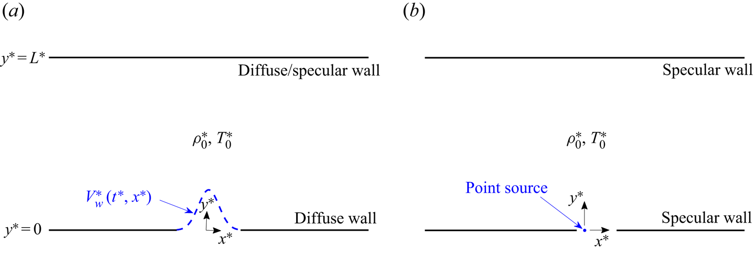
Figure 1. Schematic of the problem: a gas layer, nominally set at thermodynamic equilibrium with uniform density  $\rho _0^*$ and temperature $T_0^*$, is confined in an infinite two-dimensional channel of width $L^*$ with (a) a fully diffuse wall at $y^*=0$ and a fully diffuse or specular boundary at $y^*=L^*$ (‘system A’); (b) fully specular boundaries with a point wall source at the origin (‘system B’). The $y^*=0$ wall (or the origin point source in system B) is actuated with a prescribed small-amplitude time- and $x^*$-dependent normal velocity profile, $V^*_{w}=V^*_{w}(t^*,x^*)$.
The work analyses the effect of gas rarefaction on the two-dimensional propagation of acoustic waves in a channel, generated by the wall excitation profile specified in (2.1). Setting  $L^*$ and $U_{{th}}^*$ as the problem characteristic length scales and velocity scales, respectively, the system response is governed by
 \begin{equation} {Kn}=l^*/L^* , \quad \omega=\omega^*L^*/U_{{th}}^* \quad \mathrm{and} \quad v_{w}(x), \end{equation}
denoting the gas mean Knudsen number and prescribed non-dimensional source oscillation frequency and amplitude, respectively. Here,  $l^*$ marks the mean free path in the gas. The non-dimensional description is completed by taking $\rho _0^*$ and $T_0^*$ as the reference medium density and temperature, respectively, and $\rho _0^*\mathcal {R}^*T_0^*$ as the pressure and stress scale.
In what follows, §§ 3 and 4 analyse the gas response in systems A and B, respectively. In both systems, the specific limits of highly rarefied (collisionless) and continuum conditions are discussed. Collisionless conditions are expected where the channel width  $L^*$ is small compared with $l^*$, i.e. ${Kn}\gg 1$, or where the source frequency $\omega ^*$ is large compared with the mean collision frequency ( $\sim U_{{th}}^*/l^*$), i.e. $\omega {Kn}\gg 1$. Continuum limit conditions should prevail where both ${Kn}\ll 1$ and $\omega {Kn}\ll 1$. The DSMC scheme, applied for counterpart numerical analysis of the problem in system A, is discussed in § 3.3, and is used to validate the limit case approximations and describe the intermediate range of gas rarefaction rates.
3. Diffuse-reflecting wall source
We start by analysing the set-up in figure 1(a), where the  $y=0$ source boundary is diffuse reflecting and the $y=1$ wall is either diffuse or specular reflecting. Limit-case solutions and a discussion of the DSMC numerical scheme are followed by our results for a specific distribution of the wall signal amplitude.
3.1. Free-molecular limit
Focusing on two-dimensional highly rarefied conditions, the gas state is governed by the probability density function  $f=f(t,x,y,\boldsymbol {\xi })$ of finding a gas molecule with velocity about $\boldsymbol {\xi }=(\xi _x,\xi _y,\xi _z)$ at a position near $(x,y)$ at time $t$. At the linearized conditions assumed we express
 \begin{equation} f\left(t,x,y,\boldsymbol{\xi}\right)=F\left[1+\varepsilon\phi\left(t,x,y,\boldsymbol{\xi}\right)\right], \end{equation}
where  $F={\rm \pi} ^{-3/2}\exp [-\xi ^{2}]$ denotes the non-dimensional Maxwellian equilibrium distribution, and $\phi (t,x,y,\boldsymbol {\xi })$ marks the probability perturbation function (Kogan Reference Kogan1969). Assuming the Knudsen number to be large, we consider the collisionless two-dimensional unsteady Boltzmann equation for $\phi (t,x,y,\boldsymbol {\xi })$,
 \begin{equation} \frac{\partial\phi}{\partial t}+\xi_x\frac{\partial\phi}{\partial x}+\xi_y\frac{\partial\phi}{\partial y}=0 . \end{equation}
 Equation (3.2) is subject to a half-range fully diffuse boundary condition at the  $y=0$ oscillating wall, which takes the linearized form
 \begin{equation} \phi(t,x,0,\boldsymbol{\xi}\boldsymbol{{\cdot}}\boldsymbol{\hat{y}}>0)=\rho_{w_+}(t,x)+2\xi_yV_{w}(t,x), \end{equation}
where  $\boldsymbol {\hat {y}}$ is a unit vector directed in the positive $y$-direction (normal to the boundary) and $\rho _{w_+}(t,x)$ is yet unknown. At the $y=1$ boundary, a half-space linearized diffuse or specular condition is imposed,
 \begin{equation} \phi(t,x,1,\boldsymbol{\xi}\boldsymbol{{\cdot}}\boldsymbol{\hat{y}}<0)=\rho_{w_-}(t,x) \quad \mathrm{or} \quad \phi(t,x,1,\boldsymbol{\xi}\boldsymbol{{\cdot}}\boldsymbol{\hat{y}}<0)=\phi(t,x,1,\boldsymbol{\xi}-2(\boldsymbol{\xi}\boldsymbol{{\cdot}}\boldsymbol{\hat{y}})\boldsymbol{\hat{y}}), \end{equation}
respectively, where  $\rho _{w_-}(t,x)$ needs to be determined.
The solution for (3.2) subject to (3.3) and (3.4) with an upper diffuse wall is
 \begin{equation} \phi^{{(diff)}}(t,x,y,\boldsymbol{\xi}) = \left\{ \begin{array}{ll@{}} \rho_{w_-}^{{(diff)}}\left(t-\dfrac{y-1}{\xi _y},x-\dfrac{(y-1)\xi_x}{\xi _y}\right) , & \xi_y< 0,\\ \rho_{w_+}^{{(diff)}}\left(t-\dfrac{y}{\xi_y},x-\dfrac{y\xi_x}{\xi _y}\right)+2\xi_yV_w\left(t-\dfrac{y}{\xi _y},x-\dfrac{y\xi_x}{\xi _y}\right) , & \xi_y>0, \end{array} \right. \end{equation}
whereas for an upper specular boundary
 \begin{align} &\phi^{{(spec)}}(t,x,y,\boldsymbol{\xi}) \nonumber\\ &\quad = \left\{ \begin{array}{@{}ll} \rho_{w_+}^{{(spec)}}\left(t-\dfrac{y-2}{\xi_y},x-\dfrac{(y-2)\xi_x}{\xi _y}\right)-2\xi_yV_w\left(t-\dfrac{y-2}{\xi_y},x-\dfrac{(y-2)\xi_x}{\xi_y}\right) , & \xi_y< 0,\\ \rho_{w_+}^{{(spec)}}\left(t-\dfrac{y}{\xi_y},x-\dfrac{y\xi_x}{\xi _y}\right)+2\xi_yV_w\left(t-\dfrac{y}{\xi _y},x-\dfrac{y\xi_x}{\xi _y}\right) , & \xi_y>0. \end{array} \right. \end{align}
To obtain the wall functions  $\rho _{w_{\pm }}^{{(diff)}}(t,x)$ and $\rho _{w_+}^{{(spec)}}$ appearing in (3.5) and (3.6), we make use of (3.1) and impose the linearized form of the impermeability condition on the $y$-velocity component $v(t,x,y)$ at the walls,
 \begin{equation} v(t,x,0)=\frac{1}{{\rm \pi}^{3/2}}\int_{-\infty}^{\infty}\xi_y\phi(y=0) \mathrm{e}^{-\xi^2}\,\mathrm{d}\boldsymbol{\xi}=V_{w}(t,x) \end{equation}
and
 \begin{equation} v(t,x,1)=\frac{1}{{\rm \pi}^{3/2}}\int_{-\infty}^{\infty}\xi_y\phi(y=1)\mathrm{e}^{-\xi^2}\,\mathrm{d}\boldsymbol{\xi}=0. \end{equation}
The condition at  $y=1$ is trivially satisfied in the case of an upper specular wall. Substituting (3.5) into (3.7), assuming harmonic time dependence of the unknown fields in line with (2.1),
 \begin{equation} \rho_{w_{{\pm}}}^{{(diff)}}(t,x)={Re}\left\{\tilde\rho_{w_{{\pm}}}^{{(diff)}}(x)\exp[\mathrm{i}\omega t]\right\}, \end{equation}
and carrying out the changes of variables  $s=x\pm \xi _x/\xi _y$ in the $\xi _x$-integrals, we obtain a set of coupled integral equations for $\tilde \rho _{w_{\pm }}^{{(diff)}}(x)$,
 \begin{align} &\tilde\rho_{w_+}^{{(diff)}}(x)- \frac{2}{\sqrt{\rm \pi}}\int_{-\infty}^{0}\xi_y^2\exp({-\xi_y^2+\mathrm{i}\omega/\xi_y})\nonumber\\ &\quad\times\int_{-\infty}^{\infty}\exp({-\xi_y^2(s-x)^2})\tilde\rho_{w_-}^{{(diff)}}(s)\,\mathrm{d}s\,\mathrm{d}\xi_y =\sqrt{\rm \pi}v_w(x) \end{align}
and
 \begin{align} &\tilde\rho_{w_-}^{{(diff)}}(x)- \frac{2}{\sqrt{\rm \pi}}\int_{-\infty}^{0}\xi_y^2\exp({-\xi_y^2-\mathrm{i}\omega/\xi_y})\nonumber\\ &\quad\times \int_{-\infty}^{\infty}\exp({-\xi_y^2(s-x)^2})\left[\tilde\rho_{w_+}^{{(diff)}}(s)+2\xi_yv_w(s)\right]\,\mathrm{d}s\,\mathrm{d}\xi_y =0 . \end{align}
Substituting (3.6) into the  $y=0$ condition in (3.7) and following a similar procedure yields an integral equation for $\tilde \rho _{w_{+}}^{{(spec)}}(x)$,
 $$\begin{gather} \tilde\rho_{w_+}^{{(spec)}}(x)- \frac{1}{\sqrt{\rm \pi}}\int_{-\infty}^{0}\xi_y^2\exp({-\xi_y^2+2\mathrm{i}\omega/\xi_y})\nonumber\\ \quad\times \int_{-\infty}^{\infty}\exp({-\xi_y^2(s-x)^2/4})\left[\tilde\rho_{w_+}^{{(spec)}}(s)-2\xi_yv_w(s)\right]\,\mathrm{d}s\,\mathrm{d}\xi_y\nonumber\\ =\sqrt{\rm \pi}v_w(x) . \end{gather}$$
Equations (3.9) and (3.10) are solved numerically via truncation of the infinite-limit integrals at appropriate finite values (where the integrands effectively vanish), discretization along the  $s$-axis and evaluation of the integral terms based on the trapezoidal rule. This yields a system of linear non-homogenous algebraic equations that are solved efficiently using MATLAB. Having obtained $\rho _{w_{\pm }}^{{(diff)}}$ and $\rho _{w_+}^{{(spec)}}$, $\phi ^{{(diff)}}$ and $\phi ^{{(spec)}}$ in (3.5) and (3.6) are known, and appropriate quadratures of (3.1) over the velocity space yield expressions for the $\varepsilon$-scaled hydrodynamic perturbations. Explicit expressions for the density $\rho (t,x,y)$, tangential and normal velocity components, $u(t,x,y)$ and $v(t,x,y)$, respectively, and the normal stress components $P_{xx}(t,x,y)$, $P_{yy}(t,x,y)$ and $P_{zz}(t,x,y)$ are listed in appendix A. Denoting
 \begin{align} &I_{m,n,q}^{({diff})}(x,y)=\frac{1}{\rm \pi} \left\{\frac{1}{(y-1)^m}\int_{-\infty}^0\xi_y^n\exp({-\mathrm{i}\omega(y-1)/\xi_y-\xi_y^2}) \right. \nonumber\\ &\quad \times \int_{-\infty}^{\infty}(x-s)^q\exp({-(x-s)^2\xi_y^2/(y-1)^2})\tilde\rho_{w_-}^{({diff})}(s)\,\mathrm{d}s\,\mathrm{d}\xi_y \nonumber\\ &\quad + \frac{1}{y^m}\int_{0}^{\infty}\xi_y^n\exp({-\mathrm{i}\omega y/\xi_y-\xi_y^2}) \int_{-\infty}^{\infty}(x-s)^q\exp({-(x-s)^2\xi_y^2/y^2})\nonumber\\ &\quad \times \left. \left[\tilde\rho_{w_+}^{({diff})}(s)+2\xi_y v_w(s)\right]\,\mathrm{d}s\,\mathrm{d}\xi_y \right\} \end{align}
and
 \begin{align} &I_{m,n,q}^{({spec})}(x,y)=\frac{1}{\rm \pi} \left\{\frac{1}{(y-2)^m}\int_{-\infty}^0\xi_y^n\exp({-\mathrm{i}\omega(y-2)/\xi_y-\xi_y^2})\right.\nonumber\\ &\quad \times\int_{-\infty}^{\infty}(x-s)^q\exp({-(x-s)^2\xi_y^2/(y-2)^2})\left[\tilde\rho_{w_+}^{({spec})}(s)-2\xi_y v_w(s)\right]\,\mathrm{d}s\,\mathrm{d}\xi_y \nonumber\\ &\quad + \frac{1}{y^m}\int_{0}^{\infty}\xi_y^n\exp({-\mathrm{i}\omega y/\xi_y-\xi_y^2}) \int_{-\infty}^{\infty}(x-s)^q\exp({-(x-s)^2\xi_y^2/y^2})\nonumber\\ &\quad \times\left.\left[\tilde\rho_{w_+}^{({spec})}(s)+2\xi_y v_w(s)\right]\,\mathrm{d}s\,\mathrm{d}\xi_y \right\}, \end{align}
the perturbation-field amplitudes are given by
 \begin{equation} \left. \begin{aligned} \tilde\rho^{({diff})}(x,y) & = I_{1,1,0}^{({diff})} , \quad \tilde u^{({diff})}(x,y)= I_{2,2,1}^{({diff})} , \quad \tilde v^{({diff})}(x,y)= I_{1,2,0}^{({diff})} , \\ \tilde{P}_{xx}^{({diff})}(x,y) & = I_{3,3,2}^{({diff})} , \quad \tilde{P}_{yy}^{({diff})}(x,y)= I_{1,3,0}^{({diff})}, \quad \tilde{P}_{zz}^{({diff})}(x,y)= I_{1,1,0}^{({diff})} /2 \end{aligned} \right\} \end{equation}
in the upper-diffuse-wall case, and
 \begin{equation} \left. \begin{aligned} \tilde\rho^{({spec})}(x,y) & = I_{1,1,0}^{({spec})} , \quad \tilde u^{({spec})}(x,y)= I_{2,2,1}^{({spec})} , \quad \tilde v^{({spec})}(x,y)= I_{1,2,0}^{({spec})} ,\\ \tilde{P}_{xx}^{({spec})}(x,y) & = I_{3,3,2}^{({spec})} , \quad \tilde{P}_{yy}^{({spec})}(x,y)= I_{1,3,0}^{({spec})} , \quad \tilde{P}_{zz}^{({spec})}(x,y)= I_{1,1,0}^{({spec})} /2 \end{aligned} \right\} \end{equation}
in the upper-specular-wall set-up. The time-domain fields are then given by
 \begin{equation} G(t,x,y)={Re}\left\{\tilde{G}(x,y)\exp[\mathrm{i}\omega t]\right\} . \end{equation}
The acoustic pressure  $p(t,x,y)$ is expressed as
 \begin{equation} p(t,x,y)=\frac{2}{3}\left[P_{xx}(t,x,y)+P_{yy}(t,x,y)+P_{zz}(t,x,y)\right] , \end{equation}
and the temperature perturbation may be calculated using the linearized form of the equation of state,  $T(t,x,y)=p(t,x,y)-\rho (t,x,y).$ Our results for the free-molecular system response are presented in § 3.4 for a particular choice of $v_w(x)$.
3.2. Continuum limit
The problem at small Knudsen numbers is next analysed based on a ‘slip flow’ continuum-limit model consisting of the continuum Navier–Stokes–Fourier (NSF) equations and respective wall conditions.
Adopting the scaling introduced in § 2, the linearized two-dimensional NSF equations consist of the balances of mass,
 \begin{equation} \frac{\partial\rho}{\partial t}+\frac{\partial u}{\partial x}+\frac{\partial v}{\partial y}=0 , \end{equation} $x$-momentum,
 \begin{equation} \frac{\partial u}{\partial t}={-}\frac{1}{2}\left(\frac{\partial\rho}{\partial x}+\frac{\partial T}{\partial x}\right)+ \widetilde{{Kn}}\left(\frac{4}{3}\frac{\partial^2 u}{\partial x^2}+ \frac{\partial^2 u}{\partial y^2}+\frac{1}{3}\frac{\partial^2 v}{\partial x\partial y}\right) , \end{equation} $y$-momentum,
 \begin{equation} \frac{\partial v}{\partial t}={-}\frac{1}{2}\left(\frac{\partial\rho}{\partial y}+\frac{\partial T}{\partial y}\right)+ \widetilde{{Kn}}\left(\frac{\partial^2 v}{\partial x^2}+ \frac{4}{3}\frac{\partial^2 v}{\partial y^2}+\frac{1}{3}\frac{\partial^2 u}{\partial x\partial y}\right) \end{equation}
and energy,
 \begin{equation} \frac{\partial T}{\partial t}={-}\frac{\gamma\widetilde{{Kn}}}{{Pr}}\left(\frac{\partial^2 T}{\partial x^2}+\frac{\partial^2 T}{\partial y^2}\right) -(\gamma-1)\left(\frac{\partial u}{\partial x}+\frac{\partial v}{\partial y} \right) , \end{equation}
where the linearized form of the equation of state for an ideal gas,  $p=\rho +T$, has been applied. In (3.18)–(3.19), the viscosity-based Knudsen number,
 \begin{equation} \widetilde{{Kn}}=\frac{\mu_0^*}{\rho_0^*U_{{th}}^*L^{*}}, \end{equation}
is introduced, where  $\mu _0^*$ denotes the gas dynamic viscosity at the reference temperature $T_0^*$. Considering a hard-sphere gas kinetic model, $\mu _0^*=(\eta \sqrt {{\rm \pi} }/4)\rho _0^*U_{{th}}^*l^*$ with $\eta \approx 1.27$ (Sone Reference Sone2007), yielding $\widetilde {{Kn}}=(\eta \sqrt {{\rm \pi} }/4){Kn}$ (cf. (2.2a–c)). Also appearing in (3.19) are the gas Prandtl number, ${Pr}$, and the ratio of specific heats, $\gamma$, which equal $2/3$ and 5/3, respectively, for an ideal monatomic gas. (3.16)–(3.19) are supplemented by the wall impermeability conditions,
 \begin{equation} v(t,x,0)=V_w(t,x) \quad \mathrm{and} \quad v(t,x,1)=0, \end{equation}
together with first-order velocity slip,
 \begin{equation} u(t,x,0)=c_u\left(\frac{\partial u}{\partial y}+\frac{\partial v}{\partial x}\right)_{(t,x,0)}+c_T^{(1)}\left.\frac{\partial T}{\partial x}\right|_{(t,x,0)} \end{equation}
and
 \begin{equation} u(t,x,1)=c_u\left(-\frac{\partial u}{\partial y}+\frac{\partial v}{\partial x}\right)_{(t,x,1)}+c_T^{(1)}\left.\frac{\partial T}{\partial x}\right|_{(t,x,1)}, \end{equation}
and temperature jump,
 \begin{equation} T(t,x,0)=c_T^{(2)}\left.\frac{\partial T}{\partial y}\right|_{(t,x,0)} \quad \mathrm{and} \quad T(t,x,1)={-}c_T^{(2)}\left.\frac{\partial T}{\partial y}\right|_{(t,x,1)}, \end{equation}
conditions, as formulated by Aoki et al. (Reference Aoki, Baranger, Hattori, Kosuge, Martalo, Mathiaud and Mieussens2017a). Conditions (3.22) and (3.23a,b) are valid for fully diffuse boundaries only, whereas the realization of specular walls at  ${Kn}\rightarrow 0$ will be considered in § 4. A temperature jump component contributed by the normal stress at the wall ( $\propto \partial v/\partial y$) is not included in (3.23a,b), as it is of higher-order in the present linearized set-up (cf. Eq. (118) in Aoki et al. (Reference Aoki, Baranger, Hattori, Kosuge, Martalo, Mathiaud and Mieussens2017a) et seq.). We have numerically validated that inclusion of this term has no visible effect on the results obtained. Strictly, the boundary conditions analysis by Aoki et al. (Reference Aoki, Baranger, Hattori, Kosuge, Martalo, Mathiaud and Mieussens2017a) is restricted to a rigid body motion of the surface. Yet, in the present linearized and time-harmonic set-up, the amplitude of boundary motion is taken arbitrarily small about its nominal location, so that any physical displacement of the wall is negligible. This is equivalent to imposing the impermeability condition on a stationary boundary position with prescribed small-amplitude normal velocity. Assuming a hard-sphere gas model,
 \begin{equation} c_u\approx1.111{Kn} , \quad c_T^{(1)}\approx0.573{Kn} \quad \mathrm{and} \quad c_T^{(2)}\approx2.127{Kn} , \end{equation}
where the above numerical values have been obtained after multiplying their counterparts in Aoki et al. (Reference Aoki, Baranger, Hattori, Kosuge, Martalo, Mathiaud and Mieussens2017a) by  $\sqrt {{\rm \pi} }/2$ due to different scaling.
Considering sinusoidal time dependence of all fields as in (3.14) and applying the  $x$-Fourier transform,
 \begin{equation} \bar{G}(k,y)=\int_{-\infty}^{\infty}\tilde{G}(x,y)\exp[-\mathrm{i}kx]\,\mathrm{d} x, \end{equation}
the system of (3.16)–(3.19) is transformed into
 \begin{equation} \left. \begin{gathered} \mathrm{i}\omega\bar\rho+\mathrm{i}k\bar{u}+\bar{v}'=0 , \quad \mathrm{i}\omega\bar u={-}\frac{\mathrm{i}k}{2}\left(\bar\rho+\bar T\right)+ \frac{\eta{Kn}\sqrt{\rm \pi}}{4}\left(\bar u''-\frac{4k^2}{3}\bar{u}+ \frac{\mathrm{i}k}{3}\bar v'\right) ,\\ \mathrm{i}\omega\bar v={-}\frac{1}{2}\left(\bar\rho'+\bar T'\right)+ \frac{\eta{Kn}\sqrt{\rm \pi}}{4}\left(\frac{\mathrm{i}k}{3}\bar u'+\frac{4}{3}\bar{v}''-k^2\bar v\right)\\ \mathrm{and} \quad \mathrm{i}\omega \bar T={-}\frac{5\eta{Kn}\sqrt{\rm \pi}}{8}\left(\bar T''-k^2\bar T\right) -\frac{2}{3}\left(\mathrm{i}k \bar u+\bar v' \right) , \end{gathered} \right\} \end{equation}
where primes denote derivatives in the  $y$-direction. These are supplemented by the transformed form of the boundary conditions in (3.21)–(3.23),
 \begin{equation} \left. \begin{gathered} \bar v(k,0)=\bar v_w(k) , \quad \bar v(k,1)=0,\\ \bar u(k,0)=\left[c_u\left(\bar u'+\mathrm{i}k\bar v\right)+\mathrm{i}kc_T^{(1)}\bar T\right]_{(k,0)} \ , \ \bar u(k,1)=\left[c_u\left(-\bar u'+\mathrm{i}k\bar v\right)+\mathrm{i}kc_T^{(1)}\bar T\right]_{(k,1)},\\ \bar T(k,0)=c_T^{(2)}\bar T'{(k,0)} \quad \mathrm{and} \quad \bar T(k,1)={-}c_T^{(2)}\bar T'{(k,1)}. \end{gathered} \right\} \end{equation}
 To analyse the problem in (3.26)–(3.27), the transformed density  $\bar \rho (k,y)$ is extracted from the continuity equation in (3.26),
 \begin{equation} \bar\rho={-}\frac{k}{\omega}\bar{u}+\frac{\mathrm{i}}{\omega}\bar{v}', \end{equation}
and substituted into the  $x$- and $y$-momentum balances. The system obtained is cast as a set of six coupled first-order equations,
 \begin{equation} \boldsymbol{g}'=\boldsymbol{\mathsf{A}}\boldsymbol{g}, \end{equation}
where  $\boldsymbol {g}=[\bar u, \bar u' ,\bar v,\bar v',\bar T,\bar T']^{\textrm {T}}$ is the vector of unknown functions and $\boldsymbol{\mathsf{A}}=\boldsymbol{\mathsf{A}}(k,{{Kn}})$ is the matrix of coefficients. The general solution for (3.29) is
 \begin{equation} \boldsymbol{g}=\varSigma_{n=1}^{6} D_n\boldsymbol{v_n}\exp[\beta_ny], \end{equation}
where  $\boldsymbol {v_n}(k,{Kn},\omega )$ and $\beta _n(k,{{Kn}},\omega )$ mark the $n=1,\ldots,6$ eigenvectors and eigenvalues of the matrix $\boldsymbol{\mathsf{A}}$, respectively, and $D_n$ are unknown scalar coefficients to be determined using the walls boundary conditions. Analysis of the characteristic sixth-order polynomial of the matrix $\boldsymbol{\mathsf{A}}$ at ${Kn}\ll 1$ indicates that its roots $\beta _n$ consist of three complex pairs of alternating signs. Carrying a ${Kn}\ll 1$ expansion of the characteristic equation, approximate expressions for $\beta _n(k,{{Kn}},\omega )$ are obtained,
 \begin{equation} \left. \begin{gathered} \beta_{1,2}={\pm}\mathrm{i}\sqrt{\frac{6\omega^2-5k^2}{5}}\left[1-\frac{21\mathrm{i}\eta\sqrt{\rm \pi}\omega^3}{10(6\omega^2-5k^2)}{Kn}+O\left({Kn}^2\right)\right],\\ \beta_{3,4}={\pm}\frac{2\sqrt{\mathrm{i\omega}}}{\sqrt{{\rm \pi}^{1/2}\eta{Kn}}}\left[1+O\left({Kn}\right)\right] \quad \mathrm{and} \quad \beta_{5,6}={\pm}\frac{2\sqrt{2\mathrm{i}\omega}}{\sqrt{3{\rm \pi}^{1/2}\eta{Kn}}}\left[1+O\left({Kn}\right)\right]. \end{gathered} \right\} \end{equation}
As  ${Kn}\rightarrow 0$, $\beta _{1,2}$ converge to their ideal-flow limit, $\mathrm {i}\beta =\pm \sqrt {(6\omega ^2-5k^2)/5}$, effective at inviscid compressible flow conditions (see (4.10)–(4.12)). The $\beta _{3,4}$ and $\beta _{5,6}$ eigenvalues, as well as the $O({Kn})$ correction for $\beta _{1,2}$, reflect viscous and heat conduction effects, inevitably missing at Euler-flow conditions.
To specify the particular solution in (3.30), the coefficients  $D_{n}$ multiplying $\boldsymbol {v_{n}}\exp [\beta _{n}y]$ are calculated via the imposition of the impermeability, slip and jump wall conditions in (3.27). The result in the physical $(t,x,y)$ plane is then obtained by applying the inverse transform,
 \begin{equation} G(t,x,y)=\frac{1}{2{\rm \pi}}{Re}\left\{\exp[\mathrm{i}\omega t]\int_{-\infty}^{\infty}\bar{G}(k,y)\exp\left[\mathrm{i}kx\right]\,\mathrm{d}k\right\} , \end{equation}
to each of the hydrodynamic perturbations.
3.3. Numerical scheme: DSMC method
The DSMC method, initially proposed by Bird (Bird Reference Bird1994), is a stochastic particle method commonly applied for the analysis of rarefied gas flows. In the present work, we make use of the DSMC scheme to examine the free-molecular and continuum limit solutions derived in §§ 3.1 and 3.2, respectively, and to capture the system behaviour at intermediate Knudsen numbers. We accordingly adopt Bird's algorithm, together with the hard-sphere model of molecular interaction, to simulate the gas state. In line with the problem formulation, the wall at  $y^*=0$ is assumed fully diffuse with a prescribed $x^{*}$-dependent time-harmonic normal velocity profile. The stationary wall at $y^*=L^*$ is taken either fully diffuse or specular. A fixed temperature $T_0^*$ is assigned at the diffuse surfaces.
In a recent contribution (Manela & Ben-Ami Reference Manela and Ben-Ami2021), the authors have developed an algorithm for simulating small-amplitude non-uniform wall normal velocity conditions, while maintaining the surface fixed. This has been achieved by adding or subtracting particles and ensuring that the number flux of gas particles emitted at the boundary agrees with the flux required to satisfy the impermeability condition. The same algorithm is applied in the present work to simulate the vibroacoustic signal at the wall  $y^*=0$, specified in (2.1). Additionally, the present simulation also calculates the normal acoustic force acting at the stationary $y^*=L^*$ boundary. This is carried out via summation over the change in the $y^*$-momentum of all $i=1,\ldots,N$ particles reflected at the $y^*=L^*$ stationary surface during a time interval $[t^*,t^*+\Delta t^*]$,
 \begin{equation} F^{*}_{s}(t^*) = \frac{m^*}{\Delta t^*}\sum_{i=1}^N \left(\xi_{y,i}^{{in}*}-\xi_{y,i}^{{out}*}\right). \end{equation}
Here,  $m^*$ marks the gas molecular mass, and the superscripts ‘ $in$’ and ‘ $out$’ correspond to the respective properties of incoming and reflected particles.
In each simulation, the computation has started from an initial equilibrium state and followed in time through a final periodic state, typically established after two to three oscillation periods. To mimic the formulated infinite channel set-up (yet maintain a finite computation domain), virtual ‘side’ boundaries have been placed sufficiently far from the source zone to not affect the system response. Since the signal decay rate decreases with decreased rarefaction, this has required simulating larger channel sections, and resulted in demanding computations at continuum-limit conditions. In a typical calculation, the domain was divided into  $4- 12\times 10^{3}$ equally sized cells. An additional division of each cell into collisional subcells was carried out to comply with the mean-free-path limitations. The subcells’ size was set to a maximum of $l^{*}/4$, and the simulation time step was taken as $0.25/U_{{th}}^{*} \times \min \{ l^{*},\Delta x^*, \Delta y^* \}$, where $\Delta x^*$ and $\Delta y^*$ are the cell dimensions. A typical run consisted of $\approx 4\times 10^7$ particles and was followed for three to four periods, where the results presented were taken from the last period. To sufficiently reduce the statistical noise inherent in DSMC calculations, the results were averaged over a large number of realizations of the above procedure. The number of samples taken was $\approx 500$ in the ballistic limit and only $\approx 50$ in the continuum limit ( ${Kn}=0.01$), where DSMC computations become extremely time consuming. This may be viewed by the much larger noise-to-signal ratio obtained in the simulation results in figure 4 compared with figure 2. Since the wall signal considered below (see (3.34)) is symmetric about $x=0$, the expected flow field symmetry was applied to average over the simulation output in the $x<0$ and the $x>0$ plane parts, as a means for further reducing numerical noise scatter. Each simulation lasted from several hours in the free-molecular limit up to a week in the continuum limit using a 10-core Intel i7-6950 machine. In line with the linearized problem formulation, a value of $\varepsilon =0.04$ was taken, for which nonlinear effects were found negligible.
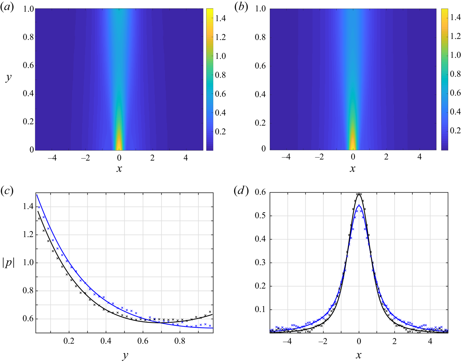
Figure 2. Effect of the scattering wall condition on the free-molecular acoustic pressure amplitude at  $\omega =1$: (a,b) colourmaps of the pressure amplitude for a scattering $y=1$ diffuse (a) and specular (b) wall systems; (c,d) sections of the acoustic pressure amplitude at (c) $x=0$ and (d) $y=0.85$. The black and blue curves in (c,d) correspond to channels with $y=1$ diffuse and specular boundaries, respectively, and the crosses show respective DSMC predictions at ${Kn}=5$. All the results are for Gaussian wall excitation with $\alpha =10$.
3.4. Results
To illustrate our findings, we present results for a Gaussian-distributed wall signal source amplitude,
 \begin{equation} v_w^{(G)}(x)=\exp\left[-\alpha x^2\right], \end{equation}
where  $\alpha$ is a fixed constant, taken sufficiently large ( $\alpha =10$) to focus on a relatively ‘localized’ excitation. For practical purposes, the Gaussian distribution aims at resembling a two-dimensional counterpart of a vibrating membrane. A similar configuration has been depicted by the acoustic resonators geometries shown in figure 5 in Abdolvand et al. (Reference Abdolvand, Bahreyni, Lee and Nabki2016), also sketched in figure 1 of Lu & Horsley (Reference Lu and Horsley2015) and in the vibroacoustic measurements of Julius et al. (Reference Julius, Gold, Kleiman, Leizeronok and Cukurel2018) (see figure 4 therein). The analytical limit-case results are compared with DSMC predictions for the purposes of numerical validation and illustration of the system behaviour at intermediate flow conditions. The results in the continuum-limit regime follow the procedure outlined in § 3.2 with $\bar {v}_w^{(G)}(k)=\sqrt {{\rm \pi} /\alpha }\exp [-k^2/4\alpha ]$. The inverse Fourier transform, as well as the quadratures required in the free-molecular solution in § 3.1, are calculated numerically.
3.4.1. The acoustic flow field
Starting with the free-molecular regime, figure 2 presents the effect of the  $y=1$ scattering wall condition (diffuse or specular) on the ${Kn}\rightarrow \infty$ acoustic pressure amplitude at $\omega =1$. Figure 2(a,b) show colourmaps of the pressure amplitude with a scattering diffuse or specular wall, respectively, whereas figure 2(c,d) present detailed comparisons with DSMC ${Kn}=5$ predictions of the diffuse- and specular-wall signals at $x=0$ and $y=0.85$, respectively. At first we note the general minor differences between the diffuse and specular wall systems, where both signals are confined to the proximity of the source zone and mainly propagate to the scattering wall in the normal $y$-direction. While the colourmaps in figure 2(a,b) appear nearly identical, slight differences are viewed in figure 2(c,d), where the specular-wall signal (marked by the blue curves) penetrates to a slightly larger distance from the source (see figure 2d). Indeed, since no energy is absorbed by the $y=1$ surface in the specular-wall case, the respective pressure fluctuation spreads over a larger $x$-distance in the spanwise direction. The close agreement in figure 2(c,d) between the free-molecular and DSMC predictions at ${Kn}=5$ supports these findings. The simulation results in the ballistic limit (not presented here) do not exhibit any visible differences from the ${Kn}=5$ data. The free-molecular solution has the advantage of producing smoothly varying results with minimal computational effort, whereas the inherent numerical noise contained in the DSMC signal is clearly visible. Since practically negligible differences have been obtained between the diffuse- and specular-wall systems, further results will focus on a diffuse walls system only.
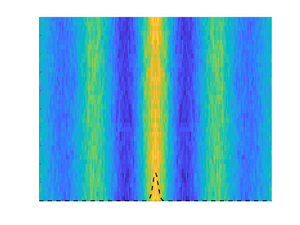
Maintaining  $\omega =1$, figure 3 presents the effect of gas rarefaction on the acoustic pressure signal. To this end, the figure shows time snapshots, at period time $(t=2{\rm \pi} /\omega$), of the acoustic disturbance at a sequence of Knudsen numbers varying between the free-molecular ( ${Kn}\rightarrow \infty$, figure 3a) and near-continuum ( ${Kn}=0.05$, figure 3f) regimes. The ${Kn}\rightarrow \infty$ field in figure 3(a) is obtained using the analysis in § 3.1, while figure 3(b–f) present DSMC predictions. The statistical noise inherent in the DSMC-calculated signals is noted again. As stated in § 3.3, DSMC computations become significantly demanding with decreasing ${Kn}$, due to both the increased number of molecular collisions and the required extension in the computation domain, to prevent unwarranted reflections from the far virtual sidewalls.

Figure 3. Variation with  ${Kn}$ of the acoustic pressure at period time ( $t=2{\rm \pi} /\omega$) in response to Gaussian wall excitation with $\alpha =10$ and $\omega =1$ in a channel with diffuse walls: (a) ${Kn}\rightarrow \infty$; (b) ${Kn}=5$; (c) ${Kn}=1$; (d) ${Kn}=0.5$; (e) ${Kn}=0.1$; (f) ${Kn}=0.05$. The results in (a) are based on the free-molecular analysis and the colourmaps in (b–f) show DSMC predictions.
Comparing between the results in figure 3(a–c), it is seen that free-molecular conditions essentially prevail through  ${Kn}\gtrsim 1$, as also supported by the comparisons in figure 2(c,d) at ${Kn}=5$. Yet, with further decreasing ${Kn}$, a decaying wave-like pattern of the signal in the $\pm x$-directions is observed, characterized by a unique wavenumber. The decay rate decreases with decreasing ${Kn}$, hence the acoustic perturbation propagates to larger $|x|$-distances. Notably, the pressure field varies mainly in the $x$-direction, while markedly weak $y$-dependence is seen at near-continuum conditions. As will be discussed in § 4, in the ideal-flow ( ${Kn}\rightarrow 0$) regime, the above behaviour degenerates to the propagation of a non-decaying one-dimensional acoustic wave at a wavelength of $\lambda =2{\rm \pi} \sqrt {5/6}/\omega$.
To further inspect the system behaviour in the continuum limit, figure 4 compares between DSMC and NSF predicted pressure fields at  ${Kn}=0.01$ and $\omega =1$. Figure 4(a,b) show period-time snapshots of the DSMC- and NSF-calculated fields, which, at first, appear rather different. The observed discrepancies originate from errors introduced by both schemes. In the DSMC computation, spurious reflections from the side virtual walls (placed at $x=\pm 15$ for ${Kn}=0.01$) affect the pressure field. In the NSF model, the acoustic boundary layers (of width $\sim O(\sqrt {{Kn}})\sim 0.1$, see Inaba et al. (Reference Inaba, Yano and Watanabe2012) and Hattori & Takata (Reference Hattori and Takata2019)) occurring along the channel walls, as well as the regions in the vicinity of the source and its $y=1$ reflection, are not captured well. Indeed, within the neighbourhood of the localized wall excitation, the local Knudsen number, based on the characteristic length scale of the wall velocity profile (see (3.34)), becomes significantly larger, resulting in the breakdown of the continuum-limit description. The above discrepancies are highlighted in figure 4(d), comparing between the NSF- and DSMC-calculated signals at $y=0.1$ and $t=2{\rm \pi} /\omega$. The effect of the high local Knudsen number is viewed through the large deviation between the fields about $x=0$, whereas the discrepancies at large $|x|\gtrsim 5$ may be attributed to the DSMC-calculated reflections from the sidewalls. After partially removing these zones from figure 4(b), the zoomed-in pressure field at the channel bulk in figure 4(c) closely agrees with the DSMC-calculated field in figure 4(a). With decreasing ${Kn}$, the unwarranted inaccuracies of the continuum-limit model should diminish, and the slip-flow solution is expected to accurately capture the entire system behaviour. Due to the costly DSMC calculations required for ${Kn}<0.01$ simulations, a comparison at lower Knudsen numbers was not carried out for further verification. Similarly, examination of the comparison for Gaussian excitations with lower $\alpha$ (where near-source gradients are smaller) is precluded, since the signal propagates to larger distances with decreasing $\alpha$, necessitating the modelling of a larger computational domain, which is not in the capacity of our computational resources. A better approximation of the near-field source zone at small (yet finite) Knudsen numbers may be achieved using high-order hydrodynamic models, such as extended moment schemes (Struchtrup Reference Struchtrup2005). The application of these models, however, is not in the scope of the present contribution.

Figure 4. Comparison between  ${Kn}=0.01$ NSF slip flow and DSMC predicted acoustic pressure fields at period time ( $t=2{\rm \pi} /\omega$) in response to Gaussian wall excitation with $\alpha =10$ and $\omega =1$ in a channel with diffuse walls: (a,b) colourmaps of the (a) DSMC and (b) NSF-calculated pressures; (c) zoom-in of the NSF field within the strip confined by the dashed lines in (b); (d) $x$-variations of the NSF (solid curve) and DSMC (crosses) fields at $y=0.1$. The dark-blue zones in (b) mark regions in the vicinity of the source origin and $y=1$ facing reflection removed from the presentation for better clarity (see discussion).
Figure 5 examines the effect of the signal time-frequency  $\omega$ on the free-molecular (figure 5a,b) and continuum-limit ( ${Kn}=0.004$, figure 5c,d) system response. The figure presents $x$-distributions at $y=0.5$ of the pressure amplitude (figure 5a,c) and time snapshots at period time (figure 5b,d) in response to source actuation at $\omega =0.2,1$ and $5$. A comparison is made between the free-molecular and DSMC predictions at ${Kn}=5$, supporting the occurrence of collisionless flow conditions at the indicated ${Kn}$ and the presented frequencies.

Figure 5. Effect of the signal time-frequency  $\omega$ on the (a,b) free-molecular ( ${Kn}\rightarrow \infty$) and (c,d) slip flow NSF ( ${Kn}=0.004$) acoustic pressure: $x$-distributions at $y=0.5$ of the pressure amplitude (a,c) and time snapshots at period time ( $t=2{\rm \pi} /\omega$, panels b,d). The numbers indicate the values of $\omega$. All results are for Gaussian wall excitation with $\alpha =10$ and a channel with fully diffuse walls. The crosses in panels (a,b) show DSMC predictions at ${Kn}=5$.
Considering the free-molecular fields in figure 5(a,b), we observe that the signal extends over larger distances from the source with decreasing  $\omega$, and maintains higher pressure amplitudes. In contrast, at large frequencies the acoustic fluctuations are confined to the proximity of the source, and the effect of the channel $y=1$ wall becomes negligible. This is a consequence of our numerical solution for (3.9), indicating that the integral terms therein are negligibly small at $\omega \gg 1$, yielding
 \begin{equation} \tilde\rho^{{(diff)}}_{w_+}(x;\omega\gg1)\approx\sqrt{\rm \pi}v_w(x) \quad \mathrm{and} \quad \tilde\rho^{{(diff)}}_{w_-}(x;\omega\gg1)\ll1. \end{equation}
(The large- $\omega$ decay rate of $\tilde \rho ^{{(diff)}}_{w_-}(x)$ may be evaluated by substituting $\tilde \rho ^{{(diff)}}_{w_+}=\sqrt {{\rm \pi} }v_w(x)$ into the second equation in (3.9) and taking the $\omega \gg 1$ limit, yet the details are skipped here for brevity.) The problem at $\omega \gg 1$ therefore degenerates into its semi-infinite counterpart, considered in Manela & Ben-Ami (Reference Manela and Ben-Ami2021). At lower $\omega \sim O(1)$ values, the signal decay rate reduces, and the effect of the stationary wall reflections, intensifying the transmission of sound to larger $x$-distances, becomes significant. While a general reduction in pressure amplitude with increasing $\omega$ is also observed in the continuum limit, the results in figure 5(c,d) show a qualitatively different behaviour compared with the free-molecular regime. Here, the acoustic pressure is oscillatory decaying with $x$, exhibiting fluctuations that are characterized by a shorter wavelength at higher frequencies. In figures 3(e–f) and 4(a–c), these fluctuations are reflected as the decaying $x$-wise wave patterns of the acoustic signal (see also figure 9 et seq.).
3.4.2. The acoustic force on the walls
As mentioned in the introduction, a key parameter in the design and operation of microsize oscillators is the force generated by the gas layer on the apparatus walls. In the current set-up, the gas loadings per unit length normal to the vibrating and stationary boundaries, scaled by  $\rho _0^*\mathcal {R^*}T_0^*L^*$, are
 \begin{equation} F_{v}(t;{Kn},\omega)=\int_{-\infty}^{\infty}P_{yy}(t,x,0)\,\mathrm{d} x \quad \mathrm{and} \quad F_{s}(t;{Kn},\omega)=\int_{-\infty}^{\infty}P_{yy}(t,x,1)\,\mathrm{d} x, \end{equation}
respectively, while the tangential forces vanish due to problem symmetry. Following the above analysis,  $F_{v}(t)$ and $F_{s}(t)$ may be evaluated in both collisionless and continuum limits. Considering the former and focusing on the upper-diffuse-wall system, we substitute $\tilde P_{yy}^{({diff})}(x,y)$ in (3.12) together with (3.14) into (3.36a,b), to obtain
 \begin{equation} \left. \begin{aligned} & F_{v}(t;{Kn}\gg1,\omega)=2\mathrm{e}^{\mathrm{i}\omega t} \int_{-\infty}^{\infty}\left[\frac{\tilde\rho_{w_+}(x)}{4} + \frac{v_w(x)}{\sqrt{\rm \pi}} -\frac{1}{\rm \pi}\int_{-\infty}^0\xi_y^3\exp\left({-\xi_y^2+\frac{\mathrm{i}\omega}{\xi_y}}\right)\right.\\ & \quad \times \left. \int_{-\infty}^{\infty} \exp({-\xi_y^2(s-x)^2})\tilde\rho_{w_-}(s)\,\mathrm{d}s\,\mathrm{d}\xi_y \right]\,\mathrm{d} x, \\ & F_{s}(t;{Kn}\gg1,\omega)=2\mathrm{e}^{\mathrm{i}\omega t} \int_{-\infty}^{\infty}\left[\frac{\tilde\rho_{w_-}(x)}{4} + \frac{1}{\rm \pi}\int_0^{\infty}\xi_y^3\exp\left({-\xi_y^2-\frac{\mathrm{i}\omega}{\xi_y}}\right)\right.\\ & \quad \times\left.\int_{-\infty}^{\infty} \exp\left({-\xi_y^2(s-x)^2}\right)\left(\tilde\rho_{w_+}(s)+2\xi_yv_w(s)\right)\,\mathrm{d}s\,\mathrm{d}\xi_y \right]\,\mathrm{d} x . \end{aligned} \right\} \end{equation}
Substituting the continuum-limit expression for  $P_{yy}$ into (3.36a,b) and applying the analysis in § 3.2, we obtain
 \begin{equation} F_{v,s}(t;{Kn}\ll1,\omega)=\frac{\mathrm{e}^{\mathrm{i}\omega t}}{2{\rm \pi}} \int_{-\infty}^{\infty}\int_{-\infty}^{\infty} \left[-\bar p+\frac{5\sqrt{\rm \pi}}{12}{Kn}\left(2\bar v'-\mathrm{i}k\bar u\right)\right]_{y=\{0,1\}} \mathrm{e}^{\mathrm{i}kx} \,\mathrm{d}k\,\mathrm{d} x. \end{equation}
Here, our numerical calculations indicate that the contribution of the  $O({Kn})$ viscous-stress term (vanishing at ideal-flow conditions) is small.
Figure 6 presents the variation with  $\omega /{\rm \pi}$ of the amplitudes of the normal forces on the vibrating (figure 6a) and stationary (figure 6b) walls. Each figure part compares between the free-molecular ( ${Kn}\rightarrow \infty$) and continuum-limit ( ${Kn}=0.004$ and ${Kn}=0.001$) results. The blue circles in figure 6(b) mark DSMC-calculated predictions at ${Kn}=5$ for $|F_s|$, showing close agreement with the respective free-molecular values. The divergence of the force at low frequencies ( $\omega \rightarrow 0$) in all cases should be accounted as a non-physical effect of our model, since the associated $O(\varepsilon /\omega )$ wall displacement (see (2.1)) cannot be considered small, thus violating the linearized scheme assumption.

Figure 6. Variations with  $\omega /{\rm \pi}$ of the amplitudes of the normal forces on the $y=0$ (a) and $y=1$ (b) walls: comparison between continuum-limit ( ${Kn}=0.004$ and $0.001$, black and red lines, respectively) and free-molecular ( ${Kn}\rightarrow \infty$, blue curves) predictions. The blue circles in (b) present DSMC data at ${Kn}=5$. The results are for a fully diffuse channel with Gaussian wall excitation at $\alpha =10$.
Focusing on continuum-limit conditions in figure 6(a,b), we observe that the walls’ forces exhibit distinct descending peaks at  $\omega$ values approaching
 \begin{equation} \omega_n\approx n{\rm \pi}\sqrt{{5}/{6}} , \quad n=1,2,\ldots \end{equation}
as  ${Kn}\rightarrow 0$. The $\sqrt {{5}/{6}}$ factor appearing in (3.39) originates from the scaling introduced in § 2, in which the frequency has been normalized by $U_{{th}}^*/L^*$, rather than by the continuum speed-of-sound-based $c_0^*/L^*$ measure (where $c_0^*=\sqrt {\gamma \mathcal {R}^*T_0^*}$). The resonance frequencies noted in (3.39) correspond to the acoustic wavelengths
 \begin{equation} \lambda_n =2{\rm \pi}/\omega_n\approx 2\sqrt{{6}/{5}}/n , \quad n=1,2,\ldots, \end{equation}
indicating that large force amplitudes at continuum-limit conditions occur in cases where the channel width is in the proximity of the acoustic wave antinodes. In contrast, effective minima in the acoustic force take place in set-ups where the generated acoustic wave has its node points at the channel walls, i.e. for
 \begin{equation} \omega_{n/2}={\rm \pi}(n+1/2)\sqrt{{5}/{6}} \quad\mathrm{and} \quad \lambda_{n/2}=4\sqrt{{6}/{5}}/(2n+1) , \quad n=0,1,\ldots \end{equation}
Since non-ideal flow conditions prevail in all cases (where the Knudsen number is small yet finite), viscous effects are present to some extent, causing the damping of the resonance- and antiresonance-like system behaviour. The force maxima reduce with increasing  $\omega _n$ (and decreasing $\lambda _n$), due to the growing impact of viscous dissipation on shorter waves.
In qualitative difference from the continuum-limit response, the acoustic forces in the free-molecular regime do not exhibit any resonance-like frequency dependence. Here, as viewed by the results in figures 2, 3(a) and 5(a,b), the  $(x,y)$ flow pattern is not governed by a single dominant wave, as the continuum wave equation model is not followed. Inspecting the blue curve in figure 6(b), we find that the force amplitude at the $y=1$ wall decreases nearly monotonically and approaches a vanishing value at large $\omega$. The force at the $y=0$ surface shows non-monotonic variation between ${\rm \pi} /2\lesssim \omega \lesssim {\rm \pi}$ and reaches a constant value at large $\omega$. Indeed, in the $\omega \gg 1$ limit, substituting (3.35a,b) together with the Gaussian signal considered in (3.34) into (3.37), we find
 \begin{equation} F_{v}^{(G)}(t;{Kn}\gg1,\omega\gg1)\approx\frac{{\rm \pi}+4}{2\sqrt{\alpha}} \, \mathrm{e}^{\mathrm{i}\omega t}, \end{equation}
while  $F_{s}(t;{Kn}\gg 1,\omega \gg 1)$ is asymptotically small. Equation (3.42) captures the $\omega \gg 1$ limit of $|F_{v}|\approx 1.13$ shown by the blue line in figure 6(a) for $\alpha =10$.
Summarizing the results in figure 6, the free-molecular acoustic force on the vibrating wall retains a nearly constant value at  $\omega \gtrsim {\rm \pi}$, where it is governed primarily by its ‘near-field’ interaction with the gas, and is nearly unaffected by channel confinement. The situation markedly changes at the $y=1$ boundary: here, the monotonic decay of $|F_{s}|$ occurs due to the reduced interaction of the acoustic signal with the far wall. While a quantitative comparison between the non-dimensional free-molecular and continuum-limit force amplitudes is obviated due to the different scaling introduced (each normalized by $\rho _0^*\mathcal {R^*}T_0^*L^*$), it is worthwhile noting that the free-molecular force (valid also at large yet finite ${Kn}$) becomes larger than its continuum-limit counterpart close to the continuum-based $\omega _{n/2}={\rm \pi} (n+1/2)\sqrt {{5}/{6}}$ ( $n=0,1,\ldots$) nodes at $y=0$, and near the respective $n=0$ node at $y=1$. This result should remain inevitably effective also in dimensional quantities for systems at sufficiently small Knudsen numbers, due to their antiresonance behaviour resulting in a vanishingly small force (cf. figure 10).
4. Point wall source in a specular-reflecting channel
The set-up illustrated in figure 1(b), containing a specular-reflecting channel with a point delta source located at its  $y=0$ boundary,
 \begin{equation} v_w^{(\delta)}(x)=\delta(x), \end{equation}
is next considered. Here, the effect of the channel upper wall scattering may be analytically expressed in terms of the semi-infinite solution presented in Manela & Ben-Ami (Reference Manela and Ben-Ami2021), and its superposition with appropriate images about the channel surfaces. This simplifies the description of the effect of upper-wall confinement, in terms of both mathematical and physical rationalizations. The analysis is carried out in the free-molecular and ideal-flow limits. DSMC calculations were not carried out due to the ambiguous representation of a delta-function source in the simulation. Recalling the results in the previous section, indicating a minor quantitative effect of the scattering wall condition (being fully diffuse or specular) on the acoustic field properties, the following analysis aims at further shedding light on the general impact of channel confinement on sound propagation at non-continuum conditions. To relate to the Gaussian wall distribution studied above, the  $\alpha \gg 1$ limit of $v_w(x)=\sqrt {\alpha /{\rm \pi} }\exp [-\alpha x^2]$ distribution yields the present delta function. Advantageously, its relative simplicity enables the derivation of the closed-form results presented below. Being a limit case of an ‘infinitely steep’ Gaussian, it is expected that the delta function system reflects qualitatively similar results to the Gaussian case, yet with larger amplitudes and gradients in the vicinity of the point source, as illustrated subsequently.
4.1. Free-molecular limit
As the effect of molecular collisions is negligible in this limit and all particle–surface interactions are taken specular, any disturbance in gas equilibrium occurs directly due to particles emission from the point source. Specifically, such particles may arrive at an  $(x_0,y_0)$ channel bulk location either via ‘free flight’ from the source location, or after being reflected by the specular walls in-between source emission and $(x_0,y_0)$ arrival. These scenarios are illustrated schematically in figure 7, where the solid black line marks the free-flight particle path, and the dashed blue and red lines denote trajectories of particles reflected from the source and colliding with the specular channel surfaces once or twice, respectively. Clearly, the dashed colourline trajectories demonstrate the scattering effect of the $y=1$ wall, missing in the half-space problem. Due to the specular-wall interaction considered, this effect may be equivalently modelled as a series of image reflections about the $y=0$ and $y=1$ surfaces, as partially shown by the solid blue ( $y=2$) and red ( $y=-2$) lines in figure 7. The series of wall images (further extending to $y_{{image}}=\pm 2s, s=1,2,\ldots )$ replaces the scattering $y=1$ surface by a sequence of half-space point wall source problems, enabling the satisfaction of the impermeability condition at $y=1$. To illustrate the equivalence in particle kinematics between the physical and wall-image set-ups, it is observed that the dashed blue ‘real’ trajectory is equal in length (and in physical significance) to the dash–dotted image path radiated at $(x,y)=(0,2)$. Similarly, the dash–dotted red trajectory of an image particle initiated at $(x,y)=(0,-2)$ is equivalent to the dashed red pathline. Particle trajectories with an increasing number of wall collisions are consequently captured by placing image surfaces at an increasing distance from $y=0$, and considering the paths connecting their point images at $(0,\pm 2s)$ with $(x_0,y_0)$. With increasing $s$, the trajectories length increases, hence their effect on the acoustic field decays.

Figure 7. Schematic of particle trajectories and equivalent wall image kinematics in the free-molecular regime for a point wall source system: the dashed blue and red lines denote trajectories of particles reflected from the source at  $(x,y)=(0,0)$ and arriving at $(x_0,y_0)$ after colliding with the specular channel surfaces once or twice, respectively. The dash–dotted lines depict the equivalent trajectories initiated at the image point sources located at $(x,y)=(0,2)$ and $(x,y)=(0,-2)$, respectively. The dashed and dash–dotted lines coincide along their final segments, between the last wall reflection and $(x_0,y_0)$. The solid line connecting the point source with $(x_0,y_0)$ marks the ‘free-flight’ direct particle trajectory, also occurring in the semi-infinite problem.
The above description supplies a useful means for analysing the system response based on the semi-infinite solution obtained in Manela & Ben-Ami (Reference Manela and Ben-Ami2021). Thus, the gas state may be expressed as a superposition of the half-space flow field generated by the  $y=0$ wall, its images about the $y=1$ surface and their reflections. Denoting
 \begin{equation} J_{m,n}(t,x,y)=\frac{1}{{\rm \pi} y^m} \int_0^{\infty}\xi_y^n\left(\sqrt{\rm \pi}+2\xi_y\right) \exp\left[\mathrm{i}\omega\left(t-\frac{y}{\xi_y}\right)-\left(1+\frac{x^2}{y^2}\right)\xi_y^2\right]\,\mathrm{d}\xi_y, \end{equation}
the density,  $x$-velocity, $y$-velocity and normal stresses perturbations may be expressed as
 \begin{equation} \left. \begin{aligned} \rho^{(\delta)}(t,x,y) & = J_{1,1}(t,x,y)+\sum_{s=1}^{\infty}\left[J_{1,1}(t,x,2s-y)+J_{1,1}(t,x,2s+y)\right],\\ u^{(\delta)}(t,x,y) & =x\left[ J_{2,2}(t,x,y)+\sum_{s=1}^{\infty}\left[J_{2,2}(t,x,2s-y)+J_{2,2}(t,x,2s+y)\right]\right],\\ v^{(\delta)}(t,x,y) & = J_{1,2}(t,x,y)-\sum_{s=1}^{\infty}\left[J_{1,2}(t,x,2s-y)-J_{1,2}(t,x,2s+y)\right],\\ P_{xx}^{(\delta)}(t,x,y) & = x^2\left[J_{3,3}(t,x,y)+\sum_{s=1}^{\infty}\left[J_{3,3}(t,x,2s-y)+J_{3,3}(t,x,2s+y)\right]\right],\\ P_{yy}^{(\delta)}(t,x,y) & = J_{1,3}(t,x,y)+\sum_{s=1}^{\infty}\left[J_{1,3}(t,x,2s-y)+J_{1,3}(t,x,2s+y)\right] \quad \mathrm{and}\\ P_{zz}^{(\delta)}(t,x,y) & = \frac{1}{2}\left[J_{1,1}(t,x,y)+\sum_{s=1}^{\infty}\left[J_{1,1}(t,x,2s-y)+(t,x,2s+y)\right]\right], \end{aligned} \right\} \end{equation}
respectively. In each field, the first term on the right-hand side denotes the half-space solution contributed by particles arriving directly from the source origin to  $(x,y)$. The remaining series represent the impact of the scattering wall, combining contributions of reflections from image surfaces located at $y_{{image}}=\pm 2s$ ( $s=1,2,\ldots$).
Inspecting the scattering-wall contributions in (4.3), the high-order series terms may be approximated asymptotically in cases where  $|\omega y_{{image}}|\gg 1$ and $|y_{{image}}|\gg |x|$. To this end, introducing
 \begin{equation} F_{n}(z)=\int_0^{\infty}\xi_y^n\exp\left[{-}z/\xi_y-\xi_y^2\right]\,\mathrm{d}\xi_y, \end{equation}
and following Abramowitz (Abramowitz Reference Abramowitz1953), we evaluate
 \begin{equation} F_n(z)\approx 3^{{-}n/2}\zeta^{n/2}\sqrt{\frac{\rm \pi}{3}}\left[1+O\left(\zeta^{{-}1}\right)\right] \mathrm{e}^{-\zeta}, \quad n=0,1,\ldots, \end{equation}
where  $z\gg 1$ and $\zeta =3(z/2)^{2/3}$. Setting $z=\mathrm {i}|\omega y_{{image}}|$ with $|\omega y_{{image}}|\gg 1$ and $|y_{{image}}|\gg x$, the quadratures $J_{m,n}$ in (4.2) are estimated by
 \begin{equation} J_{m,n}(z\gg1)\approx\frac{1}{{\rm \pi} y_{{image}}^m}\left[\sqrt{\rm \pi}F_n(z\gg1)+2F_{n+1}(z\gg1)\right] \mathrm{e}^{\mathrm{i}\omega t}, \end{equation}
and the contribution of the large- $s$ series terms to the hydrodynamic perturbations in (4.3) may be expressed. Focusing on the acoustic pressure and applying (3.15), it is viewed that $p\approx 2P_{yy}/3$ for $z\gg 1$. The decay rate $\mathcal {D}$ of the high-order terms in the series representation of $p$ is then
 \begin{equation} \mathcal{D}\sim O\left((\omega y_{{image}})^{1/3}\omega\exp\left[{-}3|\omega y_{{image}}|^{2/3}/2^{5/3}\right]\right). \end{equation}
In practice, the above estimate is valid for series terms with  $|z|=|\omega y_{{image}}|=2\omega s\gtrsim 4$, i.e. where the image is located at $|y_{{image}}|=2s\gtrsim 4/\omega$. Observing the exponential attenuation, this indicates that the acoustic pressure (similar to all other hydrodynamic perturbations) is dominated by the superposition of the half-space solution and only first few $s$-series terms at $\omega \sim O(1)$. Recalling the discussion in figure 7, these terms represent the effect of particles colliding only few times with the channel walls before arriving at $(x,y)$, or, equivalently, the acoustic signal generated by image surfaces placed relatively close to the channel walls. At higher frequencies, the signal becomes solely dominated by the half-space solution, where the effect of the scattering $y=1$ surface is negligible. At low frequencies, in contrast, the signal propagates to an increasing distance from the origin, and the effect of upper boundary reflections is significant. These observations support the findings discussed in figure 5(a,b).
4.2. Ideal-flow limit
The  ${Kn}\rightarrow 0$ compressible inviscid limit is next examined. This is considered a realization of the specular-wall set-up in the continuum limit, as only wall-impermeability is imposed at the walls, with no prescription of the velocity slip or thermal gas state at the boundaries. Following the scheme presented in § 3.2 and omitting the viscous and heat-conduction terms, the $x$-Fourier-transformed problem in the ideal-flow regime is governed by the system of balance equations (cf. (3.26))
 \begin{align} &\mathrm{i}\omega\bar\rho+\mathrm{i}k\bar{u}+\bar{v}'=0 , \quad \mathrm{i}\omega\bar u={-}\frac{\mathrm{i}k}{2}\left(\bar\rho+\bar T\right) , \quad \mathrm{i}\omega\bar v\nonumber\\ &\quad ={-}\frac{1}{2}\left(\bar\rho'+\bar T'\right) \quad \mathrm{and} \quad \mathrm{i}\omega \bar T={-}\frac{2}{3}\left(\mathrm{i}k \bar u+\bar v' \right) , \end{align}
supplemented by the transformed form of the impermeability conditions for a delta point source (cf. (3.27)),
 \begin{equation} \bar v(k,0)=1 \quad \mathrm{and} \quad \bar v(k,1)=0 . \end{equation}
In line with linear acoustics theory, the system of equations may be transformed into a single Helmholtz-type equation (equivalent to the linear wave equation in the  $(t,x,y)$ plane) for the normal velocity field,
 \begin{equation} \bar v''+\beta^2\bar v=0, \end{equation}
where
 \begin{equation} \beta(k)=\sqrt{\frac{6\omega^2-5k^2}{5}}. \end{equation}
The general solution for (4.10) is
 \begin{equation} \bar v(k,y) = A_1(k)\exp\left[\mathrm{i}\beta y\right]+A_2(k)\exp\left[-\mathrm{i}\beta y\right]. \end{equation}
The particular solution for  $\bar v(k,y)$ (and, consequently, for all other perturbation fields) can now be calculated by applying the boundary conditions in (4.9a,b), yielding
 \begin{equation} A_1(k) = \frac{1}{1-\exp[2\mathrm{i}\beta]} \quad \mathrm{and} \quad A_2(k) = \frac{\exp[2\mathrm{i}\beta]}{\exp[2\mathrm{i}\beta]-1}. \end{equation}
For the  $k$-plane acoustic pressure one obtains
 \begin{equation} \bar p(k,y) ={-}\frac{2\omega}{\beta}\left(A_1(k)\exp\left[\mathrm{i}\beta y\right]-A_2(k)\exp\left[-\mathrm{i}\beta y\right]\right). \end{equation}
 For the purpose of discussing the specific effect of the scattering  $y=1$ wall, it becomes instructive, as in § 4.1, to formulate the solution as a superposition of the half-space field generated by a single point-wall source at $y=0$ with its mirror images about the scattering wall, which ensure the imposition of the impermeability condition at $y=1$. Placing the mirror-wall images at $y_{{image}}=\pm 2s$ (with $s=1,2,\ldots$; cf. figure 7), we obtain a series representation for the $y$-velocity, $x$-velocity and acoustic pressure fields in the $(t,x,y)$ plane,
 \begin{equation} \left. \begin{aligned} & v^{(\delta)}(t,x,y)=v^{(\delta)}_0(t,x,y)+ \frac{\mathrm{e}^{\mathrm{i}\omega t}}{2{\rm \pi}}\sum_{s=1}^{\infty}\int_{-\infty}^{\infty} \left(\exp({\mathrm{i}\beta(2s+y)})-\exp({\mathrm{i}\beta(2s-y)})\right) \mathrm{e}^{\mathrm{i}k x}\,\mathrm{d}k,\\ & u^{(\delta)}(t,x,y)=u^{(\delta)}_0(t,x,y)+ \frac{\mathrm{e}^{\mathrm{i}\omega t}}{2{\rm \pi}}\sum_{s=1}^{\infty}\int_{-\infty}^{\infty} \frac{k}{\beta}\left(\exp({\mathrm{i}\beta(2s+y)})- \exp({\mathrm{i}\beta(2s-y)})\right)\mathrm{e}^{\mathrm{i}k x}\,\mathrm{d}k, \\ & \mathrm{and} \quad p^{(\delta)}(t,x,y)=p^{(\delta)}_0(t,x,y)- \frac{\mathrm{e}^{\mathrm{i}\omega t}}{\rm \pi}\sum_{s=1}^{\infty}\int_{-\infty}^{\infty} \frac{1}{\beta}\left(\exp({\mathrm{i}\beta(2s+y)})- \exp({\mathrm{i}\beta(2s-y)})\right) \mathrm{e}^{\mathrm{i}k x}\,\mathrm{d}k , \end{aligned} \right\} \end{equation}
respectively, where
 $$\begin{gather} v^{(\delta)}_0(t,x,y)=\frac{1}{2{\rm \pi}}\int_{-\infty}^{\infty}\exp\left[\mathrm{i}(\omega t+kx+\beta y)\right]\,\mathrm{d}k , \nonumber\\ u^{(\delta)}_0(t,x,y) =\frac{\mathrm{1}}{2{\rm \pi}}\int_{-\infty}^{\infty}\frac{k}{\beta}\exp\left[\mathrm{i}(\omega t+kx+\beta y)\right]\,\mathrm{d}k,\nonumber\\ \mathrm{and} \quad p^{(\delta)}_0(t,x,y)={-}\frac{1}{\rm \pi}\int_{-\infty}^{\infty}\frac{1}{\beta}\exp\left[\mathrm{i}(\omega t+kx+\beta y)\right]\,\mathrm{d}k \end{gather}$$
denote the half-space solutions for a single point-source wall placed at the origin. As in (4.3), the series terms in (4.15) specify the impact of the scattering wall, combining contributions from the image surfaces set at  $y_{{image}} =\pm 2s$ ( $s=1,2,\ldots$).
The high-order ( $s\gg 1$) terms in the series in (4.15) may be evaluated asymptotically, to partially estimate the order of magnitude of the scattering wall effect. To this end, we seek to approximate
 \begin{equation} I(x,\tilde y)=\int_{-\infty}^{\infty}F(k)\exp\left[\mathrm{i}\left(kx+\lambda \tilde y\right)\right]\,\mathrm{d}k , \quad \tilde y=2s\pm y \end{equation}
at  $|\lambda \tilde y|\gg 1$. Substituting $\beta (k)=\sqrt {(6\omega ^2-5k^2)/5}$ into (4.17) (see (4.11)) and making a change of variables $\psi =(k\sqrt {5/6})/\omega$, the integral is recast in the form
 \begin{equation} I(x,\tilde y)=\int_{-\infty}^{\infty}F(\psi)\exp\left[\sqrt{\frac{6}{5}}\mathrm{i}\omega\left(\psi x+\tilde y\sqrt{1-\psi^2}\right) \right]\,\mathrm{d}\psi. \end{equation}
Applying the method of stationary phase (Bender & Orszag Reference Bender and Orszag1999), the  $\tilde y\gg \omega ^{-1}$ limit of $I(x,\tilde y)$ at $x\lesssim O(1)$ may be evaluated, as the integrand has a stationary phase point at $\psi =0$. The leading-order approximation is
 \begin{equation} I(x\lesssim O(1),\tilde y\gg\omega^{{-}1})\approx F(0)\sqrt{\frac{2{\rm \pi}\sqrt{5}}{\omega\tilde y\sqrt{6}}}\exp\left[\mathrm{i}\left(\sqrt{\frac{6}{5}}\omega\tilde y-\frac{\rm \pi}{4}\right)\right], \end{equation}
which may be used to evaluate the  $s\gg 1$ terms in (4.15). Specifically, the high-order terms in the expression for the acoustic pressure are approximated by
 \begin{equation} p_{s\gg1}^{(\delta)}(t,x\lesssim O(1),\tilde y\gg\omega^{{-}1})\approx{-}\sqrt{\frac{2\sqrt{5}}{{\rm \pi} \sqrt{6}}}(\omega\tilde y)^{{-}1/2} \exp\left[\mathrm{i}\left(\omega t+{\sqrt{\frac{6}{5}}}{\omega\tilde y}-\frac{\rm \pi}{4}\right)\right] , \quad \tilde y=2s\pm y , \end{equation}
indicating an oscillatory decaying contribution at a rate  $\sim O(1/\sqrt {2\omega s})$. In practice, this estimate is valid for series terms with $s\gtrsim 4/\omega$, i.e. a smaller $s$ with increasing $\omega$. Comparing with the exponential attenuation of the scattering wall impact found in the free-molecular limit (cf. (4.7)), the slower decay in the continuum limit rationalizes the extension of the acoustic signal ‘penetration depth’ to significantly larger distances from the source, as observed in § 3.4 (see figures 3–5).
4.3. Results
Other than estimating the order-of-magnitude effect of the scattering wall reflections, the series representation of the point wall system response is also useful in quantitating the separate contributions of the source ( $y=0$) and scatterer ( $y=1$) to the total acoustic field. To this end, figure 8 focuses on the free-molecular response and presents colourmaps of the total acoustic pressure at period time (figure 8a) together with its separate half-space (figure 8b) and scattering-wall (figure 8c) contributions. Figure 8(d) shows specific $x$-variations of the three fields at $y=0.85$. The sum of figure 8(b,c) yields the result in figure 8(a). Similarly, the sum of the blue and the red curves in figure 8(d) yields the black line therein. Note that the colourmaps in figure 8(a–c) show only the upper $0.5\leq y\leq 1$ part of the channel, to avoid distortion of the results in the vicinity of the delta source origin.

Figure 8. The free-molecular acoustic pressure at period time ( $t=2{\rm \pi} /\omega$) in a specular-wall channel with a point source (system B) actuated at $\omega =1$: (a–c) colourmaps of the total pressure field (a) and separate half-space (b) and scattering wall (c) components; (d) $x$-variations of the total (black), half-space (blue) and scattering-wall (red) fields at $y=0.85$.
Similar to the results in figure 2(a,b), the total acoustic signal in figure 8(a) is propagating mainly in the normal  $y$-direction between the walls. Yet, compared with the semi-infinite signal in figure 8(b), the impact of back reflections of the scattering surface, transmitted in the $\pm x$-directions as shown by the light blue zones at $|x|>2$ in figure 8(a), is clearly seen. This impact is specifically highlighted in figure 8(c), showing the separate $y=1$ wall contribution to the acoustic field. While its magnitude is significantly lower than in the source region, the back signal near $(x,y)=(0,1)$ and consequent pressure fluctuations away from $x=0$ are observed. Figure 8(d) further demonstrates the above observation, focusing on the pressure signal at $y=0.85$, relatively close to the $y=1$ surface. Clearly, the semi-infinite signal in blue shows pressure disturbances only close to the $x=0$ peak, while the red scattering-wall reflection contributes to the propagation of acoustic fluctuations to increasing $x$-distances.
Considering the ideal-flow limit studied in § 4.2, figure 9 presents the respective acoustic pressure in system B actuated at  $\omega =1$. Figure 9(a) shows a colourmap of the acoustic pressure at quarter period time between $0.5\leq y\leq 1$. Figure 9(b) focuses on $y=0.85$ and compares between the current and counterpart result obtained in system A (with a Gaussian source in a fully diffuse channel) at ${Kn}=0.004$. Notably, the ideal-flow signal in figure 9(a) does not decay with the distance from the source. This is in line with the trend observed in figure 4, showing that decreasing rarefaction results in the propagation of the acoustic signal to larger distances from the origin in the form of one-dimensional monochromatic waves. Indeed, examining the ideal-flow problem set in (4.8a–d) and substituting $\bar v=0$, the acoustic pressure is amenable to the non-trivial one-dimensional solution
 \begin{equation} p\propto\exp\left[ \mathrm{i}\omega\left(t\pm x\sqrt{{6}/{5}}\right) \right], \end{equation}
containing a non-decaying pair of waves of length  $\lambda =2{\rm \pi} \sqrt {5/6}/\omega$ propagating in the positive and negative $x$-directions. The waves’ common amplitude is governed by the more complex two-dimensional behaviour in the source region at $|x|\lesssim O(1)$, where the flow pattern differs from a monochromatic waveform. Figure 9(b) qualitatively illustrates the differences between the continuum-limit (with ${Kn}\neq 0$) and ideal-flow descriptions, where the former decays with the distance from the origin due to thermoviscous effects. The quantitatively large differences in pressure amplitudes are attributed to the different source types (Gaussian versus delta-function) considered.

Figure 9. The acoustic pressure at ideal-flow ( ${Kn}\rightarrow 0$) conditions in a specular-wall channel with a point source (system B) actuated at $\omega =1$: (a) colourmap of the pressure fluctuation at quarter-period time ( $t={\rm \pi} /2\omega$); (b) comparison between the $x$-variations of the pressure field at $y=0.85$ and $t={\rm \pi} /2\omega$ at ideal flow (black solid line) and slip flow ( ${Kn}=0.004$ in system A, dashed blue curve) conditions.
The point source system is also useful in obtaining simpler (and, in part, closed-form) expressions for the acoustic forces generated on the channel walls. To this end, in the free-molecular limit, substitute  $P_{yy}^{(\delta )}$ in (4.3) at $y=0,1$ into (3.36a,b), to obtain
 \begin{equation} F_{v}^{(\delta)}(t;{Kn}\gg1,\omega)=2\int_{-\infty}^{\infty}\left[J_{1,3}(t,x,0)+2\sum_{s=1}^{\infty}J_{1,3}(t,x,2s)\right]\,\mathrm{d} x \end{equation}
and
 \begin{equation} F_{s}^{(\delta)}(t;{Kn}\gg1,\omega)=2\int_{-\infty}^{\infty}\left[ J_{1,3}(t,x,1)+\sum_{s=1}^{\infty}\left[J_{1,3}(t,x,2s-1)+J_{1,3}(t,x,2s+1)\right] \right]\! . \end{equation}
At  $\omega \gg 1$, the $s$-series part in $F_{v}^{(\delta )}$, accounting for the scattering wall effect, becomes asymptotically small, and the force on the vibrating wall approaches
 \begin{equation} F_{v}^{(\delta)}(t;{Kn}\gg1,\omega\gg1)\approx\frac{2}{\sqrt{\rm \pi}}\left(1+\frac{\rm \pi}{4}\right) \mathrm{e}^{\mathrm{i}\omega t} \end{equation}
(cf. (3.42)). In the expression for  $F_{s}^{(\delta )}(t;{Kn}\gg 1,\omega )$, however, all terms are $\omega$-dependent, and the force becomes asymptotically small at high frequencies.
To evaluate the acoustic forces in the ideal-flow limit, we substitute (4.14) in (3.38) with the viscous-stress component omitted, and apply the delta-function identity  $\int _{-\infty }^{\infty }\mathrm {e}^{\mathrm {i}kx}\,\mathrm {d} x=2{\rm \pi} \delta (k).$ This yields the closed-form expressions for the vibrating and stationary wall forces
 \begin{equation} F_v^{(\delta)}(t;{Kn}\rightarrow0,\omega)=\sqrt{\frac{10}{3}} \, \mathrm{e}^{\mathrm{i}\omega t} \frac{1+\exp({2\mathrm{i}\omega\sqrt{6/5}})}{1-\exp({2\mathrm{i}\omega\sqrt{6/5}})} \end{equation}
and
 \begin{equation} F_s^{(\delta)}(t;{Kn}\rightarrow0,\omega)=\sqrt{\frac{40}{3}} \, \mathrm{e}^{\mathrm{i}\omega t} \frac{\exp({\mathrm{i}\omega\sqrt{6/5}})}{1-\exp({2\mathrm{i}\omega\sqrt{6/5}})} . \end{equation}
 The results in (4.22) and (4.24) are plotted in figure 10, presenting the  $\omega /{\rm \pi}$-variations of the amplitudes of the normal gas loadings on the $y=0$ ( $|F_v|$, figure 10a) and $y=1$ ( $|F_s|$, figure 10b) boundaries. Similarly to figure 6, each part compares between the free-molecular and ideal-flow frequency variations. The respective ${Kn}=0.001$ results appearing in figure 6 for system A are repeated here for reference. Remarkably, the figure captures all the features discussed in figure 6 for system A. In the free-molecular limit, these include the monotonic decay of $|F_s|$ and the approach of $|F_v|$ to a constant value, here given by $|F_v^{(\delta )}|\approx 2.01$ according to (4.23). Additionally, (4.24) predicts the expected behaviour in the continuum limit, including the occurrence of force resonances at $\omega =\omega _n$ and the vanishing of $|F_v|$ (as well as minimization of $|F_s|$) at $\omega =\omega _{n/2}$. Missing from the expressions in (4.24) is the damping of resonance peaks viewed in figure 6, as viscous effects are excluded in the present ideal-flow description.

Figure 10. Variations with  $\omega /{\rm \pi}$ of the amplitudes of the normal forces on the $y=0$ (a) and $y=1$ (b) walls in response to a delta-source wall excitation (system B): comparison between ideal flow ( ${Kn}\rightarrow 0$, black lines) and free-molecular ( ${Kn}\rightarrow \infty$, blue curves) results. The red lines show the respective frequency variations at ${Kn}=0.001$ in system A, also presented in figure 6.
5. Conclusion
We investigated the effect of gas rarefaction and wall confinement on the propagation of vibroacoustic disturbances in a microchannel, generated by non-uniform (localized) time-harmonic oscillations of one of the channel walls. The problem was studied in the entire range of gas rarefaction rates, combining continuum and free-molecular limit analyses with DSMC calculations. Gas rarefaction was found to strongly increase the signal decay rate, varying between a non-decaying propagating wave parallel to the channel walls at continuum conditions, to a confined ‘near-field’ acoustic perturbation in the free-molecular regime. The impact of the stationary scattering wall was examined in detail, and the effect of replacing between fully diffuse and specular boundary reflections was found to slightly reduce the decay rate of the signal. The frequency dependence of the force generated by the gas film on the channel walls was calculated, showing resonance and antiresonance behaviours at continuum conditions that reduce with increasing rarefaction. A model set-up of a fully specular channel with a point delta source was examined, for which closed-form expressions were obtained for the effect of the stationary wall on the hydrodynamic perturbations and the acoustic force on the walls. These expressions were found useful in rationalizing the fundamental effect of the scattering wall on the system response. While the results were presented for specific (Gaussian or Dirac delta) choices of the wall signal amplitude, the current scheme may be readily applied to calculate the gas response to any small-amplitude vibration profile of the resonator.
The work analyses the free-molecular, continuum and intermediate flow regimes in the propagation of two-dimensional vibroacoustic disturbances in a channel. Physically, collisionless conditions are expected where the channel width  $L^*$ is small compared with $l^*$, i.e. ${Kn}\gg 1$, or where the source frequency $\omega ^*$ is large compared with the mean collision frequency ( $\sim U_{{th}}^*/l^*$), i.e. $\omega {Kn}\gg 1$. Continuum limit conditions should occur where both ${Kn}\ll 1$ and $\omega {Kn}\ll 1$, whereas the intermediate regime prevails where ${Kn}\sim O(1)$ or $\omega {Kn}\sim O(1)$. The continuum-limit system behaviour, and in particular the ${Kn}\rightarrow 0$ (ideal flow) limit discussed in § 4.2, are characterized by vanishing dissipation rates, for which the acoustic disturbances in the present channel-confined configuration propagate in a one-dimensional manner with no decay in the far field (see figure 9). With increasing Knudsen numbers, viscous effects become significant, confining the ‘penetration distance’ of the acoustic signal to smaller distances from the source, as illustrated in figure 3. At the extreme conditions of free-molecular flow, the acoustic disturbance reaches only a few channel-width units away from the origin, as illustrated in figures 2 and 8. The same physical mechanism of increasing thermoviscous effects at larger rarefaction rates prevents the occurrence of system resonance, as demonstrated in figures 6 and 10. Here, at large departures from continuum, the signal generated at one wall decays rapidly enough to not reach the other boundary and transmit acoustic feedback. In addition, and in qualitative difference from the continuum limit governed by the acoustic wave equation dynamics, the flow field at free-molecular conditions is not dominated by a single wave, which further obviates the effective magnification (at resonance) and cancellation (at antiresonance) of the acoustic pressure.
The present work may be extended in several directions. To start with, high-order hydrodynamic models, such as extended moment schemes (Struchtrup Reference Struchtrup2005), may be examined to capture the system intermediate response between free-molecular and continuum limits. This may also prove useful in better approximating the acoustic field at relatively small Knudsen numbers in the vicinity of the acoustic source, discussed in figure 4. In a different direction, the counterpart thermoacoustic problem, where the vibroacoustic source is replaced by local thermal wall excitations (in the form of small-amplitude temperature or heat-flux boundary variations), may be studied. Here, again, the effect of system two-dimensionality may be examined by considering a localized source, as opposed to uniform boundary heating assumed in previous one-dimensional studies (Manela & Hadjiconstantinou Reference Manela and Hadjiconstantinou2007, Reference Manela and Hadjiconstantinou2010). Finally, the problem of vibroacoustic sound propagation in a two-dimensional fully confined enclosure may be considered. The analysis in this case should take account of the added effect of the sidewalls, enclosing the domain in the  $x$-direction, and sum their respective reflections. These constitute topics for ongoing investigations.
Funding
The research was supported by the Israel Science Foundation (grant no. 412/21) and the Aeronautical Engineering Research Fund.
Declaration of interests
The authors report no conflict of interest.
Appendix A. Expressions for the acoustic field perturbations in the free-molecular limit
In terms of the perturbation to the probability density function  $\phi (t,x,y,\boldsymbol {\xi })$ obtained in (3.5) or (3.6), the acoustic density, tangential and normal velocities and normal stress components are given by the linearized velocity-space quadratures (Sone Reference Sone2007)
 \begin{equation} \left. \begin{aligned} & \rho(t,x,y)={\rm \pi}^{{-}3/2}\int_{-\infty}^{\infty}\phi\mathrm{e}^{-\xi^2}\,\mathrm{d}\boldsymbol{\xi} ,\\ & u(t,x,y)={\rm \pi}^{{-}3/2}\int_{-\infty}^{\infty}\xi_x\phi\mathrm{e}^{-\xi^2}\,\mathrm{d}\boldsymbol{\xi} , \quad v(t,x,y)={\rm \pi}^{{-}3/2}\int_{-\infty}^{\infty}\xi_y\phi \mathrm{e}^{-\xi^2}\,\mathrm{d}\boldsymbol{\xi} ,\\ & P_{xx}(t,x,y)={\rm \pi}^{{-}3/2}\int_{-\infty}^{\infty}\xi_x^2\phi\mathrm{e}^{-\xi^2}\,\mathrm{d}\boldsymbol{\xi} , \quad P_{yy}(t,x,y)={\rm \pi}^{{-}3/2}\int_{-\infty}^{\infty}\xi_y^2\phi\mathrm{e}^{-\xi^2}\,\mathrm{d}\boldsymbol{\xi} \quad \mathrm{and} \\ & P_{zz}(t,x,y)={\rm \pi}^{{-}3/2}\int_{-\infty}^{\infty}\xi_z^2\phi\mathrm{e}^{-\xi^2}\,\mathrm{d}\boldsymbol{\xi}=\rho(t,x,y)/2, \end{aligned} \right\} \end{equation}
respectively, where  $\mathrm {d}\boldsymbol {\xi }=\mathrm {d}\xi _x\,\mathrm {d}\xi _y\,\mathrm {d}\xi _z$. The expressions for the pressure and temperature perturbations then follow from (3.15) and the linearized form of the equation of state, $T(t,x,y)=p(t,x,y)-\rho (t,x,y)$, respectively.


 Open access